如果你也在 怎样代写计算线性代数Computational Linear Algebra这个学科遇到相关的难题,请随时右上角联系我们的24/7代写客服。
计算线性代数是在计算机上解决线性代数问题(大型线性方程组、计算矩阵特征值、特征向量等)的数字算法。
statistics-lab™ 为您的留学生涯保驾护航 在代写计算线性代数Computational Linear Algebra方面已经树立了自己的口碑, 保证靠谱, 高质且原创的统计Statistics代写服务。我们的专家在代写计算线性代数Computational Linear Algebra代写方面经验极为丰富,各种代写计算线性代数Computational Linear Algebra相关的作业也就用不着说。
我们提供的计算线性代数Computational Linear Algebra及其相关学科的代写,服务范围广, 其中包括但不限于:
- Statistical Inference 统计推断
- Statistical Computing 统计计算
- Advanced Probability Theory 高等概率论
- Advanced Mathematical Statistics 高等数理统计学
- (Generalized) Linear Models 广义线性模型
- Statistical Machine Learning 统计机器学习
- Longitudinal Data Analysis 纵向数据分析
- Foundations of Data Science 数据科学基础
数学代写|计算线性代数代写Computational Linear Algebra代考|A Two Point Boundary Value Problem
Consider the simple two point boundary value problem
$$
-u^{\prime \prime}(x)=f(x), \quad x \in[0,1], \quad u(0)=0, u(1)=0
$$
where $f$ is a given continuous function on $[0,1]$ and $u$ is an unknown function. This problem is also known as the one-dimensional (1D) Poisson problem. In principle it is easy to solve $(2.20)$ exactly. We just integrate $f$ twice and determine the two integration constants so that the homogeneous boundary conditions $u(0)=u(1)=$ 0 are satisfied. For example, if $f(x)=1$ then $u(x)=x(x-1) / 2$ is the solution.
Suppose $f$ cannot be integrated exactly. Problem $(2.20)$ can then be solved approximately using the finite difference method. We need a difference approximation to the second derivative. If $g$ is a function differentiable at $x$ then
$$
g^{\prime}(x)=\lim _{h \rightarrow 0} \frac{g\left(x+\frac{h}{2}\right)-g\left(x-\frac{h}{2}\right)}{h}
$$ and applying this to a function $u$ that is twice differentiable at $x$
$$
\begin{aligned}
u^{\prime \prime}(x) &=\lim {h \rightarrow 0} \frac{u^{\prime}\left(x+\frac{h}{2}\right)-u^{\prime}\left(x-\frac{h}{2}\right)}{h}=\lim {h \rightarrow 0} \frac{\frac{u(x+h)-u(x)}{h}-\frac{u(x)-u(x-h)}{h}}{h} \
&=\lim {h \rightarrow 0} \frac{u(x+h)-2 u(x)+u(x-h)}{h^{2}} \end{aligned} $$ To define the points where this difference approximation is used we choose a positive integer $m$, let $h:=1 /(m+1)$ be the discretization parameter, and replace the interval $[0,1]$ by grid points $x{j}:=j h$ for $j=0,1, \ldots, m+1$. We then obtain approximations $v_{j}$ to the exact solution $u\left(x_{j}\right)$ for $j=1, \ldots, m$ by replacing the differential equation by the difference equation
$$
\frac{-v_{j-1}+2 v_{j}-v_{j+1}}{h^{2}}=f(j h), \quad j=1, \ldots, m, \quad v_{0}=v_{m+1}=0
$$
Moving the $h^{2}$ factor to the right hand side this can be written as an $m \times m$ linear system
The matrix $T$ is called the second derivative matrix and will occur frequently in this book. It is our second example of a tridiagonal matrix, $T=\operatorname{tridiag}\left(a_{i}, d_{i}, c_{i}\right) \in$ $\mathbb{R}^{m \times m}$, where in this case $a_{i}=c_{i}=-1$ and $d_{i}=2$ for all $i$.
数学代写|计算线性代数代写Computational Linear Algebra代考|Diagonal Dominance
We want to show that $(2.21)$ has a unique solution. Note that $T$ is not strictly diagonally dominant. However, $T$ is weakly diagonally dominant in accordance with the following definition.
Definition $2.3$ (Diagonal Dominance) The matrix $A=\left[a_{i j}\right] \in \mathbb{C}^{n \times n}$ is weakly diagonally dominant if
$$
\left|a_{i i}\right| \geq \sum_{j \neq i}\left|a_{i j}\right|, i=1, \ldots, n
$$
We showed in Theorem $2.2$ that a strictly diagonally dominant matrix is nonsingular. This is in general not true in the weakly diagonally dominant case. Consider the 3 matrices
$$
\boldsymbol{A}{1}=\left[\begin{array}{lll} 1 & 1 & 0 \ 1 & 2 & 1 \ 0 & 1 & 1 \end{array}\right], \quad \boldsymbol{A}{2}=\left[\begin{array}{lll}
1 & 0 & 0 \
0 & 0 & 0 \
0 & 0 & 1
\end{array}\right], \quad \boldsymbol{A}{3}=\left[\begin{array}{rrr} 2 & -1 & 0 \ -1 & 2 & -1 \ 0 & -1 & 2 \end{array}\right] $$ They are all weakly diagonally dominant, but $A{1}$ and $A_{2}$ are singular, while $A_{3}$ is nonsingular. Indeed, for $A_{1}$ column two is the sum of columns one and three, $A_{2}$ has a zero row, and $\operatorname{det}\left(\boldsymbol{A}_{3}\right)=4 \neq 0$. It follows that for the nonsingularity and existence of an LU factorization of a weakly diagonally dominant matrix we need some additional conditions. Here are some sufficient conditions.
Theorem 2.4 (Weak Diagonal Dominance) Suppose $\boldsymbol{A}=\operatorname{tridiag}\left(a_{i}, d_{i}, c_{i}\right) \in$ $\mathbb{C}^{n \times n}$ is tridiagonal and weakly diagonally dominant. If in addition $\left|d_{1}\right|>\left|c_{1}\right|$ and $a_{i} \neq 0$ for $i=1, \ldots, n-2$, then $\boldsymbol{A}$ has a unique $L U$ factorization (2.15). If in addition $d_{n} \neq 0$, then $\boldsymbol{A}$ is nonsingular.
Proof The proof is similar to the proof of Theorem 2.2. The matrix $\boldsymbol{A}$ has an LU factorization if the $u_{k}$ ‘s in (2.16) are nonzero for $k=1, \ldots, n-1$. For this it is sufficient to show by induction that $\left|u_{k}\right|>\left|c_{k}\right|$ for $k=1, \ldots, n-1$. By assumption $\left|u_{1}\right|=\left|d_{1}\right|>\left|c_{1}\right|$. Suppose $\left|u_{k}\right|>\left|c_{k}\right|$ for some $1 \leq k \leq n-2$. Then $\left|c_{k}\right| /\left|u_{k}\right|<1$ and by (2.16) and since $a_{k} \neq 0$ $$ \left|u_{k+1}\right|=\left|d_{k+1}-l_{k} c_{k}\right|=\left|d_{k+1}-\frac{a_{k} c_{k}}{u_{k}}\right| \geq\left|d_{k+1}\right|-\frac{\left|a_{k}\right|\left|c_{k}\right|}{\left|u_{k}\right|}>\left|d_{k+1}\right|-\left|a_{k}\right| .
$$
This also holds for $k=n-1$ if $a_{n-1} \neq 0$. By (2.23) and weak diagonal dominance $\left|u_{k+1}\right|>\left|d_{k+1}\right|-\left|a_{k}\right| \geq\left|c_{k+1}\right|$ and it follows by induction that an LU factorization exists. It is unique since any LU factorization must satisfy (2.16). For the nonsingularity we need to show that $u_{n} \neq 0$. For then by Lemma $2.5$, both $\boldsymbol{L}$ and $\boldsymbol{U}$ are nonsingular, and this is equivalent to $\boldsymbol{A}=\boldsymbol{L} \boldsymbol{U}$ being nonsingular. If $a_{n-1} \neq 0$ then by (2.16) $\left|u_{n}\right|>\left|d_{n}\right|-\left|a_{n-1}\right| \geq 0$ by weak diagonal dominance, while if $a_{n-1}=0$ then again by (2.23) $\left|u_{n}\right| \geq\left|d_{n}\right|>0$.
数学代写|计算线性代数代写Computational Linear Algebra代考|The Buckling of a Beam
Consider a horizontal beam of length $L$ located between 0 and $L$ on the $x$-axis of the plane. We assume that the beam is fixed at $x=0$ and $x=L$ and that a force $F$ is applied at $(L, 0)$ in the direction towards the origin. This situation can be modeled by the boundary value problem
$$
R y^{\prime \prime}(x)=-F y(x), \quad y(0)=y(L)=0,
$$
where $y(x)$ is the vertical displacement of the beam at $x$, and $R$ is a constant defined by the rigidity of the beam. We can transform the problem to the unit interval $[0,1]$ by considering the function $u:[0,1] \rightarrow \mathbb{R}$ given by $u(t):=y(t L)$. Since $u^{\prime \prime}(t)=$ $L^{2} y^{\prime \prime}(t L)$, the problem $(2.24)$ then becomes
$$
u^{\prime \prime}(t)=-K u(t), \quad u(0)=u(1)=0, \quad K:=\frac{F L^{2}}{R} .
$$
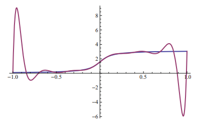
Clearly $u=0$ is a solution, but we can have nonzero solutions corresponding to certain values of the $\mathrm{K}$ known as eigenvalues. The corresponding function $u$ is called an eigenfunction. If $F=0$ then $K=0$ and $u=0$ is the only solution, but if the force is increased it will reach a critical value where the beam will buckle and maybe break. This critical value corresponds to the smallest eigenvalue of (2.25). With $u(t)=\sin (\pi t)$ we find $u^{\prime \prime}(t)=-\pi^{2} u(t)$ and this $u$ is a solution if $K=\pi^{2}$. It can be shown that this is the smallest eigenvalue of (2.25) and solving for $F$ we find $F=\frac{\pi^{2} R}{L^{2}}$.
We can approximate this eigenvalue numerically. Choosing $m \in \mathbb{N}, h:=1 /(m+$
1) and using for the second derivative the approximation
$$
u^{\prime \prime}(j h) \approx \frac{u((j+1) h)-2 u(j h)+u((j-1) h)}{h^{2}}, \quad j=1, \ldots, m,
$$
(this is the same finite difference approximation as in Sect. 2.2) we obtain
$$
\frac{-v_{j-1}+2 v_{j}-v_{j+1}}{h^{2}}=K v_{j}, \quad j=1, \ldots, m, h=\frac{1}{m+1}, \quad v_{0}=v_{m+1}=0
$$
where $v_{j} \approx u(j h)$ for $j=0, \ldots, m+1$. If we define $\lambda:=h^{2} K$ then we obtain the equation
$$
T v=\lambda v, \text { with } v=\left[v_{1}, \ldots, v_{m}\right]^{T}
$$
and
The problem now is to determine the eigenvalues of $T$. Normally we would need a numerical method to determine the eigenvalues of a matrix, but for this simple problem the eigenvalues can be determined exactly. We show in the next subsection that the smallest eigenvalue of $(2.26)$ is given by $\lambda=4 \sin ^{2}(\pi h / 2)$. Since $\lambda=$ $h^{2} K=\frac{h^{2} F L^{2}}{R}$ we can solve for $F$ to obtain
$$
F=\frac{4 \sin ^{2}(\pi h / 2) R}{h^{2} L^{2}}
$$
For small $h$ this is a good approximation to the value $\frac{\pi^{2} R}{L^{2}}$ we computed above.
计算线性代数代考
数学代写|计算线性代数代写Computational Linear Algebra代考|A Two Point Boundary Value Problem
考虑简单的两点边值问题
−在′′(X)=F(X),X∈[0,1],在(0)=0,在(1)=0
在哪里F是一个给定的连续函数[0,1]和在是一个未知函数。此问题也称为一维 (1D) 泊松问题。原则上很容易解决(2.20)确切地。我们只是整合F两次并确定两个积分常数,使均匀边界条件在(0)=在(1)=0 满意。例如,如果F(X)=1然后在(X)=X(X−1)/2是解决方案。
认为F无法准确整合。问题(2.20)然后可以使用有限差分法近似求解。我们需要二阶导数的差分近似。如果G是可微分的函数X然后
G′(X)=林H→0G(X+H2)−G(X−H2)H并将其应用于函数在在X
在′′(X)=林H→0在′(X+H2)−在′(X−H2)H=林H→0在(X+H)−在(X)H−在(X)−在(X−H)HH =林H→0在(X+H)−2在(X)+在(X−H)H2为了定义使用这种差异近似的点,我们选择一个正整数米, 让H:=1/(米+1)为离散化参数,并替换区间[0,1]按网格点Xj:=jH为了j=0,1,…,米+1. 然后我们得到近似值在j到确切的解决方案在(Xj)为了j=1,…,米通过用差分方程代替差分方程
−在j−1+2在j−在j+1H2=F(jH),j=1,…,米,在0=在米+1=0
移动H2右边的因子这可以写成米×米线性系统
矩阵吨称为二阶导数矩阵,在本书中会经常出现。这是我们的第二个三对角矩阵示例,吨=三方(一个一世,d一世,C一世)∈ R米×米, 在这种情况下一个一世=C一世=−1和d一世=2对所有人一世.
数学代写|计算线性代数代写Computational Linear Algebra代考|Diagonal Dominance
我们想证明(2.21)有一个独特的解决方案。注意吨不是严格对角占优。然而,吨根据以下定义,是弱对角占优。
定义2.3(对角优势)矩阵一个=[一个一世j]∈Cn×n如果是弱对角占优
|一个一世一世|≥∑j≠一世|一个一世j|,一世=1,…,n
我们在定理中展示了2.2严格对角占优矩阵是非奇异的。在弱对角占优的情况下,这通常是不正确的。考虑 3 个矩阵
一个1=[110 121 011],一个2=[100 000 001],一个3=[2−10 −12−1 0−12]它们都是弱对角占优,但一个1和一个2是单数的,而一个3是非奇异的。的确,对于一个1第二列是第一列和第三列的总和,一个2有一个零行,并且这(一个3)=4≠0. 因此,对于弱对角占优矩阵的 LU 分解的非奇异性和存在性,我们需要一些额外的条件。这里有一些充分条件。
定理 2.4(弱对角优势)假设一个=三方(一个一世,d一世,C一世)∈ Cn×n是三对角且弱对角占优。如果另外|d1|>|C1|和一个一世≠0为了一世=1,…,n−2, 然后一个有一个独特的大号在因式分解(2.15)。如果另外dn≠0, 然后一个是非奇异的。
证明 证明类似于定理 2.2 的证明。矩阵一个有一个 LU 分解,如果在ķ(2.16) 中的 ‘s 非零ķ=1,…,n−1. 为此,通过归纳表明|在ķ|>|Cķ|为了ķ=1,…,n−1. 假设|在1|=|d1|>|C1|. 认为|在ķ|>|Cķ|对于一些1≤ķ≤n−2. 然后|Cķ|/|在ķ|<1并且由 (2.16) 并且因为一个ķ≠0
|在ķ+1|=|dķ+1−lķCķ|=|dķ+1−一个ķCķ在ķ|≥|dķ+1|−|一个ķ||Cķ||在ķ|>|dķ+1|−|一个ķ|.
这也适用于ķ=n−1如果一个n−1≠0. 由 (2.23) 和弱对角优势|在ķ+1|>|dķ+1|−|一个ķ|≥|Cķ+1|并且通过归纳得出存在LU分解。它是唯一的,因为任何 LU 分解都必须满足 (2.16)。对于非奇异性,我们需要证明在n≠0. 然后由引理2.5, 两个都大号和在是非奇异的,这等价于一个=大号在是非奇异的。如果一个n−1≠0然后由 (2.16)|在n|>|dn|−|一个n−1|≥0通过弱对角优势,而如果一个n−1=0然后再由 (2.23)|在n|≥|dn|>0.
数学代写|计算线性代数代写Computational Linear Algebra代考|The Buckling of a Beam
考虑长度为的水平梁大号位于 0 和大号在X- 平面的轴。我们假设梁固定在X=0和X=大号那是一种力量F应用于(大号,0)朝着原点的方向。这种情况可以用边值问题来建模
R是′′(X)=−F是(X),是(0)=是(大号)=0,
在哪里是(X)是梁的垂直位移X, 和R是由梁的刚度定义的常数。我们可以将问题转化为单位区间[0,1]通过考虑函数在:[0,1]→R由在(吨):=是(吨大号). 自从在′′(吨)= 大号2是′′(吨大号), 问题(2.24)然后变成
在′′(吨)=−ķ在(吨),在(0)=在(1)=0,ķ:=F大号2R.
清楚地在=0是一个解,但我们可以有对应于某些值的非零解ķ称为特征值。对应功能在称为特征函数。如果F=0然后ķ=0和在=0是唯一的解决方案,但如果力增加,它将达到一个临界值,梁将弯曲并可能断裂。该临界值对应于 (2.25) 的最小特征值。和在(吨)=罪(圆周率吨)我们发现在′′(吨)=−圆周率2在(吨)和这个在是一个解决方案,如果ķ=圆周率2. 可以证明这是 (2.25) 的最小特征值,求解F我们发现F=圆周率2R大号2.
我们可以用数值近似这个特征值。选择米∈ñ,H:=1/(米+
1) 并使用二阶导数的近似值
在′′(jH)≈在((j+1)H)−2在(jH)+在((j−1)H)H2,j=1,…,米,
(这与第 2.2 节中的有限差分近似相同)我们得到
−在j−1+2在j−在j+1H2=ķ在j,j=1,…,米,H=1米+1,在0=在米+1=0
在哪里在j≈在(jH)为了j=0,…,米+1. 如果我们定义λ:=H2ķ然后我们得到方程
吨在=λ在, 和 在=[在1,…,在米]吨
现在
的问题是确定吨. 通常我们需要一种数值方法来确定矩阵的特征值,但是对于这个简单的问题,可以准确地确定特征值。我们将在下一小节中展示(2.26)是(谁)给的λ=4罪2(圆周率H/2). 自从λ= H2ķ=H2F大号2R我们可以解决F获得
F=4罪2(圆周率H/2)RH2大号2
对于小H这是一个很好的近似值圆周率2R大号2我们在上面计算。

统计代写请认准statistics-lab™. statistics-lab™为您的留学生涯保驾护航。
金融工程代写
金融工程是使用数学技术来解决金融问题。金融工程使用计算机科学、统计学、经济学和应用数学领域的工具和知识来解决当前的金融问题,以及设计新的和创新的金融产品。
非参数统计代写
非参数统计指的是一种统计方法,其中不假设数据来自于由少数参数决定的规定模型;这种模型的例子包括正态分布模型和线性回归模型。
广义线性模型代考
广义线性模型(GLM)归属统计学领域,是一种应用灵活的线性回归模型。该模型允许因变量的偏差分布有除了正态分布之外的其它分布。
术语 广义线性模型(GLM)通常是指给定连续和/或分类预测因素的连续响应变量的常规线性回归模型。它包括多元线性回归,以及方差分析和方差分析(仅含固定效应)。
有限元方法代写
有限元方法(FEM)是一种流行的方法,用于数值解决工程和数学建模中出现的微分方程。典型的问题领域包括结构分析、传热、流体流动、质量运输和电磁势等传统领域。
有限元是一种通用的数值方法,用于解决两个或三个空间变量的偏微分方程(即一些边界值问题)。为了解决一个问题,有限元将一个大系统细分为更小、更简单的部分,称为有限元。这是通过在空间维度上的特定空间离散化来实现的,它是通过构建对象的网格来实现的:用于求解的数值域,它有有限数量的点。边界值问题的有限元方法表述最终导致一个代数方程组。该方法在域上对未知函数进行逼近。[1] 然后将模拟这些有限元的简单方程组合成一个更大的方程系统,以模拟整个问题。然后,有限元通过变化微积分使相关的误差函数最小化来逼近一个解决方案。
tatistics-lab作为专业的留学生服务机构,多年来已为美国、英国、加拿大、澳洲等留学热门地的学生提供专业的学术服务,包括但不限于Essay代写,Assignment代写,Dissertation代写,Report代写,小组作业代写,Proposal代写,Paper代写,Presentation代写,计算机作业代写,论文修改和润色,网课代做,exam代考等等。写作范围涵盖高中,本科,研究生等海外留学全阶段,辐射金融,经济学,会计学,审计学,管理学等全球99%专业科目。写作团队既有专业英语母语作者,也有海外名校硕博留学生,每位写作老师都拥有过硬的语言能力,专业的学科背景和学术写作经验。我们承诺100%原创,100%专业,100%准时,100%满意。
随机分析代写
随机微积分是数学的一个分支,对随机过程进行操作。它允许为随机过程的积分定义一个关于随机过程的一致的积分理论。这个领域是由日本数学家伊藤清在第二次世界大战期间创建并开始的。
时间序列分析代写
随机过程,是依赖于参数的一组随机变量的全体,参数通常是时间。 随机变量是随机现象的数量表现,其时间序列是一组按照时间发生先后顺序进行排列的数据点序列。通常一组时间序列的时间间隔为一恒定值(如1秒,5分钟,12小时,7天,1年),因此时间序列可以作为离散时间数据进行分析处理。研究时间序列数据的意义在于现实中,往往需要研究某个事物其随时间发展变化的规律。这就需要通过研究该事物过去发展的历史记录,以得到其自身发展的规律。
回归分析代写
多元回归分析渐进(Multiple Regression Analysis Asymptotics)属于计量经济学领域,主要是一种数学上的统计分析方法,可以分析复杂情况下各影响因素的数学关系,在自然科学、社会和经济学等多个领域内应用广泛。
MATLAB代写
MATLAB 是一种用于技术计算的高性能语言。它将计算、可视化和编程集成在一个易于使用的环境中,其中问题和解决方案以熟悉的数学符号表示。典型用途包括:数学和计算算法开发建模、仿真和原型制作数据分析、探索和可视化科学和工程图形应用程序开发,包括图形用户界面构建MATLAB 是一个交互式系统,其基本数据元素是一个不需要维度的数组。这使您可以解决许多技术计算问题,尤其是那些具有矩阵和向量公式的问题,而只需用 C 或 Fortran 等标量非交互式语言编写程序所需的时间的一小部分。MATLAB 名称代表矩阵实验室。MATLAB 最初的编写目的是提供对由 LINPACK 和 EISPACK 项目开发的矩阵软件的轻松访问,这两个项目共同代表了矩阵计算软件的最新技术。MATLAB 经过多年的发展,得到了许多用户的投入。在大学环境中,它是数学、工程和科学入门和高级课程的标准教学工具。在工业领域,MATLAB 是高效研究、开发和分析的首选工具。MATLAB 具有一系列称为工具箱的特定于应用程序的解决方案。对于大多数 MATLAB 用户来说非常重要,工具箱允许您学习和应用专业技术。工具箱是 MATLAB 函数(M 文件)的综合集合,可扩展 MATLAB 环境以解决特定类别的问题。可用工具箱的领域包括信号处理、控制系统、神经网络、模糊逻辑、小波、仿真等。