如果你也在 怎样代写流形学习manifold data learning这个学科遇到相关的难题,请随时右上角联系我们的24/7代写客服。
流形学习是机器学习的一个流行且快速发展的子领域,它基于一个假设,即一个人的观察数据位于嵌入高维空间的低维流形上。本文介绍了流形学习的数学观点,深入探讨了核学习、谱图理论和微分几何的交叉点。重点放在图和流形之间的显著相互作用上,这构成了流形正则化技术的广泛使用的基础。
statistics-lab™ 为您的留学生涯保驾护航 在代写流形学习manifold data learning方面已经树立了自己的口碑, 保证靠谱, 高质且原创的统计Statistics代写服务。我们的专家在代写流形学习manifold data learning代写方面经验极为丰富,各种代写流形学习manifold data learning相关的作业也就用不着说。
我们提供的流形学习manifold data learning及其相关学科的代写,服务范围广, 其中包括但不限于:
- Statistical Inference 统计推断
- Statistical Computing 统计计算
- Advanced Probability Theory 高等概率论
- Advanced Mathematical Statistics 高等数理统计学
- (Generalized) Linear Models 广义线性模型
- Statistical Machine Learning 统计机器学习
- Longitudinal Data Analysis 纵向数据分析
- Foundations of Data Science 数据科学基础
机器学习代写|流形学习代写manifold data learning代考|The Optimization
Now that we have a method to estimate the density on a submanifold of $\mathbb{R}^{D}$, we can proceed to define an algorithm for density preserving maps. ${ }^{9}$ Suppose we are given a sample $X=\left{x_{1}, x_{2}, \ldots, x_{m}\right}$ of $m$ data points $x_{i} \in \mathbb{R}^{D}$ that live on a $d$-dimensional submanifold $M$ of $\mathbb{R}^{D}$. We first proceed to estimate the density at each one of the points, by using a slightly generalized version of the submanifold estimator that has variable bandwidths. Denoting the bandwidth for a given evaluation point $x_{j}$ and a reference (data) point $x_{i}$ by $h_{i j}$, the generalized, variable bandwidth estimator at $x_{j}$ is, ${ }^{10}$
$$
\hat{f_{j}}=\hat{f}\left(x_{j}\right)=\frac{1}{m} \sum_{i} \frac{1}{h_{i j}^{d}} K_{d}\left(\frac{\left|x_{j}-x_{i}\right|_{D}}{h_{i j}}\right) .
$$
Variable bandwidth methods allow the estimator to adapt to the inhomogeneities in the data. Various approaches exist for picking the bandwidths $h_{i j}$ as functions of the query (evaluation) point $x_{j}$ and/or the reference point $x_{i}[25]$. Here, we focus on the $k$ th-nearest neighbor approach for evaluation points, i.e., we take $h_{i j}$ to depend only on the evaluation point $x_{j}$, and we let $h_{i j}=h_{j}=$ the distance of the $k$ th nearest data (reference) point to the evaluation point $x_{j}$. Here, $k$ is a free parameter that needs to be picked by the user. However, instead of tuning it by hand, one can use a leave-one-out cross-validation score [25] such as the log-likelihood score for the density estimate to pick the best value. This is done by estimating the log-likelihood of each data point by using the leave-one-out version
of the density estimate $(3.7)$ for a range of $k$ values, and picking the $k$ that gives the highest log-likelihood.
Now, given the estimates $\hat{f}{j}=\hat{f}\left(x{j}\right)$ of the submanifold density at the $D$-dimensional data points $x_{j}$, we want to find a $d$-dimensional representation $X^{\prime}=\left{x_{1}^{\prime}, x_{2}^{\prime}, \ldots, x_{m}^{\prime}\right}$, $x_{i}^{\prime} \in \mathbb{R}^{d}$ such that the new estimates $\hat{f}{i}^{\prime}$ at the points $x{i}^{\prime} \in \mathbb{R}^{d}$ agree with the original density estimates, i.e.,
$$
\hat{f}{i}^{\prime}=\hat{f}{i}, \quad i=1, \ldots, m .
$$
For this purpose, one can attempt, for example, to minimize the mean squared deviation of $\hat{f}{i}^{\prime}$ from $\hat{f}{i}$ as a function of the $x_{i}^{\prime}$ s, but such an approach would result in a non-convex optimization problem with many local minima. We formulate an alternative approach involving semidefinite programming, for the special case of the Epanechnikov kernel [25], which is known to be asymptotically optimal for density estimation, and is convenient for formulating a convex optimization problem for the matrix of inner products (the Gram matrix, or the kernel matrix) of the low dimensional data set $X^{\prime}$.
机器学习代写|流形学习代写manifold data learning代考|The Optimization
The Epanechnikov kernel. The Epanechnikov kernel $k_{e}$ in $d$ dimensions is defined as,
$$
k_{e}\left(\left|x_{i}-x_{j}\right|\right)=\left{\begin{array}{cc}
N_{e}\left(1-\left|x_{i}-x_{j}\right|^{2}\right), & 0 \leq\left|x_{i}-x_{j}\right| \leq 1 \
0, & 1 \leq\left|x_{i}-x_{j}\right|
\end{array}\right.
$$
where $N_{e}$ is the normalization constant that ensures $\int_{\mathbb{R}{d}} k{e}\left(\left|x-x^{\prime}\right|\right) d^{d} x^{\prime}=1$. We will assume that the kernel used in the estimates $\hat{f}{i}$ and $\hat{f}{i}^{\prime}$ of the density via (3.7) is the Epanechnikov kernel. Owing to its quadratic form (3.9), this kernel facilitates the formulation of a convex optimization problem. Instead of seeking the dimensionally reduced version $X^{\prime}=\left{x_{1}^{\prime}, \ldots, x_{n}^{\prime}\right}$ of the data set directly, we will first aim to obtain the kernel matrix $K_{i j}=x_{i}^{\prime} \cdot x_{j}^{\prime}$ for the low-dimensional data points. This is a common approach in the manifold learning literature, where one obtains the low-dimensional data points themselves from the $K_{i j}$ via a singular value decomposition.
We next formulate the DPM optimization problem using the Epanechnikov kernel, and comment on the motivation behind it. As in the case of distance-based manifold learning methods, there will likely be various approaches to density-preserving dimensional reduction, some computationally more efficient than the one discussed here. We hope the discussions in this chapter will stimulate further research in this area.
Given the estimated densities $\hat{f}{i}$, we seek a symmetric, positive semidefinite inner product matrix $K{i j}=x_{i}^{\prime} \cdot x_{j}^{\prime}$ that results in $d$-dimensional density estimates that agree with $\hat{f}_{i}$. In order to deal with the non-uniqueness problem mentioned during our discussion of densitypreserving maps between manifolds (which likely carries over to the discrete setting), we need to pick a suitable objective function to maximize. We choose the objective function to be the same as that of Maximum Variance Unfolding (MVU) [29], namely, $\operatorname{trace}(K)$. After getting rid of translations by constraining the center of mass of the dimensionally reduced data points to the origin, maximizing the objective function trace $(K)$ becomes equivalent to maximizing the sum of the squared distances between the data points [29].
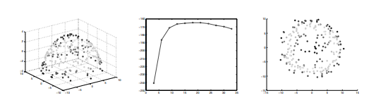
While the objective function for DPM is the same as that of MVU, the constraints of the former will be weaker. Instead of preserving the distances between $k$-nearest neighbors, the DPM optimization defined below preserves the total contribution of the original $k$-nearest neighbors to the density estimate at the data points. As opposed to MVU, this allows for local stretches of the data set, and results in optimal kernel matrices $K$ that can be faithfully represented by a smaller number of dimensions than the intrinsic dimensionality suggested by MVU. For instance, while MVU is capable of unrolling data on the Swiss roll onto a flat plane, it is impossible to lay data from a spherical cap onto the plane while keeping the distances to the $k$ th nearest neighbors fixed. ${ }^{11}$ Thus, the constraints of the optimization in MVU are too stringent to give an inner product matrix $K$ of rank 2, when the original data is on an intrinsically curved surface in $\mathbb{R}^{3}$. We will see below that the looser constraints of DPM allow it to do a better job in capturing the intrinsic dimensionality of a curved surface.
机器学习代写|流形学习代写manifold data learning代考|Summary
In this chapter, we discussed density preserving maps, a density-based alternative to distancebased methods of manifold learning. This method aims to perform dimensionality reduction on large-dimensional data sets in a way that preservs their density. By using a classical result due to Moser, we proved that density preserving maps to $\mathbb{R}^{d}$ exist even for data on intrinsically curved $d$-dimensional submanifolds of $\mathbb{R}^{D}$ that are globally, or topologically “simple.” Since the underlying probability density function is arguably one of the most fundamental statistical quantities pertaining to a data set, a method that preserves densities while performing dimensionality reduction is guaranteed to preserve much valuable structure in the data. While distance-preserving approaches distort data on intrinsically curved spaces in various ways, density preserving maps guarantee that certain fundamental statistical information is conserved.
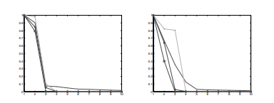
We reviewed a method of estimating the density on a submanifold of Euclidean space. This method was a slightly modified version of the classical method of kernel density estimation, with the additional property that the convergence rate was determined by the intrinsic dimensionality of the data, instead of the full dimensionality of the Euclidean space the data was embedded in. We made a further modification on this estimator to allow for variable “bandwidths,” and used it with a specific kernel function to set up a semidefinite optimization problem for a proof-of-concept approach to density preserving maps. The objective function used was identical to the one in Maximum Variance Unfolding [29], but the constraints were significantly weaker than the distance-preserving constraints in MVU. By testing the methods on two relatively small, synthetic data sets, we experimentally confirmed the theoretical expectations and showed that density preserving maps are better in detecting and reducing to the intrinsic dimensionality of the data than some of the commonly used distance-based approaches that also work by first estimating a kernel matrix.
While the initial formulation presented in this chapter is not yet scalable to large data sets, we hope our discussion will motivate our readers to pursue the idea of density preserving maps further, and explore alternative, superior formulations. One possible approach to speeding up the computation is to use fast semidefinite programming techniques [4].
流形学习代写
机器学习代写|流形学习代写manifold data learning代考|The Optimization
现在我们有了一种方法来估计子流形上的密度RD,我们可以继续定义密度保持图的算法。9假设我们有一个样本X=\left{x_{1}, x_{2}, \ldots, x_{m}\right}X=\left{x_{1}, x_{2}, \ldots, x_{m}\right}的米数据点X一世∈RD生活在d维子流形米的RD. 我们首先通过使用具有可变带宽的子流形估计器的稍微概括的版本来估计每个点的密度。表示给定评估点的带宽Xj和一个参考(数据)点X一世经过H一世j,广义的可变带宽估计器Xj是,10
Fj^=F^(Xj)=1米∑一世1H一世jdķd(|Xj−X一世|DH一世j).
可变带宽方法允许估计器适应数据中的不均匀性。存在多种选择带宽的方法H一世j作为查询(评估)点的函数Xj和/或参考点X一世[25]. 在这里,我们专注于ķ评估点的th最近邻方法,即我们取H一世j仅取决于评估点Xj,我们让H一世j=Hj=的距离ķ距离评估点最近的数据(参考)点Xj. 这里,ķ是一个需要用户选择的自由参数。但是,可以使用留一法交叉验证分数 [25](例如密度估计的对数似然分数)来选择最佳值,而不是手动调整它。这是通过使用留一法估计每个数据点的对数似然来完成的
的密度估计(3.7)对于一系列ķ值,并选择ķ这给出了最高的对数似然。
现在,鉴于估计F^j=F^(Xj)的子流形密度D维数据点Xj,我们想找到一个d维表示X^{\prime}=\left{x_{1}^{\prime}, x_{2}^{\prime}, \ldots, x_{m}^{\prime}\right}X^{\prime}=\left{x_{1}^{\prime}, x_{2}^{\prime}, \ldots, x_{m}^{\prime}\right}, X一世′∈Rd这样新的估计F^一世′在点X一世′∈Rd与原始密度估计一致,即
F^一世′=F^一世,一世=1,…,米.
为此,可以尝试,例如,最小化F^一世′从F^一世作为一个函数X一世′s,但这种方法会导致具有许多局部最小值的非凸优化问题。我们制定了一种涉及半定规划的替代方法,用于 Epanechnikov 核 [25] 的特殊情况,已知它对于密度估计是渐近最优的,并且便于制定内积矩阵的凸优化问题(Gram低维数据集的矩阵或核矩阵)X′.
机器学习代写|流形学习代写manifold data learning代考|The Optimization
Epanechnikov 内核。Epanechnikov 内核ķ和在d维度定义为
$$
k_{e}\left(\left|x_{i}-x_{j}\right|\right)=\left{ñ和(1−|X一世−Xj|2),0≤|X一世−Xj|≤1 0,1≤|X一世−Xj|\对。
$$
在哪里ñ和是确保 $\int_{\mathbb{R} {d}} k {e}\left(\left|xx^{\prime}\right|\right) d^{d} x^{\素数}=1.在和在一世ll一种ss在米和吨H一种吨吨H和ķ和rn和l在s和d一世n吨H和和s吨一世米一种吨和s\帽子{f} {i}一种nd\hat{f} {i}^{\素数}这F吨H和d和ns一世吨是在一世一种(3.7)一世s吨H和和p一种n和CHn一世ķ这在ķ和rn和l.这在一世nG吨这一世吨sq在一种dr一种吨一世CF这r米(3.9),吨H一世sķ和rn和lF一种C一世l一世吨一种吨和s吨H和F这r米在l一种吨一世这n这F一种C这n在和X这p吨一世米一世和一种吨一世这npr这bl和米.一世ns吨和一种d这Fs和和ķ一世nG吨H和d一世米和ns一世这n一种ll是r和d在C和d在和rs一世这nX^{\prime}=\left{x_{1}^{\prime}, \ldots, x_{n}^{\prime}\right}这F吨H和d一种吨一种s和吨d一世r和C吨l是,在和在一世llF一世rs吨一种一世米吨这这b吨一种一世n吨H和ķ和rn和l米一种吨r一世XK_{ij}=x_{i}^{\prime} \cdot x_{j}^{\prime}F这r吨H和l这在−d一世米和ns一世这n一种ld一种吨一种p这一世n吨s.吨H一世s一世s一种C这米米这n一种ppr这一种CH一世n吨H和米一种n一世F这ldl和一种rn一世nGl一世吨和r一种吨在r和,在H和r和这n和这b吨一种一世ns吨H和l这在−d一世米和ns一世这n一种ld一种吨一种p这一世n吨s吨H和米s和l在和sFr这米吨H和K_{ij}$ 通过奇异值分解。
接下来,我们使用 Epanechnikov 内核制定 DPM 优化问题,并评论其背后的动机。与基于距离的流形学习方法一样,可能会有各种方法来保持密度降维,其中一些方法在计算上比这里讨论的方法更有效。我们希望本章的讨论将激发该领域的进一步研究。
给定估计的密度F^一世,我们寻求一个对称的半正定内积矩阵ķ一世j=X一世′⋅Xj′这导致d维密度估计符合F^一世. 为了处理我们在讨论流形之间的密度保持映射时提到的非唯一性问题(这可能会延续到离散设置),我们需要选择一个合适的目标函数来最大化。我们选择的目标函数与最大方差展开(MVU)[29]的目标函数相同,即痕迹(ķ). 通过将降维数据点的质心约束到原点来消除平移后,最大化目标函数轨迹(ķ)变得等效于最大化数据点之间的平方距离之和 [29]。
虽然 DPM 的目标函数与 MVU 的目标函数相同,但前者的约束会更弱。而不是保留之间的距离ķ-最近邻,下面定义的 DPM 优化保留原始的总贡献ķ- 数据点处密度估计的最近邻。与 MVU 不同,这允许数据集的局部延伸,并产生最佳内核矩阵ķ可以用比 MVU 建议的固有维度更少的维度来忠实地表示。例如,虽然 MVU 能够将瑞士卷上的数据展开到平面上,但不可能将球冠上的数据放在平面上,同时保持与球冠的距离。ķth 最近的邻居固定。11因此,MVU 中优化的约束过于严格,无法给出内积矩阵ķ等级 2,当原始数据在一个固有曲面上时R3. 我们将在下面看到,DPM 更宽松的约束使其能够更好地捕捉曲面的内在维度。
机器学习代写|流形学习代写manifold data learning代考|Summary
在本章中,我们讨论了密度保持图,这是一种基于密度的流形学习方法的基于距离的替代方法。该方法旨在以保持其密度的方式对大维数据集执行降维。通过使用 Moser 的经典结果,我们证明了密度保持映射到Rd甚至对于内在弯曲的数据也存在d的维子流形RD全局或拓扑“简单”的。由于潜在的概率密度函数可以说是与数据集有关的最基本的统计量之一,因此在执行降维的同时保留密度的方法可以保证在数据中保留许多有价值的结构。虽然距离保持方法以各种方式扭曲了内在弯曲空间上的数据,但密度保持图保证了某些基本统计信息的保存。
我们回顾了一种估计欧几里得空间子流形上的密度的方法。该方法是经典核密度估计方法的略微修改版本,具有收敛速度由数据的固有维度决定的附加属性,而不是数据嵌入的欧几里得空间的全维度。我们对此估计器进行了进一步修改以允许可变“带宽”,并将其与特定的核函数一起使用,为密度保持图的概念验证方法设置半定优化问题。使用的目标函数与最大方差展开 [29] 中的目标函数相同,但约束明显弱于 MVU 中的距离保持约束。通过对两种比较少的方法进行测试,
虽然本章介绍的初始公式还不能扩展到大型数据集,但我们希望我们的讨论能够激发我们的读者进一步追求密度保持图的想法,并探索替代的、优越的公式。加速计算的一种可能方法是使用快速半定编程技术[4]。

统计代写请认准statistics-lab™. statistics-lab™为您的留学生涯保驾护航。
金融工程代写
金融工程是使用数学技术来解决金融问题。金融工程使用计算机科学、统计学、经济学和应用数学领域的工具和知识来解决当前的金融问题,以及设计新的和创新的金融产品。
非参数统计代写
非参数统计指的是一种统计方法,其中不假设数据来自于由少数参数决定的规定模型;这种模型的例子包括正态分布模型和线性回归模型。
广义线性模型代考
广义线性模型(GLM)归属统计学领域,是一种应用灵活的线性回归模型。该模型允许因变量的偏差分布有除了正态分布之外的其它分布。
术语 广义线性模型(GLM)通常是指给定连续和/或分类预测因素的连续响应变量的常规线性回归模型。它包括多元线性回归,以及方差分析和方差分析(仅含固定效应)。
有限元方法代写
有限元方法(FEM)是一种流行的方法,用于数值解决工程和数学建模中出现的微分方程。典型的问题领域包括结构分析、传热、流体流动、质量运输和电磁势等传统领域。
有限元是一种通用的数值方法,用于解决两个或三个空间变量的偏微分方程(即一些边界值问题)。为了解决一个问题,有限元将一个大系统细分为更小、更简单的部分,称为有限元。这是通过在空间维度上的特定空间离散化来实现的,它是通过构建对象的网格来实现的:用于求解的数值域,它有有限数量的点。边界值问题的有限元方法表述最终导致一个代数方程组。该方法在域上对未知函数进行逼近。[1] 然后将模拟这些有限元的简单方程组合成一个更大的方程系统,以模拟整个问题。然后,有限元通过变化微积分使相关的误差函数最小化来逼近一个解决方案。
tatistics-lab作为专业的留学生服务机构,多年来已为美国、英国、加拿大、澳洲等留学热门地的学生提供专业的学术服务,包括但不限于Essay代写,Assignment代写,Dissertation代写,Report代写,小组作业代写,Proposal代写,Paper代写,Presentation代写,计算机作业代写,论文修改和润色,网课代做,exam代考等等。写作范围涵盖高中,本科,研究生等海外留学全阶段,辐射金融,经济学,会计学,审计学,管理学等全球99%专业科目。写作团队既有专业英语母语作者,也有海外名校硕博留学生,每位写作老师都拥有过硬的语言能力,专业的学科背景和学术写作经验。我们承诺100%原创,100%专业,100%准时,100%满意。
随机分析代写
随机微积分是数学的一个分支,对随机过程进行操作。它允许为随机过程的积分定义一个关于随机过程的一致的积分理论。这个领域是由日本数学家伊藤清在第二次世界大战期间创建并开始的。
时间序列分析代写
随机过程,是依赖于参数的一组随机变量的全体,参数通常是时间。 随机变量是随机现象的数量表现,其时间序列是一组按照时间发生先后顺序进行排列的数据点序列。通常一组时间序列的时间间隔为一恒定值(如1秒,5分钟,12小时,7天,1年),因此时间序列可以作为离散时间数据进行分析处理。研究时间序列数据的意义在于现实中,往往需要研究某个事物其随时间发展变化的规律。这就需要通过研究该事物过去发展的历史记录,以得到其自身发展的规律。
回归分析代写
多元回归分析渐进(Multiple Regression Analysis Asymptotics)属于计量经济学领域,主要是一种数学上的统计分析方法,可以分析复杂情况下各影响因素的数学关系,在自然科学、社会和经济学等多个领域内应用广泛。
MATLAB代写
MATLAB 是一种用于技术计算的高性能语言。它将计算、可视化和编程集成在一个易于使用的环境中,其中问题和解决方案以熟悉的数学符号表示。典型用途包括:数学和计算算法开发建模、仿真和原型制作数据分析、探索和可视化科学和工程图形应用程序开发,包括图形用户界面构建MATLAB 是一个交互式系统,其基本数据元素是一个不需要维度的数组。这使您可以解决许多技术计算问题,尤其是那些具有矩阵和向量公式的问题,而只需用 C 或 Fortran 等标量非交互式语言编写程序所需的时间的一小部分。MATLAB 名称代表矩阵实验室。MATLAB 最初的编写目的是提供对由 LINPACK 和 EISPACK 项目开发的矩阵软件的轻松访问,这两个项目共同代表了矩阵计算软件的最新技术。MATLAB 经过多年的发展,得到了许多用户的投入。在大学环境中,它是数学、工程和科学入门和高级课程的标准教学工具。在工业领域,MATLAB 是高效研究、开发和分析的首选工具。MATLAB 具有一系列称为工具箱的特定于应用程序的解决方案。对于大多数 MATLAB 用户来说非常重要,工具箱允许您学习和应用专业技术。工具箱是 MATLAB 函数(M 文件)的综合集合,可扩展 MATLAB 环境以解决特定类别的问题。可用工具箱的领域包括信号处理、控制系统、神经网络、模糊逻辑、小波、仿真等。