如果你也在 怎样代写广义相对论General relativity这个学科遇到相关的难题,请随时右上角联系我们的24/7代写客服。
广义相对论是阿尔伯特-爱因斯坦在1907至1915年间提出的引力理论。广义相对论说,观察到的质量之间的引力效应是由它们对时空的扭曲造成的。
statistics-lab™ 为您的留学生涯保驾护航 在代写广义相对论General relativity方面已经树立了自己的口碑, 保证靠谱, 高质且原创的统计Statistics代写服务。我们的专家在代写广义相对论General relativity代写方面经验极为丰富,各种代写广义相对论General relativity相关的作业也就用不着说。
我们提供的广义相对论General relativity及其相关学科的代写,服务范围广, 其中包括但不限于:
- Statistical Inference 统计推断
- Statistical Computing 统计计算
- Advanced Probability Theory 高等概率论
- Advanced Mathematical Statistics 高等数理统计学
- (Generalized) Linear Models 广义线性模型
- Statistical Machine Learning 统计机器学习
- Longitudinal Data Analysis 纵向数据分析
- Foundations of Data Science 数据科学基础
物理代写|广义相对论代写General relativity代考|Geodesics as Self-parallel Curves
We now know how to displace a vector to a nearby point so that it remains parallel to itself in the general sense defined in the preceding two sections. We may use this to define and study the idea of a generalized straight line or geodesic. Our definition of a geodesic stems naturally from classical Euclidean geometry and intuition. Suppose we have a curve $C$ specified by giving the coordinates as functions of some scalar parameter $p$ which labels points on $C$,
Curve $C: x^{\mu}=x^{\mu}(p)$
We call $C$ a geodesic if it is everywhere parallel to itself; this means that if we parallel displace a tangent vector along $C$ then it remains a tangent vector.
This definition leads to a differential equation for the geodesic. Call the tangent vector $t^{\alpha}(p)$ at $p$. We parallel displace it along the curve to a nearby point labeled $p^{\prime}$ at a coordinate distance $\mathrm{d} x^{\alpha}$ to obtain
$$
t^{* \alpha}\left(p^{\prime}\right)=t^{\alpha}(p)-\Gamma_{\beta \gamma}^{\alpha} \mathrm{d} x^{\beta} t^{\gamma}(p)
$$
The actual tangent at $p^{\prime}$ may be obtained from that at $p$ by a Taylor Series expansion
$$
t^{\alpha}\left(p^{\prime}\right)=t^{\alpha}(p)+\frac{\mathrm{d} t^{\alpha}}{\mathrm{d} p} \mathrm{~d} p
$$
By our above definition of a geodesic the parallel displaced tangent vector in (5.23) is to be equal to the actual tangent vector in $(5.24)$, so that
$$
\frac{\mathrm{d} t^{\alpha}}{\mathrm{d} p} \mathrm{~d} p=-\Gamma_{\beta \gamma}^{\alpha} \mathrm{d} x^{\beta} t^{\gamma}
$$
We may choose the curve parameter $p$ to be the curve length, that is $\mathrm{d} p=\mathrm{d} s$, and use the normalized position derivative as an obvious tangent vector, normalized to unity,
$$
t^{\beta}=\frac{\mathrm{d} x^{\beta}}{\mathrm{d} s}
$$
Substituting this into (5.25) we obtain a differential equation for the geodesic
$$
\frac{\mathrm{d}^{2} x^{\alpha}}{\mathrm{d} s^{2}}+\Gamma_{\beta \gamma}^{\alpha} \frac{\mathrm{d} x^{\beta}}{\mathrm{d} s} \frac{\mathrm{d} x^{\gamma}}{\mathrm{d} s}=0
$$
物理代写|广义相对论代写General relativity代考|Geodesics as Extremum Curves
The self-parallel definition of a geodesic is one of several equivalent ones. In Euclidean geometry a straight line is the shortest distance between two given points. This property can be generalized to give the following definition of a geodesic: let the curve $C$ have length $s$ between two fixed points; then $C$ is a geodesic if the length $s$ is an extremum, that is it is either the shortest or longest among all nearby curves. We will show that this definition leads to the differential equation (5.28) and is equivalent to the self-parallel definition. The extremum calculation is a problem in the calculus of variations, well-known in classical mechanics. If the reader is not familiar with such problems and the Euler-Lagrange method of solution he should first consult Appendix $2 .$
As before the curve $C$ is denoted by
$$
\text { Curve } C: x^{\mu}=x^{\mu}(p) \text {. }
$$
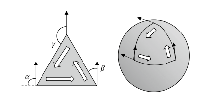
Here $p$ is an invariant parameter, which may be the arc length of the curve but need not be. This is shown schematically in Fig. $5.5$.
The line element along the curve and the arc length $s$ can be written as
$$
\begin{gathered}
\mathrm{d} s^{2}=g_{\alpha \beta} \mathrm{d} x^{\alpha} \mathrm{d} x^{\beta}=g_{\alpha \beta} \dot{x}^{\alpha} \dot{x}^{\beta} \mathrm{d} p^{2} \equiv T\left(x^{\lambda}, \dot{x}^{\kappa}\right) \mathrm{d} p^{2}, \quad \dot{x}^{\kappa} \equiv \frac{\mathrm{d} x^{\kappa}}{\mathrm{d} p} \
s=\int_{i}^{f} \sqrt{g_{\alpha \beta} \dot{x}^{\alpha} \dot{x}^{\beta}} \mathrm{d} p=\int_{i}^{f} \sqrt{T\left(x^{\lambda}, \dot{x}^{\kappa}\right)} \mathrm{d} p
\end{gathered}
$$
where we have assumed the line element $\mathrm{d} s^{2}$ is positive. Finding the extremum of this arc length integral is a standard problem in the calculus of variations and solvable by the Euler-Lagrange method. Indeed it is the analog of a classical mechanics problem with a Lagrangian
$$
L=\sqrt{T\left(x^{\lambda}, \dot{x}^{x}\right)}, \quad T\left(x^{\lambda}, \dot{x}^{\kappa}\right) \equiv g_{\alpha \beta} \dot{x}^{\alpha} \dot{x}^{\beta} .
$$
物理代写|广义相对论代写General relativity代考|Affine Connections, Abstract View
Let us see how we may motivate and interpret the coefficients of affine connection using the abstract view introduced in Sect. 4.3. Recall that a vector may be expanded in a coordinate basis, that is vectors aligned along the coordinate axes, according to
$$
\vec{V}=V^{j} \vec{e}{j}, \quad \vec{e}{j}=\text { coordinate basis. }
$$
If we think of moving the vector to a nearby point it will change due to a change in its components and also a change in the basis vectors,
$$
\mathrm{d} \vec{V}=\vec{e}{i} \mathrm{~d} V^{i}+V^{j} \mathrm{~d} \vec{e}{j}
$$
As we discussed previously the vector spaces associated with different points in a Riemann space are ab initio independent. As such it is necessary to postulate a way to relate them. This leads to the idea of vector transplantation and the specific version of transplantation called parallel displacement that we discussed in Sects. $5.1$ and 5.3. We can think of this in the present abstract view as giving an effective change in the coordinate basis, which we assume is a bilinear expression in the basis vectors and the coordinate displacement; it is a rather compelling assumption. That is we postulate
$$
\mathrm{d} \vec{e}{j}=\Gamma{k j}^{i}\left(\vec{e}_{i} \mathrm{~d} x^{k}\right) .
$$
广义相对论代考
物理代写|广义相对论代写General relativity代考|Geodesics as Self-parallel Curves
我们现在知道如何将向量移动到附近的点,以使其保持与前两节定义的一般意义上的自身平行。我们可以用它来定义和研究广义直线或测地线的概念。我们对测地线的定义自然源于经典的欧几里得几何和直觉。假设我们有一条曲线C通过将坐标指定为某个标量参数的函数p哪些标签指向C,
曲线C:Xμ=Xμ(p)
我们称之为C如果它处处平行于自身,则为测地线;这意味着如果我们沿平行位移一个切向量C那么它仍然是一个切向量。
该定义导致测地线的微分方程。调用切向量吨一个(p)在p. 我们将它沿曲线平行移动到附近标记为的点p′在坐标距离dX一个获得
吨∗一个(p′)=吨一个(p)−ΓbC一个dXb吨C(p)
实际切线在p′可以从中获得p由泰勒级数展开
吨一个(p′)=吨一个(p)+d吨一个dp dp
根据我们上面对测地线的定义,(5.23) 中的平行位移切向量等于(5.24), 以便
d吨一个dp dp=−ΓbC一个dXb吨C
我们可以选择曲线参数p为曲线长度,即dp=ds,并使用归一化的位置导数作为明显的切向量,归一化为单位,
吨b=dXbds
将其代入 (5.25) 我们得到测地线的微分方程
d2X一个ds2+ΓbC一个dXbdsdXCds=0
物理代写|广义相对论代写General relativity代考|Geodesics as Extremum Curves
测地线的自平行定义是几个等效定义之一。在欧几里得几何中,直线是两个给定点之间的最短距离。这个性质可以概括为给出测地线的以下定义:让曲线C有长度s两个固定点之间;然后C如果长度是测地线s是一个极值,即它是所有附近曲线中最短或最长的。我们将证明这个定义导致了微分方程(5.28)并且等价于自平行定义。极值计算是变分法中的一个问题,在经典力学中是众所周知的。如果读者不熟悉此类问题和欧拉-拉格朗日解法,应先查阅附录2.
和之前的曲线一样C表示为
曲线 C:Xμ=Xμ(p).
这里p是一个不变的参数,它可以是曲线的弧长,但不一定是。这在图 1 中示意性地显示。5.5.
沿曲线的线元素和弧长s可以写成
ds2=G一个bdX一个dXb=G一个bX˙一个X˙bdp2≡吨(Xλ,X˙ķ)dp2,X˙ķ≡dXķdp s=∫一世FG一个bX˙一个X˙bdp=∫一世F吨(Xλ,X˙ķ)dp
我们假设线元素ds2是积极的。求弧长积分的极值是变分法中的一个标准问题,可以通过欧拉-拉格朗日方法求解。实际上,它是具有拉格朗日算子的经典力学问题的类比
大号=吨(Xλ,X˙X),吨(Xλ,X˙ķ)≡G一个bX˙一个X˙b.
物理代写|广义相对论代写General relativity代考|Affine Connections, Abstract View
让我们看看如何使用 Sect 中介绍的抽象视图来激发和解释仿射连接系数。4.3. 回想一下,向量可以在坐标基础上展开,即沿着坐标轴对齐的向量,根据
在→=在j和→j,和→j= 坐标基础。
如果我们考虑将向量移动到附近的点,它将由于其分量的变化以及基向量的变化而发生变化,
d在→=和→一世 d在一世+在j d和→j
正如我们之前所讨论的,与黎曼空间中的不同点相关的向量空间是从头算独立的。因此,有必要假设一种将它们联系起来的方法。这导致了向量移植的想法以及我们在 Sects 中讨论的称为平行位移的特定移植版本。5.1和 5.3。在目前的抽象视图中,我们可以认为这是对坐标基础的有效改变,我们假设它是基础向量和坐标位移的双线性表达式;这是一个相当令人信服的假设。那就是我们假设
d和→j=Γķj一世(和→一世 dXķ).

统计代写请认准statistics-lab™. statistics-lab™为您的留学生涯保驾护航。
金融工程代写
金融工程是使用数学技术来解决金融问题。金融工程使用计算机科学、统计学、经济学和应用数学领域的工具和知识来解决当前的金融问题,以及设计新的和创新的金融产品。
非参数统计代写
非参数统计指的是一种统计方法,其中不假设数据来自于由少数参数决定的规定模型;这种模型的例子包括正态分布模型和线性回归模型。
广义线性模型代考
广义线性模型(GLM)归属统计学领域,是一种应用灵活的线性回归模型。该模型允许因变量的偏差分布有除了正态分布之外的其它分布。
术语 广义线性模型(GLM)通常是指给定连续和/或分类预测因素的连续响应变量的常规线性回归模型。它包括多元线性回归,以及方差分析和方差分析(仅含固定效应)。
有限元方法代写
有限元方法(FEM)是一种流行的方法,用于数值解决工程和数学建模中出现的微分方程。典型的问题领域包括结构分析、传热、流体流动、质量运输和电磁势等传统领域。
有限元是一种通用的数值方法,用于解决两个或三个空间变量的偏微分方程(即一些边界值问题)。为了解决一个问题,有限元将一个大系统细分为更小、更简单的部分,称为有限元。这是通过在空间维度上的特定空间离散化来实现的,它是通过构建对象的网格来实现的:用于求解的数值域,它有有限数量的点。边界值问题的有限元方法表述最终导致一个代数方程组。该方法在域上对未知函数进行逼近。[1] 然后将模拟这些有限元的简单方程组合成一个更大的方程系统,以模拟整个问题。然后,有限元通过变化微积分使相关的误差函数最小化来逼近一个解决方案。
tatistics-lab作为专业的留学生服务机构,多年来已为美国、英国、加拿大、澳洲等留学热门地的学生提供专业的学术服务,包括但不限于Essay代写,Assignment代写,Dissertation代写,Report代写,小组作业代写,Proposal代写,Paper代写,Presentation代写,计算机作业代写,论文修改和润色,网课代做,exam代考等等。写作范围涵盖高中,本科,研究生等海外留学全阶段,辐射金融,经济学,会计学,审计学,管理学等全球99%专业科目。写作团队既有专业英语母语作者,也有海外名校硕博留学生,每位写作老师都拥有过硬的语言能力,专业的学科背景和学术写作经验。我们承诺100%原创,100%专业,100%准时,100%满意。
随机分析代写
随机微积分是数学的一个分支,对随机过程进行操作。它允许为随机过程的积分定义一个关于随机过程的一致的积分理论。这个领域是由日本数学家伊藤清在第二次世界大战期间创建并开始的。
时间序列分析代写
随机过程,是依赖于参数的一组随机变量的全体,参数通常是时间。 随机变量是随机现象的数量表现,其时间序列是一组按照时间发生先后顺序进行排列的数据点序列。通常一组时间序列的时间间隔为一恒定值(如1秒,5分钟,12小时,7天,1年),因此时间序列可以作为离散时间数据进行分析处理。研究时间序列数据的意义在于现实中,往往需要研究某个事物其随时间发展变化的规律。这就需要通过研究该事物过去发展的历史记录,以得到其自身发展的规律。
回归分析代写
多元回归分析渐进(Multiple Regression Analysis Asymptotics)属于计量经济学领域,主要是一种数学上的统计分析方法,可以分析复杂情况下各影响因素的数学关系,在自然科学、社会和经济学等多个领域内应用广泛。
MATLAB代写
MATLAB 是一种用于技术计算的高性能语言。它将计算、可视化和编程集成在一个易于使用的环境中,其中问题和解决方案以熟悉的数学符号表示。典型用途包括:数学和计算算法开发建模、仿真和原型制作数据分析、探索和可视化科学和工程图形应用程序开发,包括图形用户界面构建MATLAB 是一个交互式系统,其基本数据元素是一个不需要维度的数组。这使您可以解决许多技术计算问题,尤其是那些具有矩阵和向量公式的问题,而只需用 C 或 Fortran 等标量非交互式语言编写程序所需的时间的一小部分。MATLAB 名称代表矩阵实验室。MATLAB 最初的编写目的是提供对由 LINPACK 和 EISPACK 项目开发的矩阵软件的轻松访问,这两个项目共同代表了矩阵计算软件的最新技术。MATLAB 经过多年的发展,得到了许多用户的投入。在大学环境中,它是数学、工程和科学入门和高级课程的标准教学工具。在工业领域,MATLAB 是高效研究、开发和分析的首选工具。MATLAB 具有一系列称为工具箱的特定于应用程序的解决方案。对于大多数 MATLAB 用户来说非常重要,工具箱允许您学习和应用专业技术。工具箱是 MATLAB 函数(M 文件)的综合集合,可扩展 MATLAB 环境以解决特定类别的问题。可用工具箱的领域包括信号处理、控制系统、神经网络、模糊逻辑、小波、仿真等。