如果你也在 怎样代写广义相对论General relativity这个学科遇到相关的难题，请随时右上角联系我们的24/7代写客服。

广义相对论是阿尔伯特-爱因斯坦在1907至1915年间提出的引力理论。广义相对论说，观察到的质量之间的引力效应是由它们对时空的扭曲造成的。

statistics-lab™ 为您的留学生涯保驾护航 在代写广义相对论General relativity方面已经树立了自己的口碑, 保证靠谱, 高质且原创的统计Statistics代写服务。我们的专家在代写广义相对论General relativity代写方面经验极为丰富，各种代写广义相对论General relativity相关的作业也就用不着说。

我们提供的广义相对论General relativity及其相关学科的代写，服务范围广, 其中包括但不限于:

• Statistical Inference 统计推断
• Statistical Computing 统计计算
• Advanced Probability Theory 高等概率论
• Advanced Mathematical Statistics 高等数理统计学
• (Generalized) Linear Models 广义线性模型
• Statistical Machine Learning 统计机器学习
• Longitudinal Data Analysis 纵向数据分析
• Foundations of Data Science 数据科学基础

物理代写|广义相对论代写General relativity代考|A Special Coordinate System

Recall that in Chap. 4 we stated the Signature Theorem, that at any point $P$ there exists a special coordinate system in which the metric is diagonal and has diagonal elements equal to 1 or $-1$ or 0 . The special system may be reached by a linear transformation. This form of the metric is called the Cayley-Sylvester canonical form. We proved the theorem for the case of two dimensions in Appendix 4.1 (Perlis 1952).

In this chapter we obtained another special coordinate system, the geodesic system, in which the affine connections vanish at any given point $P$. If the connections are zero, then from the definition of the Christoffel connections (5.19) this clearly means that the first derivatives of the metric must also be zero. We can in fact combine these transformations and for any given point $P$ find a coordinate system in which the metric has the Cayley-Sylvester canonical form and also has vanishing first derivatives and thus vanishing connections. To do this we merely apply the two transformations together with the point $P$ taken to be the origin,
$$
\bar{x}^{j}=L_{k}^{j} x^{k}+\frac{1}{2} A_{j l}^{i}\left(L_{n}^{j} x^{n}\right)\left(L_{m}^{l} x^{m}\right) \text {. }
$$
The $L$ array makes the transformation to the system in which the metric has the Cayley-Sylvester canonical form, and the $A$ array specifies the transformation to the geodesic system. The coordinate system thus obtained is very special: the axes are orthogonal, the metric is Lorentz, and the connections vanish, so physics is locally much like that of special relativity, but of course only in a vanishingly small region near $P$.

物理代写|广义相对论代写General relativity代考|The Extremum Problem

For completeness we briefly review one of the most important problems in the calculus of variations, one which is familiar to most physicists from the Lagrangian formulation of classical mechanics (Goldstein 1980). The Lagrangian is assumed to be a given function of the coordinates and generalized velocities, $L\left(x^{\lambda}, \dot{x}^{\alpha}\right)$. A quantity $S$ called the action is then defined as the integral of the Lagrangian along some curve from a fixed initial point $i$ to a fixed final point $f$,
$$
S=\int_{i}^{f} L\left(x^{\lambda}, \dot{x}^{\alpha}\right) \mathrm{d} p, \dot{x}^{\alpha} \equiv \frac{\mathrm{d} x^{\alpha}}{\mathrm{d} p}
$$
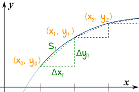
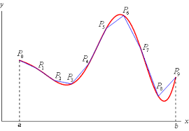
That is, the action is a functional of the Lagrangian. The Euler-Lagrange method of extremizing the action is to calculate the variation in $S$ as the path $x^{\mu}(p)$ is varied by a small amount $\delta x^{\mu}(p)$ as shown in Fig. $5.5$; the extremum path is characterized by the vanishing of the variation, precisely analogous to the vanishing of a derivative of a function at its extremum. The variation in $S$ is calculated in a straight-forward way as follows,
$$
\begin{aligned}
\delta S &=\int_{i}^{f}\left[\frac{\partial L}{\partial x^{\alpha}} \delta x^{\alpha}+\frac{\partial L}{\partial \dot{x}^{\alpha}} \delta \dot{x}^{\alpha}\right] \mathrm{d} p \
&=\int_{i}^{f}\left[\frac{\partial L}{\partial x^{\alpha}} \delta x^{\alpha}+\frac{\mathrm{d}}{\mathrm{d} p}\left(\frac{\partial L}{\partial \dot{x}^{\alpha}} \delta x^{\alpha}\right)-\delta x^{\alpha} \frac{\mathrm{d}}{\mathrm{d} p}\left(\frac{\partial L}{\partial \dot{x}^{\alpha}}\right)\right] \mathrm{d} p \
&=\int_{i}^{f}\left[\frac{\partial L}{\partial x^{\alpha}}-\frac{\mathrm{d}}{\mathrm{d} p}\left(\frac{\partial L}{\partial \dot{x}^{\alpha}}\right)\right] \delta x^{\alpha} \mathrm{d} p+\left(\frac{\partial L}{\partial \dot{x}^{\alpha}} \delta \dot{x}^{\alpha}\right)_{i}^{f}
\end{aligned}
$$
where we have integrated by parts and used $\delta \dot{x}^{\propto}=\mathrm{d}\left(\delta x^{\alpha}\right) / \mathrm{d} p$. Since we consider only paths between fixed endpoints the last term in the last line above is zero. Since we consider any small variation $\delta x^{\alpha}$ the bracket in the integral must be identically zero, so we conclude
$$
\frac{\mathrm{d}}{\mathrm{d} p}\left(\frac{\partial L}{\partial \dot{x}^{\alpha}}\right)-\frac{\partial L}{\partial x^{\alpha}}=0
$$
These differential equations are called the Euler-Lagrange equations, and yield a curve for which the action is extremum.

物理代写|广义相对论代写General relativity代考|Christoffel Connections as Fictitious Forces

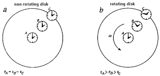
The Christoffel connections are actually familiar objects in classical mechanics, but they are seldom identified as such explicitly or seen from the geometrical point of view. They give rise to the well-known fictitious forces encountered in non-cartesian coordinate systems, rotating systems being a favorite example. To illustrate how this works we will study the motion of a particle in a potential in 3 -dimensional space with a general coordinate system using the Lagrangian formulation of classical mechanics. The manipulations are similar to those used in the preceding appendix and for discussing geodesics in the text.

Let the particle have a trajectory in three dimensions, with the position is given as a function of absolute (invariant) time by $x^{j}(t)$ in some coordinate system. Along this trajectory the line element represents the Euclidean distance
$$
\mathrm{ds}{ }^{2}=g_{i j} \mathrm{~d} x^{i} \mathrm{~d} x^{j} .
$$
Thus we may write the square of the velocity as
$$
v^{2}=g_{i j} \dot{x}^{i} \dot{x}^{j}, \quad \dot{x}^{i} \equiv \frac{\mathrm{d} x^{i}}{\mathrm{~d} t} .
$$
For a particle moving in a potential field the Lagrangian is generally taken to be the kinetic energy minus the potential energy,
$$
L=\frac{m}{2} v^{2}-V\left(x^{k}\right)=\frac{m}{2} g_{i j} \dot{x}^{i} \dot{x}^{j}-V\left(x^{k}\right) .
$$
Note the similarity of this to the function $T$ which we used in discussing geodesics. Lagrangian mechanics is based on the postulate that the action, the integral of $L$, is extremized for the correct trajectory. That is
$$
\delta S=0, \quad S=\int_{i}^{f} L \mathrm{~d} t=\int_{i}^{f}\left[\frac{m}{2} g_{i j} \dot{x}^{i} \dot{x}^{j}-V\left(x^{k}\right)\right] \mathrm{d} t .
$$
Extremizing the action we are led to the Euler-Lagrange equations as in our derivation of the geodesic equation, but now we also have a potential energy term. The EulerLagrange equations are obtained as usual, and are,

$\frac{\partial L}{\partial \dot{x}^{i}}=m g_{i j} \dot{x}^{j}, \quad \frac{\mathrm{d}}{\mathrm{d} t} \frac{\partial L}{\partial \dot{x}^{i}}=m\left(g_{i j} \ddot{x}^{j}+g_{i j, k} \dot{x}^{j} \dot{x}^{k}\right)$
$\frac{\partial L}{\partial x^{i}}=\frac{m}{2} g_{i j, k} \dot{x}^{j} \dot{x}^{k}-\frac{\partial V}{\partial x^{i}}$
$m\left(g_{i j} \ddot{x}^{j}+g_{i j, k} \dot{x}^{j} \dot{x}^{k}-\frac{1}{2} g_{j k, i} \dot{x}^{j} \dot{x}^{k}\right)+\frac{\partial V}{\partial x^{i}}=0$

广义相对论代考

物理代写|广义相对论代写General relativity代考|A Special Coordinate System

回想一下，在第一章。4 我们陈述了签名定理，即在任何时候磷存在一个特殊的坐标系，其中度量是对角的并且对角元素等于 1 或−1或 0 。特殊系统可以通过线性变换得到。这种度量形式称为 Cayley-Sylvester 规范形式。我们在附录 4.1（Perlis 1952）中证明了二维情况下的定理。

在本章中，我们获得了另一个特殊的坐标系，测地线系统，其中仿射连接在任何给定点都消失了磷. 如果连接为零，那么根据 Christoffel 连接 (5.19) 的定义，这显然意味着度量的一阶导数也必须为零。事实上，我们可以将这些变换结合起来，对于任何给定的点磷找到一个坐标系，其中度量具有 Cayley-Sylvester 规范形式，并且一阶导数消失，因此连接消失。为此，我们只需将两个变换与点一起应用磷被认为是起源，

X¯j=大号ķjXķ+12一个jl一世(大号njXn)(大号米lX米). 
这大号array 对度量具有 Cayley-Sylvester 规范形式的系统进行转换，并且一个数组指定到测地线系统的转换。这样得到的坐标系非常特殊：轴是正交的，度量是洛伦兹，连接消失了，所以物理学在局部很像狭义相对论，但当然只是在附近的一个很小的区域内磷.

物理代写|广义相对论代写General relativity代考|The Extremum Problem

为了完整起见，我们简要回顾了变分法中最重要的问题之一，大多数物理学家都熟悉经典力学的拉格朗日公式（Goldstein 1980）。拉格朗日被假定为坐标和广义速度的给定函数，大号(Xλ,X˙一个). 数量小号称为动作然后定义为从固定初始点沿某条曲线的拉格朗日积分一世到一个固定的终点F,

小号=∫一世F大号(Xλ,X˙一个)dp,X˙一个≡dX一个dp
也就是说，动作是拉格朗日函数的。Euler-Lagrange 对动作进行极值化的方法是计算小号作为路径Xμ(p)有少量变化dXμ(p)如图所示。5.5; 极值路径的特征在于变化的消失，这与函数的导数在其极值处的消失非常相似。的变化小号以直接的方式计算如下，

d小号=∫一世F[∂大号∂X一个dX一个+∂大号∂X˙一个dX˙一个]dp =∫一世F[∂大号∂X一个dX一个+ddp(∂大号∂X˙一个dX一个)−dX一个ddp(∂大号∂X˙一个)]dp =∫一世F[∂大号∂X一个−ddp(∂大号∂X˙一个)]dX一个dp+(∂大号∂X˙一个dX˙一个)一世F
我们按零件集成并使用的地方dX˙∝=d(dX一个)/dp. 由于我们只考虑固定端点之间的路径，因此上面最后一行中的最后一项为零。因为我们考虑任何小的变化dX一个积分中的括号必须相同为零，所以我们得出结论

ddp(∂大号∂X˙一个)−∂大号∂X一个=0
这些微分方程称为欧拉-拉格朗日方程，并产生一条作用为极值的曲线。

物理代写|广义相对论代写General relativity代考|Christoffel Connections as Fictitious Forces

Christoffel 连接实际上是经典力学中熟悉的对象，但它们很少被明确地识别为此类对象或从几何角度来看。它们产生了在非笛卡尔坐标系中遇到的众所周知的虚拟力，旋转系统是一个最喜欢的例子。为了说明这是如何工作的，我们将使用经典力学的拉格朗日公式来研究粒子在具有一般坐标系的 3 维空间中的势能运动。操作类似于前面附录中使用的操作以及用于讨论文本中的测地线。

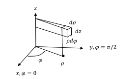
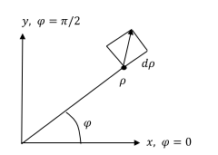
让粒子在三个维度上具有轨迹，位置是绝对（不变）时间的函数Xj(吨)在某个坐标系中。沿着这条轨迹线元素代表欧几里得距离

ds2=G一世j dX一世 dXj.
因此，我们可以将速度的平方写为

在2=G一世jX˙一世X˙j,X˙一世≡dX一世 d吨.
对于在势场中运动的粒子，拉格朗日通常被认为是动能减去势能，

大号=米2在2−在(Xķ)=米2G一世jX˙一世X˙j−在(Xķ).
注意 this 与函数的相似性吨我们在讨论测地线时使用了它。拉格朗日力学基于以下假设：作用，积分大号, 为正确的轨迹而极端化。那是

d小号=0,小号=∫一世F大号 d吨=∫一世F[米2G一世jX˙一世X˙j−在(Xķ)]d吨.
极端化我们得到欧拉-拉格朗日方程的作用，就像我们推导测地线方程一样，但现在我们还有一个势能项。EulerLagrange 方程是照常获得的，并且是，

∂大号∂X˙一世=米G一世jX˙j,dd吨∂大号∂X˙一世=米(G一世jX¨j+G一世j,ķX˙jX˙ķ)
∂大号∂X一世=米2G一世j,ķX˙jX˙ķ−∂在∂X一世
米(G一世jX¨j+G一世j,ķX˙jX˙ķ−12Gjķ,一世X˙jX˙ķ)+∂在∂X一世=0

统计代写请认准statistics-lab™. statistics-lab™为您的留学生涯保驾护航。

金融工程代写

金融工程是使用数学技术来解决金融问题。金融工程使用计算机科学、统计学、经济学和应用数学领域的工具和知识来解决当前的金融问题，以及设计新的和创新的金融产品。

非参数统计代写

非参数统计指的是一种统计方法，其中不假设数据来自于由少数参数决定的规定模型；这种模型的例子包括正态分布模型和线性回归模型。

广义线性模型代考

广义线性模型（GLM）归属统计学领域，是一种应用灵活的线性回归模型。该模型允许因变量的偏差分布有除了正态分布之外的其它分布。

术语 广义线性模型（GLM）通常是指给定连续和/或分类预测因素的连续响应变量的常规线性回归模型。它包括多元线性回归，以及方差分析和方差分析（仅含固定效应）。

有限元方法代写

有限元方法（FEM）是一种流行的方法，用于数值解决工程和数学建模中出现的微分方程。典型的问题领域包括结构分析、传热、流体流动、质量运输和电磁势等传统领域。

有限元是一种通用的数值方法，用于解决两个或三个空间变量的偏微分方程（即一些边界值问题）。为了解决一个问题，有限元将一个大系统细分为更小、更简单的部分，称为有限元。这是通过在空间维度上的特定空间离散化来实现的，它是通过构建对象的网格来实现的：用于求解的数值域，它有有限数量的点。边界值问题的有限元方法表述最终导致一个代数方程组。该方法在域上对未知函数进行逼近。[1] 然后将模拟这些有限元的简单方程组合成一个更大的方程系统，以模拟整个问题。然后，有限元通过变化微积分使相关的误差函数最小化来逼近一个解决方案。

tatistics-lab作为专业的留学生服务机构，多年来已为美国、英国、加拿大、澳洲等留学热门地的学生提供专业的学术服务，包括但不限于Essay代写，Assignment代写，Dissertation代写，Report代写，小组作业代写，Proposal代写，Paper代写，Presentation代写，计算机作业代写，论文修改和润色，网课代做，exam代考等等。写作范围涵盖高中，本科，研究生等海外留学全阶段，辐射金融，经济学，会计学，审计学，管理学等全球99%专业科目。写作团队既有专业英语母语作者，也有海外名校硕博留学生，每位写作老师都拥有过硬的语言能力，专业的学科背景和学术写作经验。我们承诺100%原创，100%专业，100%准时，100%满意。

随机分析代写

随机微积分是数学的一个分支，对随机过程进行操作。它允许为随机过程的积分定义一个关于随机过程的一致的积分理论。这个领域是由日本数学家伊藤清在第二次世界大战期间创建并开始的。

时间序列分析代写

随机过程，是依赖于参数的一组随机变量的全体，参数通常是时间。 随机变量是随机现象的数量表现，其时间序列是一组按照时间发生先后顺序进行排列的数据点序列。通常一组时间序列的时间间隔为一恒定值（如1秒，5分钟，12小时，7天，1年），因此时间序列可以作为离散时间数据进行分析处理。研究时间序列数据的意义在于现实中，往往需要研究某个事物其随时间发展变化的规律。这就需要通过研究该事物过去发展的历史记录，以得到其自身发展的规律。

回归分析代写

多元回归分析渐进（Multiple Regression Analysis Asymptotics）属于计量经济学领域，主要是一种数学上的统计分析方法，可以分析复杂情况下各影响因素的数学关系，在自然科学、社会和经济学等多个领域内应用广泛。

MATLAB代写

MATLAB 是一种用于技术计算的高性能语言。它将计算、可视化和编程集成在一个易于使用的环境中，其中问题和解决方案以熟悉的数学符号表示。典型用途包括：数学和计算算法开发建模、仿真和原型制作数据分析、探索和可视化科学和工程图形应用程序开发，包括图形用户界面构建MATLAB 是一个交互式系统，其基本数据元素是一个不需要维度的数组。这使您可以解决许多技术计算问题，尤其是那些具有矩阵和向量公式的问题，而只需用 C 或 Fortran 等标量非交互式语言编写程序所需的时间的一小部分。MATLAB 名称代表矩阵实验室。MATLAB 最初的编写目的是提供对由 LINPACK 和 EISPACK 项目开发的矩阵软件的轻松访问，这两个项目共同代表了矩阵计算软件的最新技术。MATLAB 经过多年的发展，得到了许多用户的投入。在大学环境中，它是数学、工程和科学入门和高级课程的标准教学工具。在工业领域，MATLAB 是高效研究、开发和分析的首选工具。MATLAB 具有一系列称为工具箱的特定于应用程序的解决方案。对于大多数 MATLAB 用户来说非常重要，工具箱允许您学习和应用专业技术。工具箱是 MATLAB 函数（M 文件）的综合集合，可扩展 MATLAB 环境以解决特定类别的问题。可用工具箱的领域包括信号处理、控制系统、神经网络、模糊逻辑、小波、仿真等。

R语言代写	问卷设计与分析代写
PYTHON代写	回归分析与线性模型代写
MATLAB代写	方差分析与试验设计代写
STATA代写	机器学习/统计学习代写
SPSS代写	计量经济学代写
EVIEWS代写	时间序列分析代写
EXCEL代写	深度学习代写
SQL代写	各种数据建模与可视化代写

如果你也在 怎样代写广义相对论General relativity这个学科遇到相关的难题，请随时右上角联系我们的24/7代写客服。

广义相对论是阿尔伯特-爱因斯坦在1907至1915年间提出的引力理论。广义相对论说，观察到的质量之间的引力效应是由它们对时空的扭曲造成的。

statistics-lab™ 为您的留学生涯保驾护航 在代写广义相对论General relativity方面已经树立了自己的口碑, 保证靠谱, 高质且原创的统计Statistics代写服务。我们的专家在代写广义相对论General relativity代写方面经验极为丰富，各种代写广义相对论General relativity相关的作业也就用不着说。

我们提供的广义相对论General relativity及其相关学科的代写，服务范围广, 其中包括但不限于:

• Statistical Inference 统计推断
• Statistical Computing 统计计算
• Advanced Probability Theory 高等概率论
• Advanced Mathematical Statistics 高等数理统计学
• (Generalized) Linear Models 广义线性模型
• Statistical Machine Learning 统计机器学习
• Longitudinal Data Analysis 纵向数据分析
• Foundations of Data Science 数据科学基础

物理代写|广义相对论代写General relativity代考|Geodesics as Self-parallel Curves

We now know how to displace a vector to a nearby point so that it remains parallel to itself in the general sense defined in the preceding two sections. We may use this to define and study the idea of a generalized straight line or geodesic. Our definition of a geodesic stems naturally from classical Euclidean geometry and intuition. Suppose we have a curve $C$ specified by giving the coordinates as functions of some scalar parameter $p$ which labels points on $C$,
Curve $C: x^{\mu}=x^{\mu}(p)$
We call $C$ a geodesic if it is everywhere parallel to itself; this means that if we parallel displace a tangent vector along $C$ then it remains a tangent vector.

This definition leads to a differential equation for the geodesic. Call the tangent vector $t^{\alpha}(p)$ at $p$. We parallel displace it along the curve to a nearby point labeled $p^{\prime}$ at a coordinate distance $\mathrm{d} x^{\alpha}$ to obtain
$$
t^{* \alpha}\left(p^{\prime}\right)=t^{\alpha}(p)-\Gamma_{\beta \gamma}^{\alpha} \mathrm{d} x^{\beta} t^{\gamma}(p)
$$
The actual tangent at $p^{\prime}$ may be obtained from that at $p$ by a Taylor Series expansion
$$
t^{\alpha}\left(p^{\prime}\right)=t^{\alpha}(p)+\frac{\mathrm{d} t^{\alpha}}{\mathrm{d} p} \mathrm{~d} p
$$
By our above definition of a geodesic the parallel displaced tangent vector in (5.23) is to be equal to the actual tangent vector in $(5.24)$, so that
$$
\frac{\mathrm{d} t^{\alpha}}{\mathrm{d} p} \mathrm{~d} p=-\Gamma_{\beta \gamma}^{\alpha} \mathrm{d} x^{\beta} t^{\gamma}
$$
We may choose the curve parameter $p$ to be the curve length, that is $\mathrm{d} p=\mathrm{d} s$, and use the normalized position derivative as an obvious tangent vector, normalized to unity,
$$
t^{\beta}=\frac{\mathrm{d} x^{\beta}}{\mathrm{d} s}
$$
Substituting this into (5.25) we obtain a differential equation for the geodesic
$$
\frac{\mathrm{d}^{2} x^{\alpha}}{\mathrm{d} s^{2}}+\Gamma_{\beta \gamma}^{\alpha} \frac{\mathrm{d} x^{\beta}}{\mathrm{d} s} \frac{\mathrm{d} x^{\gamma}}{\mathrm{d} s}=0
$$

物理代写|广义相对论代写General relativity代考|Geodesics as Extremum Curves

The self-parallel definition of a geodesic is one of several equivalent ones. In Euclidean geometry a straight line is the shortest distance between two given points. This property can be generalized to give the following definition of a geodesic: let the curve $C$ have length $s$ between two fixed points; then $C$ is a geodesic if the length $s$ is an extremum, that is it is either the shortest or longest among all nearby curves. We will show that this definition leads to the differential equation (5.28) and is equivalent to the self-parallel definition. The extremum calculation is a problem in the calculus of variations, well-known in classical mechanics. If the reader is not familiar with such problems and the Euler-Lagrange method of solution he should first consult Appendix $2 .$
As before the curve $C$ is denoted by
$$
\text { Curve } C: x^{\mu}=x^{\mu}(p) \text {. }
$$
Here $p$ is an invariant parameter, which may be the arc length of the curve but need not be. This is shown schematically in Fig. $5.5$.
The line element along the curve and the arc length $s$ can be written as

$$
\begin{gathered}
\mathrm{d} s^{2}=g_{\alpha \beta} \mathrm{d} x^{\alpha} \mathrm{d} x^{\beta}=g_{\alpha \beta} \dot{x}^{\alpha} \dot{x}^{\beta} \mathrm{d} p^{2} \equiv T\left(x^{\lambda}, \dot{x}^{\kappa}\right) \mathrm{d} p^{2}, \quad \dot{x}^{\kappa} \equiv \frac{\mathrm{d} x^{\kappa}}{\mathrm{d} p} \
s=\int_{i}^{f} \sqrt{g_{\alpha \beta} \dot{x}^{\alpha} \dot{x}^{\beta}} \mathrm{d} p=\int_{i}^{f} \sqrt{T\left(x^{\lambda}, \dot{x}^{\kappa}\right)} \mathrm{d} p
\end{gathered}
$$
where we have assumed the line element $\mathrm{d} s^{2}$ is positive. Finding the extremum of this arc length integral is a standard problem in the calculus of variations and solvable by the Euler-Lagrange method. Indeed it is the analog of a classical mechanics problem with a Lagrangian
$$
L=\sqrt{T\left(x^{\lambda}, \dot{x}^{x}\right)}, \quad T\left(x^{\lambda}, \dot{x}^{\kappa}\right) \equiv g_{\alpha \beta} \dot{x}^{\alpha} \dot{x}^{\beta} .
$$

物理代写|广义相对论代写General relativity代考|Affine Connections, Abstract View

Let us see how we may motivate and interpret the coefficients of affine connection using the abstract view introduced in Sect. 4.3. Recall that a vector may be expanded in a coordinate basis, that is vectors aligned along the coordinate axes, according to
$$
\vec{V}=V^{j} \vec{e}{j}, \quad \vec{e}{j}=\text { coordinate basis. }
$$
If we think of moving the vector to a nearby point it will change due to a change in its components and also a change in the basis vectors,
$$
\mathrm{d} \vec{V}=\vec{e}{i} \mathrm{~d} V^{i}+V^{j} \mathrm{~d} \vec{e}{j}
$$
As we discussed previously the vector spaces associated with different points in a Riemann space are ab initio independent. As such it is necessary to postulate a way to relate them. This leads to the idea of vector transplantation and the specific version of transplantation called parallel displacement that we discussed in Sects. $5.1$ and 5.3. We can think of this in the present abstract view as giving an effective change in the coordinate basis, which we assume is a bilinear expression in the basis vectors and the coordinate displacement; it is a rather compelling assumption. That is we postulate
$$
\mathrm{d} \vec{e}{j}=\Gamma{k j}^{i}\left(\vec{e}_{i} \mathrm{~d} x^{k}\right) .
$$

广义相对论代考

物理代写|广义相对论代写General relativity代考|Geodesics as Self-parallel Curves

我们现在知道如何将向量移动到附近的点，以使其保持与前两节定义的一般意义上的自身平行。我们可以用它来定义和研究广义直线或测地线的概念。我们对测地线的定义自然源于经典的欧几里得几何和直觉。假设我们有一条曲线C通过将坐标指定为某个标量参数的函数p哪些标签指向C,
曲线C:Xμ=Xμ(p)
我们称之为C如果它处处平行于自身，则为测地线；这意味着如果我们沿平行位移一个切向量C那么它仍然是一个切向量。

该定义导致测地线的微分方程。调用切向量吨一个(p)在p. 我们将它沿曲线平行移动到附近标记为的点p′在坐标距离dX一个获得

吨∗一个(p′)=吨一个(p)−ΓbC一个dXb吨C(p)
实际切线在p′可以从中获得p由泰勒级数展开

吨一个(p′)=吨一个(p)+d吨一个dp dp
根据我们上面对测地线的定义，(5.23) 中的平行位移切向量等于(5.24)， 以便

d吨一个dp dp=−ΓbC一个dXb吨C
我们可以选择曲线参数p为曲线长度，即dp=ds，并使用归一化的位置导数作为明显的切向量，归一化为单位，

吨b=dXbds
将其代入 (5.25) 我们得到测地线的微分方程

d2X一个ds2+ΓbC一个dXbdsdXCds=0

物理代写|广义相对论代写General relativity代考|Geodesics as Extremum Curves

测地线的自平行定义是几个等效定义之一。在欧几里得几何中，直线是两个给定点之间的最短距离。这个性质可以概括为给出测地线的以下定义：让曲线C有长度s两个固定点之间；然后C如果长度是测地线s是一个极值，即它是所有附近曲线中最短或最长的。我们将证明这个定义导致了微分方程（5.28）并且等价于自平行定义。极值计算是变分法中的一个问题，在经典力学中是众所周知的。如果读者不熟悉此类问题和欧拉-拉格朗日解法，应先查阅附录2.
和之前的曲线一样C表示为

 曲线 C:Xμ=Xμ(p). 
这里p是一个不变的参数，它可以是曲线的弧长，但不一定是。这在图 1 中示意性地显示。5.5.
沿曲线的线元素和弧长s可以写成

ds2=G一个bdX一个dXb=G一个bX˙一个X˙bdp2≡吨(Xλ,X˙ķ)dp2,X˙ķ≡dXķdp s=∫一世FG一个bX˙一个X˙bdp=∫一世F吨(Xλ,X˙ķ)dp
我们假设线元素ds2是积极的。求弧长积分的极值是变分法中的一个标准问题，可以通过欧拉-拉格朗日方法求解。实际上，它是具有拉格朗日算子的经典力学问题的类比

大号=吨(Xλ,X˙X),吨(Xλ,X˙ķ)≡G一个bX˙一个X˙b.

物理代写|广义相对论代写General relativity代考|Affine Connections, Abstract View

让我们看看如何使用 Sect 中介绍的抽象视图来激发和解释仿射连接系数。4.3. 回想一下，向量可以在坐标基础上展开，即沿着坐标轴对齐的向量，根据

在→=在j和→j,和→j= 坐标基础。 
如果我们考虑将向量移动到附近的点，它将由于其分量的变化以及基向量的变化而发生变化，

d在→=和→一世 d在一世+在j d和→j
正如我们之前所讨论的，与黎曼空间中的不同点相关的向量空间是从头算独立的。因此，有必要假设一种将它们联系起来的方法。这导致了向量移植的想法以及我们在 Sects 中讨论的称为平行位移的特定移植版本。5.1和 5.3。在目前的抽象视图中，我们可以认为这是对坐标基础的有效改变，我们假设它是基础向量和坐标位移的双线性表达式；这是一个相当令人信服的假设。那就是我们假设

d和→j=Γķj一世(和→一世 dXķ).

统计代写请认准statistics-lab™. statistics-lab™为您的留学生涯保驾护航。

金融工程代写

金融工程是使用数学技术来解决金融问题。金融工程使用计算机科学、统计学、经济学和应用数学领域的工具和知识来解决当前的金融问题，以及设计新的和创新的金融产品。

非参数统计代写

非参数统计指的是一种统计方法，其中不假设数据来自于由少数参数决定的规定模型；这种模型的例子包括正态分布模型和线性回归模型。

广义线性模型代考

广义线性模型（GLM）归属统计学领域，是一种应用灵活的线性回归模型。该模型允许因变量的偏差分布有除了正态分布之外的其它分布。

术语 广义线性模型（GLM）通常是指给定连续和/或分类预测因素的连续响应变量的常规线性回归模型。它包括多元线性回归，以及方差分析和方差分析（仅含固定效应）。

有限元方法代写

有限元方法（FEM）是一种流行的方法，用于数值解决工程和数学建模中出现的微分方程。典型的问题领域包括结构分析、传热、流体流动、质量运输和电磁势等传统领域。

有限元是一种通用的数值方法，用于解决两个或三个空间变量的偏微分方程（即一些边界值问题）。为了解决一个问题，有限元将一个大系统细分为更小、更简单的部分，称为有限元。这是通过在空间维度上的特定空间离散化来实现的，它是通过构建对象的网格来实现的：用于求解的数值域，它有有限数量的点。边界值问题的有限元方法表述最终导致一个代数方程组。该方法在域上对未知函数进行逼近。[1] 然后将模拟这些有限元的简单方程组合成一个更大的方程系统，以模拟整个问题。然后，有限元通过变化微积分使相关的误差函数最小化来逼近一个解决方案。

tatistics-lab作为专业的留学生服务机构，多年来已为美国、英国、加拿大、澳洲等留学热门地的学生提供专业的学术服务，包括但不限于Essay代写，Assignment代写，Dissertation代写，Report代写，小组作业代写，Proposal代写，Paper代写，Presentation代写，计算机作业代写，论文修改和润色，网课代做，exam代考等等。写作范围涵盖高中，本科，研究生等海外留学全阶段，辐射金融，经济学，会计学，审计学，管理学等全球99%专业科目。写作团队既有专业英语母语作者，也有海外名校硕博留学生，每位写作老师都拥有过硬的语言能力，专业的学科背景和学术写作经验。我们承诺100%原创，100%专业，100%准时，100%满意。

随机分析代写

随机微积分是数学的一个分支，对随机过程进行操作。它允许为随机过程的积分定义一个关于随机过程的一致的积分理论。这个领域是由日本数学家伊藤清在第二次世界大战期间创建并开始的。

时间序列分析代写

随机过程，是依赖于参数的一组随机变量的全体，参数通常是时间。 随机变量是随机现象的数量表现，其时间序列是一组按照时间发生先后顺序进行排列的数据点序列。通常一组时间序列的时间间隔为一恒定值（如1秒，5分钟，12小时，7天，1年），因此时间序列可以作为离散时间数据进行分析处理。研究时间序列数据的意义在于现实中，往往需要研究某个事物其随时间发展变化的规律。这就需要通过研究该事物过去发展的历史记录，以得到其自身发展的规律。

回归分析代写

多元回归分析渐进（Multiple Regression Analysis Asymptotics）属于计量经济学领域，主要是一种数学上的统计分析方法，可以分析复杂情况下各影响因素的数学关系，在自然科学、社会和经济学等多个领域内应用广泛。

MATLAB代写

MATLAB 是一种用于技术计算的高性能语言。它将计算、可视化和编程集成在一个易于使用的环境中，其中问题和解决方案以熟悉的数学符号表示。典型用途包括：数学和计算算法开发建模、仿真和原型制作数据分析、探索和可视化科学和工程图形应用程序开发，包括图形用户界面构建MATLAB 是一个交互式系统，其基本数据元素是一个不需要维度的数组。这使您可以解决许多技术计算问题，尤其是那些具有矩阵和向量公式的问题，而只需用 C 或 Fortran 等标量非交互式语言编写程序所需的时间的一小部分。MATLAB 名称代表矩阵实验室。MATLAB 最初的编写目的是提供对由 LINPACK 和 EISPACK 项目开发的矩阵软件的轻松访问，这两个项目共同代表了矩阵计算软件的最新技术。MATLAB 经过多年的发展，得到了许多用户的投入。在大学环境中，它是数学、工程和科学入门和高级课程的标准教学工具。在工业领域，MATLAB 是高效研究、开发和分析的首选工具。MATLAB 具有一系列称为工具箱的特定于应用程序的解决方案。对于大多数 MATLAB 用户来说非常重要，工具箱允许您学习和应用专业技术。工具箱是 MATLAB 函数（M 文件）的综合集合，可扩展 MATLAB 环境以解决特定类别的问题。可用工具箱的领域包括信号处理、控制系统、神经网络、模糊逻辑、小波、仿真等。

R语言代写	问卷设计与分析代写
PYTHON代写	回归分析与线性模型代写
MATLAB代写	方差分析与试验设计代写
STATA代写	机器学习/统计学习代写
SPSS代写	计量经济学代写
EVIEWS代写	时间序列分析代写
EXCEL代写	深度学习代写
SQL代写	各种数据建模与可视化代写

如果你也在 怎样代写广义相对论General relativity这个学科遇到相关的难题，请随时右上角联系我们的24/7代写客服。

广义相对论是阿尔伯特-爱因斯坦在1907至1915年间提出的引力理论。广义相对论说，观察到的质量之间的引力效应是由它们对时空的扭曲造成的。

statistics-lab™ 为您的留学生涯保驾护航 在代写广义相对论General relativity方面已经树立了自己的口碑, 保证靠谱, 高质且原创的统计Statistics代写服务。我们的专家在代写广义相对论General relativity代写方面经验极为丰富，各种代写广义相对论General relativity相关的作业也就用不着说。

我们提供的广义相对论General relativity及其相关学科的代写，服务范围广, 其中包括但不限于:

• Statistical Inference 统计推断
• Statistical Computing 统计计算
• Advanced Probability Theory 高等概率论
• Advanced Mathematical Statistics 高等数理统计学
• (Generalized) Linear Models 广义线性模型
• Statistical Machine Learning 统计机器学习
• Longitudinal Data Analysis 纵向数据分析
• Foundations of Data Science 数据科学基础

物理代写|广义相对论代写General relativity代考|Affine Connections, Component View

Most of our considerations in Chap. 4 involved vectors and tensors associated with a single point. Now we study how to compare vectors and tensors at different points in a Riemann space, and how to move them (Misner 1973; Adler 1975; Schutz 2009). This is necessary in order to study tensor fields, that is tensors defined as functions of position in regions of space; these fields may be denoted for example as
$$
\phi\left(x^{\mu}\right) \text { scalar, } V^{\propto}\left(x^{\mu}\right) \text { vector, } T^{\propto \beta}\left(x^{\mu}\right) 2 \text { nd rank tensor. }
$$
This is not a trivial process since vector spaces at different points in a Riemann space are a priori independent and any connection between them requires analysis. The key concept is that of affine connections, for which we will motivate a definition; then on the basis of the definition we may obtain their transformation law.

Much of the work in this chapter is based on the classic component view, but we will relate it to the abstract view in the last section.

Consider first a constant vector field in Euclidean 3-space with Cartesian coordinates; the definition of such a constant vector field is obviously that the components are constant, as shown in Fig. 5.1a. But it is also clear that in spherical coordinates constant components do not correspond to what we think of as a constant vector field, as in Fig. 5.1b. Clearly, we should not define a constant vector field as one with constant components. The terms “constant” and “parallel” remain to be defined precisely. The proper definition of a constant vector field will introduce the concept of affine connections as an elegant generalization of the notion of parallel vectors.

物理代写|广义相对论代写General relativity代考|Transformation of the Affine Connections

The law of vector transplantation introduced in (5.5) is extremely general since there are no restrictions on the connections. Remarkably, from only the above definition

of vector transplantation we may obtain the transformation law for the connections, which we will find are not tensors. Moreover several theorems that result from the transformation law are basic and important for both mathematics and physics.

To find the transformation law we make the natural demand that a vector remains a vector as it is transplanted to a nearby point: that is it must obey the transformation law (4.14) at both $P$ and $P^{\prime}$. The transplanted vector, at $P^{\prime}$ in the barred and unbarred coordinate systems, is
$$
V^{* i}=V^{i}-\Gamma_{p q}^{i} \mathrm{~d} x^{p} V^{q}, \quad \bar{V}^{* j}=\bar{V}^{j}-\bar{\Gamma}{m n}^{j} \mathrm{~d} \bar{x}^{m} \bar{V}^{n} $$ Here the vector and connections on the right side of $(5.6)$ are evaluated at $P$. The transformation matrix at $P^{\prime}$ may be gotten with a Taylor series expansion from that at $P$ $$ \left(\frac{\partial \bar{x}^{j}}{\partial x^{i}}\right){P}=\left(\frac{\partial \bar{x}^{j}}{\partial x^{i}}\right){P}+\frac{\partial}{\partial x^{l}}\left(\frac{\partial \bar{x}^{j}}{\partial x^{i}}\right){P} \mathrm{~d} x^{l}=\left(\frac{\partial \bar{x}^{j}}{\partial x^{i}}\right){P}+\left(\frac{\partial^{2} \bar{x}^{j}}{\partial x^{l} \partial x^{i}}\right){P} \mathrm{~d} x^{l} .
$$
We use these expressions and impose the vector transformation law on the vector at $P^{\prime}$
$$
\begin{aligned}
&\bar{V}^{* j}=\left(\frac{\partial \bar{x}^{j}}{\partial x^{l}}\right){P^{\prime}} V^{* l} \text { so } \ &\bar{V}^{j}-\bar{\Gamma}{m n}^{j} \mathrm{~d} \bar{x}^{m} \bar{V}^{n}=\left[\left(\frac{\partial \bar{x}^{j}}{\partial x^{i}}\right){P}+\left(\frac{\partial^{2} \bar{x}^{j}}{\partial x^{l} \partial x^{i}}\right){P} \mathrm{~d} x^{l}\right]\left[V^{i}-\Gamma_{p q}^{i} \mathrm{~d} x^{p} V^{q}\right] \
&=\left(\frac{\partial \bar{x}^{j}}{\partial x^{i}}\right){P} V^{i}-\left(\frac{\partial \bar{x}^{j}}{\partial x^{i}}\right){P}^{\Gamma_{p q}^{i}} \mathrm{~d} x^{p} V^{q}+\left(\frac{\partial^{2} \bar{x}^{j}}{\partial x^{l} \partial x^{i}}\right)_{P} \mathrm{~d} x^{l} V^{i}
\end{aligned}
$$

物理代写|广义相对论代写General relativity代考|Parallel Displacement

The law of vector transplantation (5.5) introduced in the preceding section provides a way to compare vectors at different nearby points in space. By repeated iterations we could also compare vectors at widely separated points. Our considerations have so far been quite general and we made no assumptions about how the connections might be specified. We now specialize to obtain the specific connections used in relativity theory; this provides a strikingly elegant generalization of the idea of moving a vector parallel to itself in Euclidean geometry, and is called parallel displacement. Parallel displacement is basic to the idea and definition of space curvature that we will develop in Chap. 8. It also allows us to define geodesic curves, which are the generalization of straight lines to general Riemann spaces.

Suppose that we transplant two vectors to a nearby point using the law of vector transplantation. There is no a priori reason that the inner product of the two will remain unchanged; however we may consider this to be a naturally compelling demand to be imposed so as to make the transplantation analogous to the parallel displacement of vectors in Euclidean geometry. In the special case of Euclidean space the demand for parallelism implies that the lengths of various vectors and the angles between them remain unchanged as they are transplanted. We thus impose this demand and refer to this special case of vector transplantation as generalized parallel displacement, or simply parallel displacement for brevity. Remarkably, the connections are then

determined uniquely by the metric. Figure $5.3$ shows the scenario for the parallel displacement of two vectors.

The derivation of the affine connections is conceptually simple and involves only slightly tedious algebra. The demand that the inner product of the two vectors be unchanged under vector transplantation may be expressed as
$$
\mathrm{d}\left(\xi^{j} \eta^{k} g_{j k}\right)^{*}=0
$$

广义相对论代考

物理代写|广义相对论代写General relativity代考|Affine Connections, Component View

我们在第一章中的大部分考虑。4 涉及与单个点相关的向量和张量。现在我们研究如何比较黎曼空间中不同点的向量和张量，以及如何移动它们（Misner 1973；Adler 1975；Schutz 2009）。这对于研究张量场是必要的，张量被定义为空间区域中位置的函数；例如，这些字段可以表示为

φ(Xμ) 标量， 在∝(Xμ) 向量， 吨∝b(Xμ)2 nd 秩张量。 
这不是一个简单的过程，因为黎曼空间中不同点的向量空间是先验独立的，并且它们之间的任何联系都需要分析。关键概念是仿射连接的概念，我们将对此进行定义；那么根据定义我们可以得到它们的变换规律。

本章的大部分工作都基于经典的组件视图，但我们将在最后一节中将其与抽象视图联系起来。

首先考虑具有笛卡尔坐标的欧几里得 3 空间中的常数向量场；这样一个常数向量场的定义显然是分量是常数，如图 5.1a 所示。但同样清楚的是，在球坐标系中，常数分量并不对应于我们认为的常数矢量场，如图 5.1b 所示。显然，我们不应该将恒定矢量场定义为具有恒定分量的场。术语“恒定”和“平行”仍有待精确定义。常数向量场的正确定义将引入仿射连接的概念作为并行向量概念的优雅概括。

物理代写|广义相对论代写General relativity代考|Transformation of the Affine Connections

（5.5）中引入的向量移植定律非常普遍，因为对连接没有限制。值得注意的是，仅从上述定义

在向量移植的过程中，我们可以获得连接的变换定律，我们会发现它不是张量。此外，从变换定律得出的几个定理对于数学和物理学来说都是基本且重要的。

为了找到变换定律，我们提出一个向量在移植到附近点时仍然是向量的自然要求：即它必须在两个点都遵守变换定律 (4.14)磷和磷′. 移植的载体，在磷′在 barred 和 unbarred 坐标系中，是

在∗一世=在一世−Γpq一世 dXp在q,在¯∗j=在¯j−Γ¯米nj dX¯米在¯n这里右边的向量和连接(5.6)被评估在磷. 变换矩阵磷′可以通过泰勒级数展开得到磷

(∂X¯j∂X一世)磷=(∂X¯j∂X一世)磷+∂∂Xl(∂X¯j∂X一世)磷 dXl=(∂X¯j∂X一世)磷+(∂2X¯j∂Xl∂X一世)磷 dXl.
我们使用这些表达式并在向量上施加向量变换定律磷′

在¯∗j=(∂X¯j∂Xl)磷′在∗l 所以  在¯j−Γ¯米nj dX¯米在¯n=[(∂X¯j∂X一世)磷+(∂2X¯j∂Xl∂X一世)磷 dXl][在一世−Γpq一世 dXp在q] =(∂X¯j∂X一世)磷在一世−(∂X¯j∂X一世)磷Γpq一世 dXp在q+(∂2X¯j∂Xl∂X一世)磷 dXl在一世

物理代写|广义相对论代写General relativity代考|Parallel Displacement

上一节介绍的向量移植定律（5.5）提供了一种比较空间中不同附近点的向量的方法。通过重复迭代，我们还可以比较相距较远的点的向量。到目前为止，我们的考虑非常笼统，我们没有对如何指定连接做出任何假设。我们现在专门获取相对论中使用的特定联系；这为在欧几里得几何中平行于自身移动向量的想法提供了一个非常优雅的概括，称为平行位移。平行位移是空间曲率概念和定义的基础，我们将在第 1 章中阐述。8. 它还允许我们定义测地线曲线，即直线到一般黎曼空间的推广。

假设我们使用向量移植法则将两个向量移植到附近的点。两者的内积保持不变，没有先验的原因；然而，我们可以认为这是一个自然而然的强制要求，以便使移植类似于欧几里得几何中向量的平行位移。在欧几里得空间的特殊情况下，对平行度的要求意味着各种向量的长度和它们之间的角度在移植时保持不变。因此，我们强加了这一要求，并将向量移植的这种特殊情况称为广义平行位移，或为简洁起见简称为平行位移。值得注意的是，连接是

由度量唯一确定。数字5.3显示了两个向量平行位移的场景。

仿射连接的推导在概念上很简单，只涉及稍微繁琐的代数。两种载体在载体移植下内积不变的要求可表示为

d(Xj这ķGjķ)∗=0

统计代写请认准statistics-lab™. statistics-lab™为您的留学生涯保驾护航。

金融工程代写

金融工程是使用数学技术来解决金融问题。金融工程使用计算机科学、统计学、经济学和应用数学领域的工具和知识来解决当前的金融问题，以及设计新的和创新的金融产品。

非参数统计代写

非参数统计指的是一种统计方法，其中不假设数据来自于由少数参数决定的规定模型；这种模型的例子包括正态分布模型和线性回归模型。

广义线性模型代考

广义线性模型（GLM）归属统计学领域，是一种应用灵活的线性回归模型。该模型允许因变量的偏差分布有除了正态分布之外的其它分布。

术语 广义线性模型（GLM）通常是指给定连续和/或分类预测因素的连续响应变量的常规线性回归模型。它包括多元线性回归，以及方差分析和方差分析（仅含固定效应）。

有限元方法代写

有限元方法（FEM）是一种流行的方法，用于数值解决工程和数学建模中出现的微分方程。典型的问题领域包括结构分析、传热、流体流动、质量运输和电磁势等传统领域。

有限元是一种通用的数值方法，用于解决两个或三个空间变量的偏微分方程（即一些边界值问题）。为了解决一个问题，有限元将一个大系统细分为更小、更简单的部分，称为有限元。这是通过在空间维度上的特定空间离散化来实现的，它是通过构建对象的网格来实现的：用于求解的数值域，它有有限数量的点。边界值问题的有限元方法表述最终导致一个代数方程组。该方法在域上对未知函数进行逼近。[1] 然后将模拟这些有限元的简单方程组合成一个更大的方程系统，以模拟整个问题。然后，有限元通过变化微积分使相关的误差函数最小化来逼近一个解决方案。

tatistics-lab作为专业的留学生服务机构，多年来已为美国、英国、加拿大、澳洲等留学热门地的学生提供专业的学术服务，包括但不限于Essay代写，Assignment代写，Dissertation代写，Report代写，小组作业代写，Proposal代写，Paper代写，Presentation代写，计算机作业代写，论文修改和润色，网课代做，exam代考等等。写作范围涵盖高中，本科，研究生等海外留学全阶段，辐射金融，经济学，会计学，审计学，管理学等全球99%专业科目。写作团队既有专业英语母语作者，也有海外名校硕博留学生，每位写作老师都拥有过硬的语言能力，专业的学科背景和学术写作经验。我们承诺100%原创，100%专业，100%准时，100%满意。

随机分析代写

随机微积分是数学的一个分支，对随机过程进行操作。它允许为随机过程的积分定义一个关于随机过程的一致的积分理论。这个领域是由日本数学家伊藤清在第二次世界大战期间创建并开始的。

时间序列分析代写

随机过程，是依赖于参数的一组随机变量的全体，参数通常是时间。 随机变量是随机现象的数量表现，其时间序列是一组按照时间发生先后顺序进行排列的数据点序列。通常一组时间序列的时间间隔为一恒定值（如1秒，5分钟，12小时，7天，1年），因此时间序列可以作为离散时间数据进行分析处理。研究时间序列数据的意义在于现实中，往往需要研究某个事物其随时间发展变化的规律。这就需要通过研究该事物过去发展的历史记录，以得到其自身发展的规律。

回归分析代写

多元回归分析渐进（Multiple Regression Analysis Asymptotics）属于计量经济学领域，主要是一种数学上的统计分析方法，可以分析复杂情况下各影响因素的数学关系，在自然科学、社会和经济学等多个领域内应用广泛。

MATLAB代写

MATLAB 是一种用于技术计算的高性能语言。它将计算、可视化和编程集成在一个易于使用的环境中，其中问题和解决方案以熟悉的数学符号表示。典型用途包括：数学和计算算法开发建模、仿真和原型制作数据分析、探索和可视化科学和工程图形应用程序开发，包括图形用户界面构建MATLAB 是一个交互式系统，其基本数据元素是一个不需要维度的数组。这使您可以解决许多技术计算问题，尤其是那些具有矩阵和向量公式的问题，而只需用 C 或 Fortran 等标量非交互式语言编写程序所需的时间的一小部分。MATLAB 名称代表矩阵实验室。MATLAB 最初的编写目的是提供对由 LINPACK 和 EISPACK 项目开发的矩阵软件的轻松访问，这两个项目共同代表了矩阵计算软件的最新技术。MATLAB 经过多年的发展，得到了许多用户的投入。在大学环境中，它是数学、工程和科学入门和高级课程的标准教学工具。在工业领域，MATLAB 是高效研究、开发和分析的首选工具。MATLAB 具有一系列称为工具箱的特定于应用程序的解决方案。对于大多数 MATLAB 用户来说非常重要，工具箱允许您学习和应用专业技术。工具箱是 MATLAB 函数（M 文件）的综合集合，可扩展 MATLAB 环境以解决特定类别的问题。可用工具箱的领域包括信号处理、控制系统、神经网络、模糊逻辑、小波、仿真等。

R语言代写	问卷设计与分析代写
PYTHON代写	回归分析与线性模型代写
MATLAB代写	方差分析与试验设计代写
STATA代写	机器学习/统计学习代写
SPSS代写	计量经济学代写
EVIEWS代写	时间序列分析代写
EXCEL代写	深度学习代写
SQL代写	各种数据建模与可视化代写

如果你也在 怎样代写广义相对论General relativity这个学科遇到相关的难题，请随时右上角联系我们的24/7代写客服。

广义相对论是阿尔伯特-爱因斯坦在1907至1915年间提出的引力理论。广义相对论说，观察到的质量之间的引力效应是由它们对时空的扭曲造成的。

statistics-lab™ 为您的留学生涯保驾护航 在代写广义相对论General relativity方面已经树立了自己的口碑, 保证靠谱, 高质且原创的统计Statistics代写服务。我们的专家在代写广义相对论General relativity代写方面经验极为丰富，各种代写广义相对论General relativity相关的作业也就用不着说。

我们提供的广义相对论General relativity及其相关学科的代写，服务范围广, 其中包括但不限于:

• Statistical Inference 统计推断
• Statistical Computing 统计计算
• Advanced Probability Theory 高等概率论
• Advanced Mathematical Statistics 高等数理统计学
• (Generalized) Linear Models 广义线性模型
• Statistical Machine Learning 统计机器学习
• Longitudinal Data Analysis 纵向数据分析
• Foundations of Data Science 数据科学基础

物理代写|广义相对论代写General relativity代考|Volume Elements

In general relativity we often need the integral of a scalar function, which itself is a scalar. The integral of a vector or tensor will not in general have a well-defined transformation law since it is not a quantity defined at a single point. Our task in this section is to obtain an expression for a volume element to be used when integrating a scalar function over all or part of a space.

The appropriate expression for a volume element in a general Riemann space can be obtained by first considering the special case of a diagonal metric and then generalizing to any metric using invariance arguments. For a diagonal metric in any number of dimensions we may write the line element as
$$
\mathrm{d} s^{2}=\sum_{i} g_{i i}\left(\mathrm{~d} x^{i}\right)^{2}, \quad \mathrm{~d} \ell_{i} \equiv \sqrt{g_{i i}} \mathrm{~d} x^{i}=\text { physical distance in } i \text { direction. }
$$
That is, as we discussed in Sect. $4.3$, the $\mathrm{d} \ell_{i}$ is a physical distance interval. (We assume for the moment that $g_{i i}$ is positive.) What is particularly nice is that this allows us to define a physically meaningful $n$-volume element in a clear and obvious

way, as the product of the physical distances,
$$
\mathrm{d} V_{n} \equiv \mathrm{d} \ell \ldots \mathrm{d} \ell_{n}=\sqrt{g_{11 \ldots g_{n n}}} \mathrm{~d} x^{1} \ldots \mathrm{d} x^{n}=\sqrt{|g|} d^{n} x, \ldots
$$
where $|g|$ denotes the determinant of the metric tensor. This last expression turns out to be general, except that one must use the absolute value of the determinant if the signature is negative.

To show that the expression $(4.76)$ is the correct volume element we prove the following theorem.

物理代写|广义相对论代写General relativity代考|Differential Manifolds

The term manifold occurs in more mathematically oriented work. A manifold is an open collection of points $P$ with useful properties for physics applications; because the collection is open there will be by definition a region around each point that is also in the manifold. The points in a 1 -dimensional manifold are in one to one correspondence with an open set of the reals; an open set of the reals is defined as a union of open intervals. Similarly the points in a 2 -dimensional manifold are in one to one correspondence with a pair of reals, and so forth for any dimension $n$. Thus an $n$-dimensional manifold is an open set of points that can be labeled by an $n$-tuple of reals in an open region, that is by coordinates.

A function of the manifold points $P$ can be defined in terms of a function of the coordinates as $f(P)=f\left(x^{k}\right)$. Continuous and differentiable functions are naturally of particular usefulness.

In general the labeling of the points in a manifold is not unique and several coordinate systems may be used to label a region of the manifold; they are often denoted as unprimed and primed, or unbarred and barred as we have done. If there is a differentiable and invertible transformation $\bar{x}^{k}=\bar{x}^{k}\left(x^{i}\right)$ between any two such coordinate systems we say that the manifold is differentiable. This means that a differentiable function of the points in the manifold corresponds to a continuous function in both coordinate systems.

Thus, in short, a manifold is simply the kind of space physics has used for centuries, defined a bit more carefully with an emphasis on coordinate systems and open sets.

物理代写|广义相对论代写General relativity代考|The Signature Theorem in Two Dimensions

The Signature Theorem states that one can find a linear transformation to a coordinate system in which the metric tensor is diagonal and has $1,-1$, or 0 as diagonal elements. We will illustrate the proof in two dimensions with signature $(1,1)$ for simplicity. This is clearly a matrix problem so we will use matrix notation rather than index notation. We need deal only with a single point. The transformation between the original system and a new barred system we write in matrix form as
$$
x=D \bar{x},
$$
where $D$ is a matrix to be determined. The metric $G$ transforms as a second rank tensor so its transformation in matrix form is
$$
\bar{G}=D^{\mathrm{T}} G D, \quad G=\left(\begin{array}{ll}
g_{11} & g_{12} \
g_{12} & g_{22}
\end{array}\right)
$$
We first make the metric diagonal by choosing the transformation matrix $D$ with a single parameter $b$ to be determined,
$$
D=\left(\begin{array}{ll}
1 & 0 \
b & 1
\end{array}\right)
$$
After the transformation the metric becomes
$$
\bar{G}=\left(\begin{array}{cc}
g_{11}+2 b g_{12}+b^{2} g_{22} & g_{12}+b g_{22} \
g_{12}+b g_{22} & g_{22}
\end{array}\right)
$$
We make this diagonal by choosing $b=-g_{12} / g_{22}$. Then we have

$$
\bar{G}=\left(\begin{array}{cc}
g_{11}-\left(g_{12}\right)^{2} / g_{22} & 0 \
0 & g_{22}
\end{array}\right)=\left(\begin{array}{cc}
\bar{g}{11} & 0 \ 0 & \bar{g}{22}
\end{array}\right)
$$
Notice that the 1,1 element of the matrix $\bar{G}$ is the determinate of $G$ divided by $g_{22}$; we will assume this is positive so that the signature will be $(1,1)$. (The reader should work out the case where it is negative and the signature is (1, -1) as in Exercise 4.7)
We next apply a second linear transformation to stretch the coordinates and make both diagonal elements of the metric equal to 1 . Specifically this is done with the obvious stretching matrix
$$
\left(\begin{array}{cc}
\sqrt{g}{11} & 0 \ 0 & \sqrt{\bar{g}{22}}
\end{array}\right)
$$

广义相对论代考

物理代写|广义相对论代写General relativity代考|Volume Elements

在广义相对论中，我们经常需要标量函数的积分，它本身就是一个标量。向量或张量的积分通常没有明确定义的变换定律，因为它不是在单个点上定义的量。我们在本节中的任务是获得在对全部或部分空间进行标量函数积分时要使用的体积元素的表达式。

一般黎曼空间中体积元素的适当表达式可以通过首先考虑对角度量的特殊情况，然后使用不变参数推广到任何度量来获得。对于任意维数的对角线度量，我们可以将线元素写为

ds2=∑一世G一世一世( dX一世)2, dℓ一世≡G一世一世 dX一世= 物理距离 一世 方向。 
也就是说，正如我们在 Sect 中讨论的那样。4.3， 这dℓ一世是物理距离间隔。（我们暂时假设G一世一世是积极的。）特别好的是这允许我们定义一个物理上有意义的n- 体积元素清晰明了

方式，作为物理距离的乘积，

d在n≡dℓ…dℓn=G11…Gnn dX1…dXn=|G|dnX,…
在哪里|G|表示度量张量的行列式。最后一个表达式被证明是通用的，除了如果签名为负，则必须使用行列式的绝对值。

显示表达式(4.76)是正确的体积元素，我们证明以下定理。

物理代写|广义相对论代写General relativity代考|Differential Manifolds

术语流形出现在更多以数学为导向的工作中。流形是点的开放集合磷具有对物理应用有用的特性；因为集合是开放的，所以根据定义，每个点周围都会有一个区域，该区域也在流形中。一维流形中的点与实数的开集一一对应；实数的开集定义为开区间的并集。类似地，二维流形中的点与一对实数一一对应，对于任何维度，依此类推n. 因此一个n维流形是一组开放的点，可以用一个n- 开放区域中的实数元组，即坐标。

流形点的函数磷可以根据坐标的函数定义为F(磷)=F(Xķ). 连续可微函数自然特别有用。

一般来说，流形中点的标记不是唯一的，可以使用多个坐标系来标记流形的一个区域；正如我们所做的那样，它们通常被表示为无底漆和底漆，或无禁止和禁止。如果存在可微且可逆的变换X¯ķ=X¯ķ(X一世)在任何两个这样的坐标系之间，我们说流形是可微的。这意味着流形中点的可微函数对应于两个坐标系中的连续函数。

因此，简而言之，流形只是几个世纪以来一直使用的那种空间物理学，定义得更加仔细，强调坐标系和开集。

物理代写|广义相对论代写General relativity代考|The Signature Theorem in Two Dimensions

签名定理指出，可以找到到坐标系的线性变换，其中度量张量是对角线并且具有1,−1, 或 0 作为对角线元素。我们将用签名在两个维度上说明证明(1,1)为简单起见。这显然是一个矩阵问题，因此我们将使用矩阵表示法而不是索引表示法。我们只需要处理一个点。原始系统与新的禁止系统之间的转换，我们用矩阵形式写为

X=DX¯,
在哪里D是待确定的矩阵。指标G变换为二阶张量，因此其矩阵形式的变换为

G¯=D吨GD,G=(G11G12 G12G22)
我们首先通过选择变换矩阵来制作度量对角线D使用单个参数b待定，

D=(10 b1)
转换后指标变为

G¯=(G11+2bG12+b2G22G12+bG22 G12+bG22G22)
我们通过选择来制作这个对角线b=−G12/G22. 然后我们有

G¯=(G11−(G12)2/G220 0G22)=(G¯110 0G¯22)
注意矩阵的 1,1 元素G¯是确定的G除以G22; 我们将假设这是肯定的，因此签名将是(1,1). （读者应该算出它是负数且签名为 (1, -1) 的情况，如练习 4.7 所示）
接下来我们应用第二个线性变换来拉伸坐标并使度量的两个对角线元素都等于 1 。具体来说，这是通过明显的拉伸矩阵完成的

统计代写请认准statistics-lab™. statistics-lab™为您的留学生涯保驾护航。

金融工程代写

金融工程是使用数学技术来解决金融问题。金融工程使用计算机科学、统计学、经济学和应用数学领域的工具和知识来解决当前的金融问题，以及设计新的和创新的金融产品。

非参数统计代写

非参数统计指的是一种统计方法，其中不假设数据来自于由少数参数决定的规定模型；这种模型的例子包括正态分布模型和线性回归模型。

广义线性模型代考

广义线性模型（GLM）归属统计学领域，是一种应用灵活的线性回归模型。该模型允许因变量的偏差分布有除了正态分布之外的其它分布。

术语 广义线性模型（GLM）通常是指给定连续和/或分类预测因素的连续响应变量的常规线性回归模型。它包括多元线性回归，以及方差分析和方差分析（仅含固定效应）。

有限元方法代写

有限元方法（FEM）是一种流行的方法，用于数值解决工程和数学建模中出现的微分方程。典型的问题领域包括结构分析、传热、流体流动、质量运输和电磁势等传统领域。

有限元是一种通用的数值方法，用于解决两个或三个空间变量的偏微分方程（即一些边界值问题）。为了解决一个问题，有限元将一个大系统细分为更小、更简单的部分，称为有限元。这是通过在空间维度上的特定空间离散化来实现的，它是通过构建对象的网格来实现的：用于求解的数值域，它有有限数量的点。边界值问题的有限元方法表述最终导致一个代数方程组。该方法在域上对未知函数进行逼近。[1] 然后将模拟这些有限元的简单方程组合成一个更大的方程系统，以模拟整个问题。然后，有限元通过变化微积分使相关的误差函数最小化来逼近一个解决方案。

tatistics-lab作为专业的留学生服务机构，多年来已为美国、英国、加拿大、澳洲等留学热门地的学生提供专业的学术服务，包括但不限于Essay代写，Assignment代写，Dissertation代写，Report代写，小组作业代写，Proposal代写，Paper代写，Presentation代写，计算机作业代写，论文修改和润色，网课代做，exam代考等等。写作范围涵盖高中，本科，研究生等海外留学全阶段，辐射金融，经济学，会计学，审计学，管理学等全球99%专业科目。写作团队既有专业英语母语作者，也有海外名校硕博留学生，每位写作老师都拥有过硬的语言能力，专业的学科背景和学术写作经验。我们承诺100%原创，100%专业，100%准时，100%满意。

随机分析代写

随机微积分是数学的一个分支，对随机过程进行操作。它允许为随机过程的积分定义一个关于随机过程的一致的积分理论。这个领域是由日本数学家伊藤清在第二次世界大战期间创建并开始的。

时间序列分析代写

随机过程，是依赖于参数的一组随机变量的全体，参数通常是时间。 随机变量是随机现象的数量表现，其时间序列是一组按照时间发生先后顺序进行排列的数据点序列。通常一组时间序列的时间间隔为一恒定值（如1秒，5分钟，12小时，7天，1年），因此时间序列可以作为离散时间数据进行分析处理。研究时间序列数据的意义在于现实中，往往需要研究某个事物其随时间发展变化的规律。这就需要通过研究该事物过去发展的历史记录，以得到其自身发展的规律。

回归分析代写

多元回归分析渐进（Multiple Regression Analysis Asymptotics）属于计量经济学领域，主要是一种数学上的统计分析方法，可以分析复杂情况下各影响因素的数学关系，在自然科学、社会和经济学等多个领域内应用广泛。

MATLAB代写

MATLAB 是一种用于技术计算的高性能语言。它将计算、可视化和编程集成在一个易于使用的环境中，其中问题和解决方案以熟悉的数学符号表示。典型用途包括：数学和计算算法开发建模、仿真和原型制作数据分析、探索和可视化科学和工程图形应用程序开发，包括图形用户界面构建MATLAB 是一个交互式系统，其基本数据元素是一个不需要维度的数组。这使您可以解决许多技术计算问题，尤其是那些具有矩阵和向量公式的问题，而只需用 C 或 Fortran 等标量非交互式语言编写程序所需的时间的一小部分。MATLAB 名称代表矩阵实验室。MATLAB 最初的编写目的是提供对由 LINPACK 和 EISPACK 项目开发的矩阵软件的轻松访问，这两个项目共同代表了矩阵计算软件的最新技术。MATLAB 经过多年的发展，得到了许多用户的投入。在大学环境中，它是数学、工程和科学入门和高级课程的标准教学工具。在工业领域，MATLAB 是高效研究、开发和分析的首选工具。MATLAB 具有一系列称为工具箱的特定于应用程序的解决方案。对于大多数 MATLAB 用户来说非常重要，工具箱允许您学习和应用专业技术。工具箱是 MATLAB 函数（M 文件）的综合集合，可扩展 MATLAB 环境以解决特定类别的问题。可用工具箱的领域包括信号处理、控制系统、神经网络、模糊逻辑、小波、仿真等。

R语言代写	问卷设计与分析代写
PYTHON代写	回归分析与线性模型代写
MATLAB代写	方差分析与试验设计代写
STATA代写	机器学习/统计学习代写
SPSS代写	计量经济学代写
EVIEWS代写	时间序列分析代写
EXCEL代写	深度学习代写
SQL代写	各种数据建模与可视化代写

如果你也在 怎样代写广义相对论General relativity这个学科遇到相关的难题，请随时右上角联系我们的24/7代写客服。

广义相对论是阿尔伯特-爱因斯坦在1907至1915年间提出的引力理论。广义相对论说，观察到的质量之间的引力效应是由它们对时空的扭曲造成的。

statistics-lab™ 为您的留学生涯保驾护航 在代写广义相对论General relativity方面已经树立了自己的口碑, 保证靠谱, 高质且原创的统计Statistics代写服务。我们的专家在代写广义相对论General relativity代写方面经验极为丰富，各种代写广义相对论General relativity相关的作业也就用不着说。

我们提供的广义相对论General relativity及其相关学科的代写，服务范围广, 其中包括但不限于:

• Statistical Inference 统计推断
• Statistical Computing 统计计算
• Advanced Probability Theory 高等概率论
• Advanced Mathematical Statistics 高等数理统计学
• (Generalized) Linear Models 广义线性模型
• Statistical Machine Learning 统计机器学习
• Longitudinal Data Analysis 纵向数据分析
• Foundations of Data Science 数据科学基础

物理代写|广义相对论代写General relativity代考|Tensors, Component View

We continue in this section with the classic component view of vectors and tensors as indexed arrays. This section consists largely of a set of theorems which are proved by a relatively simple algebraic process often called index juggling. It should become clear that after some practice the balancing of the indices does much of the work for us.

To define a tensor we generalize the idea of a vector as defined as an $n$-tuple with a well-defined transformation between coordinate systems: a tensor is defined as a set of quantities with any number of indices, which transforms according to
$$
\bar{T}{m \ldots}^{l \ldots}=\frac{\partial \bar{x}^{l}}{\partial x^{q}} \ldots \frac{\partial x^{n}}{\partial \bar{x}^{m}} \ldots T^{q \ldots . . .}, \quad \text { tensor components. } $$ The total number of indices is referred to as the rank; some of the indices may be upper, or contravariant, and others may be lower, or covariant. The number of such indices is written as $(M, N)$. Thus for example a vector is a first rank tensor and (1, 0 ). Another example is $V^{j} W{q}$, which is a second rank tensor and $(1,1)$.

From this tensor definition many simple but powerful theorems follow. We have already introduced and proved two of them in Sect. 4.2: Theorem 1 concerned the Jacobian matrices and Theorem 2 the invariance of the inner product of vectors. Let us continue to more such theorems.

Theorem 3 To contract a tensor we set an upper index equal to a lower index and sum, which gives another tensor; for example one contraction of $T^{\alpha \beta}{ }{\lambda y}$ is $T{\beta \gamma}^{\alpha \beta}=S^{\alpha}{ }{\gamma}$. Contraction of a rank $r$ tensor produces a rank $r-2$ tensor. Consider the above 4th rank tensor as an example. Then the contracted object transforms as $\bar{T}{\beta \gamma}^{\alpha \beta}=\frac{\partial \bar{x}^{\alpha}}{\partial x^{\omega}} \frac{\partial \bar{x}^{\beta}}{\partial x^{\sigma}} \frac{\partial x^{\lambda}}{\partial \bar{x}^{\beta}} \frac{\partial x^{\eta}}{\partial \bar{x}^{\gamma}} T^{\omega \sigma}{ }{\lambda \eta}=\frac{\partial \bar{x}^{\alpha}}{\partial x^{\omega}} \delta{\sigma}^{\lambda} \frac{\partial x^{\eta}}{\partial \bar{x}^{\gamma}} T^{\omega \omega \sigma}{ }{\lambda \eta}^{\partial x^{\eta}}$ $=\frac{\partial \bar{x}^{\alpha}}{\partial x^{\omega \omega}} \frac{\partial x^{\eta}}{\partial \bar{x}^{\gamma}} T{\sigma \eta}^{\omega \omega} .$

物理代写|广义相对论代写General relativity代考|Tensors, Abstract View

As with vectors we may view tensors as abstract objects instead of from the classic component point of view discussed in the previous section. In this abstract approach an $(M, N)$ tensor is defined to linearly map $M$ vectors and $N$-forms to the reals. For example a $(0,2)$ tensor $T$ operates as a linear map on vectors $\vec{V}, \vec{W}$ as follows
$$
T(\vec{V}, \vec{W})=T\left(V^{\beta} \vec{e}{\beta}, W^{\mu} \vec{e}{\mu}\right)=V^{\beta} W^{\mu} T\left(\vec{e}{\beta}, \vec{e}{\mu}\right) \equiv V^{\beta} W^{\mu} T_{\beta \mu}
$$
The components $T_{\beta \mu}$ defined here are the same as we discussed in the previous section. Thus a vector is also a $(1,0)$ tensor and a 1 -form is also a $(0,1)$ tensor. The metric is the most important special case of a $(0,2)$ tensor, so we explicitly note its operation in terms of components
$$
g(\vec{V}, \vec{W})=V^{\beta} W^{\mu} g_{\beta \mu}
$$
Let’s look at another example of a $(0,2)$ tensor. Define the direct product of two 1 -forms as something that operates linearly on two vectors to give a real in the following natural way,
$$
\tilde{p} \otimes \tilde{q}=\text { direct product of 1-forms, } \tilde{p} \otimes \tilde{q}(\vec{V}, \vec{W})=\tilde{p}(\vec{V}) \tilde{q}(\vec{W})
$$
That is, the first factor in the direct product operates on the first vector and the second factor in the direct product operates on the second vector. The direct product in (4.56) is thus a $(0,2)$ tensor. It should be clear that we can extend the definition to the direct product of any number $M$ of 1 -form factors to produce a $(0, M)$ tensor and so forth.
Recall that we discussed in Sect. $4.3$ a basis for 1-forms which we denoted as $\tilde{\omega}^{\alpha}$. We can similarly show that there exists a basis for the product of two 1 -forms or ( 0 , 2) tensors. Indeed the basis is a linear combination of the direct product of the $\tilde{\omega}^{\alpha}$. We write that linear combination as
$$
f=f_{\alpha \beta} \tilde{\omega}^{\alpha} \otimes \tilde{\omega}^{\beta} .
$$

物理代写|广义相对论代写General relativity代考|Tetrads and n-Trads

In general relativity we often find it useful to use tetrads, a set of four basis vectors that forms an orthonormal basis as in special relativity. This sets up a reference frame at a point that is analogous to the reference frame of special relativity. The tetrad differs from the set of coordinate basis vectors in that it is normalized and need not align with the coordinate axes. More generally, in $n$ dimensions we define an $n$-trad, a set of $n$ basis vectors $\vec{e}{a}$ oriented and normalized so that $$ \vec{e}{a} \cdot \vec{e}{b}=\eta{a b}
$$
where the $\eta_{a b}$ matrix is chosen for convenience. It is usually taken to be the constant Lorentz metric in relativity theory but may be any constant matrix such as the Kronecker delta as needed in other situations; we refer to it as the $n$-trad metric. In this section the $n$-trads will be labeled with lower Latin indices early in the alphabet like $b$, and the space indices will usually be Greek.

Notice that the local Lorentz frame we previously discussed is essentially the same as the frame provided by the tetrads. Indeed it is possible to develop the theory of tetrads based on the transformation to the local Lorentz frame, although we will not do that here (Lawrie 1990).

In this section we will denote the coordinate basis as $\vec{g}{\beta}$ to distinguish it from the $n$-trad basis $\vec{e}{a}$, and it will be labeled with Greek indices. The $n$-trad may be expanded in terms of the coordinate basis as
$$
\vec{e}{a}=e{a}^{\beta} \vec{g}{\beta}, \quad e{a}^{\beta}=n \text {-trad components in coordinate basis. }
$$
This gives a beautiful relation for the $n$-trad metric in terms of the metric,
$$
\begin{aligned}
&\eta_{a b}=\vec{e}{a} \cdot \vec{e}{b}=\left(e_{a}^{\beta} \vec{g}{\beta}\right) \cdot\left(e{b}^{\mu} \vec{g}{\mu}\right)=e{a}^{\beta} e_{b}^{\mu}\left(\vec{g}{\beta} \cdot \vec{g}{\mu}\right)=e_{a}^{\beta} e_{b}^{\mu} g_{\beta \mu}, \
&\eta_{a b}=e_{a}^{\beta} e_{b}^{\mu} g_{\beta \mu}
\end{aligned}
$$

广义相对论代考

物理代写|广义相对论代写General relativity代考|Tensors, Component View

在本节中，我们继续使用向量和张量作为索引数组的经典组件视图。本节主要由一组定理组成，这些定理通过通常称为索引杂耍的相对简单的代数过程证明。应该清楚的是，经过一些练习，指标的平衡为我们做了很多工作。

为了定义张量，我们将向量的概念概括为定义为n-在坐标系之间具有明确转换的元组：张量被定义为一组具有任意数量索引的量，其转换根据

吨¯米…l…=∂X¯l∂Xq…∂Xn∂X¯米…吨q……, 张量分量。 指数的总数称为排名；一些指数可能较高或逆变，而其他指数可能较低或协变。此类索引的数量写为(米,ñ). 因此，例如，向量是一阶张量和 (1, 0 )。另一个例子是在j在q，这是一个二阶张量和(1,1).

从这个张量定义中可以得出许多简单但强大的定理。我们已经在 Sect 中介绍并证明了其中的两个。4.2：定理1涉及雅可比矩阵，定理2涉及向量内积的不变性。让我们继续讨论更多这样的定理。

定理 3 为了收缩一个张量，我们设置一个上限指数等于一个下限指数和总和，这给出了另一个张量；例如一个收缩吨一个bλ是是吨bC一个b=小号一个C. 秩的收缩r张量产生等级r−2张量。以上述 4 阶张量为例。然后收缩对象变换为吨¯bC一个b=∂X¯一个∂Xω∂X¯b∂Xσ∂Xλ∂X¯b∂X这∂X¯C吨ωσλ这=∂X¯一个∂Xωdσλ∂X这∂X¯C吨ωωσλ这∂X这 =∂X¯一个∂Xωω∂X这∂X¯C吨σ这ωω.

物理代写|广义相对论代写General relativity代考|Tensors, Abstract View

与向量一样，我们可以将张量视为抽象对象，而不是从上一节讨论的经典组件的角度来看。在这种抽象方法中，(米,ñ)张量被定义为线性映射米向量和ñ-形式到实数。例如一个(0,2)张量吨用作向量上的线性映射在→,在→如下

吨(在→,在→)=吨(在b和→b,在μ和→μ)=在b在μ吨(和→b,和→μ)≡在b在μ吨bμ
组件吨bμ这里定义的与我们在上一节中讨论的相同。因此一个向量也是一个(1,0)张量和 1 形式也是(0,1)张量。度量是最重要的特例(0,2)张量，所以我们明确地注意到它在组件方面的操作

G(在→,在→)=在b在μGbμ
让我们看另一个例子(0,2)张量。将两个 1 形式的直接乘积定义为在两个向量上线性运算以通过以下自然方式给出实数的东西，

p~⊗q~= 1-形式的直接乘积， p~⊗q~(在→,在→)=p~(在→)q~(在→)
也就是说，直积中的第一个因子对第一个向量进行运算，而直接积中的第二个因子对第二个向量进行运算。因此 (4.56) 中的直积是(0,2)张量。应该清楚的是，我们可以将定义扩展到任意数的直积米的 1 形状因子以产生(0,米)张量等等。
回想一下我们在 Sect 中讨论过的内容。4.31-形式的基础，我们表示为ω~一个. 我们可以类似地证明存在两个 1 形式或 ( 0 , 2) 张量的乘积的基础。实际上，基础是直接乘积的线性组合ω~一个. 我们将该线性组合写为

F=F一个bω~一个⊗ω~b.

物理代写|广义相对论代写General relativity代考|Tetrads and n-Trads

在广义相对论中，我们经常发现使用四分体很有用，四分体是一组四个基向量，形成一个正交基，就像狭义相对论中一样。这在类似于狭义相对论的参考系的点上建立了一个参考系。四分体与坐标基向量集的不同之处在于它是标准化的并且不需要与坐标轴对齐。更一般地，在n我们定义的维度n-trad，一组n基向量和→一个定向和规范化，使得

和→一个⋅和→b=这一个b
在哪里这一个b为方便起见选择矩阵。它通常被认为是相对论中的常数 Lorentz 度量，但在其他情况下也可以是任何常数矩阵，例如 Kronecker delta；我们将其称为n-传统指标。在本节中n-trads 将在字母表的开头标有较低的拉丁索引，例如b，并且空间索引通常是希腊语。

请注意，我们之前讨论的局部洛伦兹框架与四分体提供的框架基本相同。实际上，有可能基于局部洛伦兹框架的变换来发展四分体理论，尽管我们不会在这里这样做（Lawrie 1990）。

在本节中，我们将坐标基表示为G→b将其与n- 贸易基础和→一个, 它将用希腊索引标记。这n-trad 可以在坐标基础上扩展为

和→一个=和一个bG→b,和一个b=n-在坐标基础上的传统组件。 
这为n- 就度量而言的传统度量，

这一个b=和→一个⋅和→b=(和一个bG→b)⋅(和bμG→μ)=和一个b和bμ(G→b⋅G→μ)=和一个b和bμGbμ, 这一个b=和一个b和bμGbμ

统计代写请认准statistics-lab™. statistics-lab™为您的留学生涯保驾护航。

金融工程代写

金融工程是使用数学技术来解决金融问题。金融工程使用计算机科学、统计学、经济学和应用数学领域的工具和知识来解决当前的金融问题，以及设计新的和创新的金融产品。

非参数统计代写

非参数统计指的是一种统计方法，其中不假设数据来自于由少数参数决定的规定模型；这种模型的例子包括正态分布模型和线性回归模型。

广义线性模型代考

广义线性模型（GLM）归属统计学领域，是一种应用灵活的线性回归模型。该模型允许因变量的偏差分布有除了正态分布之外的其它分布。

术语 广义线性模型（GLM）通常是指给定连续和/或分类预测因素的连续响应变量的常规线性回归模型。它包括多元线性回归，以及方差分析和方差分析（仅含固定效应）。

有限元方法代写

有限元方法（FEM）是一种流行的方法，用于数值解决工程和数学建模中出现的微分方程。典型的问题领域包括结构分析、传热、流体流动、质量运输和电磁势等传统领域。

有限元是一种通用的数值方法，用于解决两个或三个空间变量的偏微分方程（即一些边界值问题）。为了解决一个问题，有限元将一个大系统细分为更小、更简单的部分，称为有限元。这是通过在空间维度上的特定空间离散化来实现的，它是通过构建对象的网格来实现的：用于求解的数值域，它有有限数量的点。边界值问题的有限元方法表述最终导致一个代数方程组。该方法在域上对未知函数进行逼近。[1] 然后将模拟这些有限元的简单方程组合成一个更大的方程系统，以模拟整个问题。然后，有限元通过变化微积分使相关的误差函数最小化来逼近一个解决方案。

tatistics-lab作为专业的留学生服务机构，多年来已为美国、英国、加拿大、澳洲等留学热门地的学生提供专业的学术服务，包括但不限于Essay代写，Assignment代写，Dissertation代写，Report代写，小组作业代写，Proposal代写，Paper代写，Presentation代写，计算机作业代写，论文修改和润色，网课代做，exam代考等等。写作范围涵盖高中，本科，研究生等海外留学全阶段，辐射金融，经济学，会计学，审计学，管理学等全球99%专业科目。写作团队既有专业英语母语作者，也有海外名校硕博留学生，每位写作老师都拥有过硬的语言能力，专业的学科背景和学术写作经验。我们承诺100%原创，100%专业，100%准时，100%满意。

随机分析代写

随机微积分是数学的一个分支，对随机过程进行操作。它允许为随机过程的积分定义一个关于随机过程的一致的积分理论。这个领域是由日本数学家伊藤清在第二次世界大战期间创建并开始的。

时间序列分析代写

随机过程，是依赖于参数的一组随机变量的全体，参数通常是时间。 随机变量是随机现象的数量表现，其时间序列是一组按照时间发生先后顺序进行排列的数据点序列。通常一组时间序列的时间间隔为一恒定值（如1秒，5分钟，12小时，7天，1年），因此时间序列可以作为离散时间数据进行分析处理。研究时间序列数据的意义在于现实中，往往需要研究某个事物其随时间发展变化的规律。这就需要通过研究该事物过去发展的历史记录，以得到其自身发展的规律。

回归分析代写

多元回归分析渐进（Multiple Regression Analysis Asymptotics）属于计量经济学领域，主要是一种数学上的统计分析方法，可以分析复杂情况下各影响因素的数学关系，在自然科学、社会和经济学等多个领域内应用广泛。

MATLAB代写

MATLAB 是一种用于技术计算的高性能语言。它将计算、可视化和编程集成在一个易于使用的环境中，其中问题和解决方案以熟悉的数学符号表示。典型用途包括：数学和计算算法开发建模、仿真和原型制作数据分析、探索和可视化科学和工程图形应用程序开发，包括图形用户界面构建MATLAB 是一个交互式系统，其基本数据元素是一个不需要维度的数组。这使您可以解决许多技术计算问题，尤其是那些具有矩阵和向量公式的问题，而只需用 C 或 Fortran 等标量非交互式语言编写程序所需的时间的一小部分。MATLAB 名称代表矩阵实验室。MATLAB 最初的编写目的是提供对由 LINPACK 和 EISPACK 项目开发的矩阵软件的轻松访问，这两个项目共同代表了矩阵计算软件的最新技术。MATLAB 经过多年的发展，得到了许多用户的投入。在大学环境中，它是数学、工程和科学入门和高级课程的标准教学工具。在工业领域，MATLAB 是高效研究、开发和分析的首选工具。MATLAB 具有一系列称为工具箱的特定于应用程序的解决方案。对于大多数 MATLAB 用户来说非常重要，工具箱允许您学习和应用专业技术。工具箱是 MATLAB 函数（M 文件）的综合集合，可扩展 MATLAB 环境以解决特定类别的问题。可用工具箱的领域包括信号处理、控制系统、神经网络、模糊逻辑、小波、仿真等。

R语言代写	问卷设计与分析代写
PYTHON代写	回归分析与线性模型代写
MATLAB代写	方差分析与试验设计代写
STATA代写	机器学习/统计学习代写
SPSS代写	计量经济学代写
EVIEWS代写	时间序列分析代写
EXCEL代写	深度学习代写
SQL代写	各种数据建模与可视化代写

如果你也在 怎样代写广义相对论General relativity这个学科遇到相关的难题，请随时右上角联系我们的24/7代写客服。

广义相对论是阿尔伯特-爱因斯坦在1907至1915年间提出的引力理论。广义相对论说，观察到的质量之间的引力效应是由它们对时空的扭曲造成的。

statistics-lab™ 为您的留学生涯保驾护航 在代写广义相对论General relativity方面已经树立了自己的口碑, 保证靠谱, 高质且原创的统计Statistics代写服务。我们的专家在代写广义相对论General relativity代写方面经验极为丰富，各种代写广义相对论General relativity相关的作业也就用不着说。

我们提供的广义相对论General relativity及其相关学科的代写，服务范围广, 其中包括但不限于:

• Statistical Inference 统计推断
• Statistical Computing 统计计算
• Advanced Probability Theory 高等概率论
• Advanced Mathematical Statistics 高等数理统计学
• (Generalized) Linear Models 广义线性模型
• Statistical Machine Learning 统计机器学习
• Longitudinal Data Analysis 纵向数据分析
• Foundations of Data Science 数据科学基础

物理代写|广义相对论代写General relativity代考|Riemann Spaces

We now make the transition from the Minkowski spacetime of special relativity to more general spaces and coordinate systems and the mathematical objects in them, vectors and tensors and forms. There are standard reference texts dating over many years (Pauli 1958; Bergmann 1942; Rindler 1969; Weinberg 1972; Misner 1973; Adler 1975 ; Kenyon 1990). Here we will rely heavily on examples to illustrate the basic ideas.

Think of a physical space such as the surface of a blackboard or sphere or torus as in Fig. 4.1, or the Euclidean 3 -space of classical physics. In particular include the spacetime of special relativity that we studied in Part I. We imagine a marker system or labeling system or coordinate system to specify the points in the space with a set of real numbers. In general there will be many ways to set up such a marker system, and we assume that there will be transformations between them. An excellent example to remember is the Euclidean 3 -space of classical geometry and physics, labeled by Cartesian or spherical coordinates. We denote the transformation between two coordinate systems, denote them as unprimed and primed, by a set of functions
$$
x^{\prime j}=f^{j}\left(x^{n}\right)
$$
The functions $f^{j}$ are assumed to be continuous monotonic one-to-one and differentiable as often as needed. The transformation therefore has an inverse. For brevity we usually denote the transformation and its inverse in shorthand notation,

$$
x^{\prime j}=x^{\prime j}\left(x^{n}\right), \quad x^{k}=x^{k}\left(x^{\prime j}\right)
$$
The square array of derivatives we denote as
$$
\frac{\partial x^{\prime j}}{\partial x^{n}}, \quad \frac{\partial x^{j}}{\partial x^{\prime /}}
$$
These are the transformation or Jacobian matrices familiar from elementary calculus. Loosely speaking a space coordinatized in several different ways by $n$ real numbers as we use here is called an $n$-dimensional manifold. A manifold is defined as a space which locally resembles a Euclidean space and in which we can perform the usual analytic operations as in Euclidean space. Thus we can for example set up systems of differential equations in a manifold. See Appendix 1 for a more detailed discussion of the manifold idea.

物理代写|广义相对论代写General relativity代考|Vectors, Component View

We will first discuss mathematical objects in Riemann space from the point of view of their components, the view mainly used in the early part of the twentieth century for the invention and the early development of general relativity by Einstein and others (Pauli 1958; Bergmann 1942; Rindler 1969; Adler 1975). This is the approach we used in special relativity in Part I for Minkowski spacetime but now applied to a Riemann space. In Sect. 4.3, we will relate the component view to the more modern invariant abstract view, which became popular and fashionable in the later twentieth century (Misner 1973; Schutz 2009).

As we have already noted the component view may be termed the classic view, and is most useful for calculations such as finding solutions to the Einstein field equations and solving for the trajectories of moving objects. The abstract view can give a different perspective on the mathematics. The reader interested only in applications such as cosmology might choose to skim or skip the sections on the abstract view but could benefit from being exposed to both views.

The line element in $(4.4)$ is the archetype of an invariant, a crucially important mathematical object; it is postulated to be the same in all coordinate systems. That is an invariant or scalar is defined as any quantity which has the same value in all coordinate systems, for example for an unprimed and a primed system,
$$
\phi^{\prime}=\phi \text { scalar or invariant. }
$$
The concept of an invariant is one of the most fundamental in relativity and all of physics. Virtually everything that theory predicts should be expressed as an invariant for comparing with experimental measurement since nature does not know or care about our choice of coordinates.

Note that in this chapter we generally will not limit ourselves to any specific number of dimensions or metric signature, and the indices that we will use may be either Latin or Greek.

物理代写|广义相对论代写General relativity代考|Vectors and 1-Forms, Abstract View

We can connect the above idea of vectors as component $n$-tuples with the idea of intrinsic or abstract vectors, often represented in physics by arrows, and in the process introduce a definition of a metric. We may think of such vectors as intrinsic or abstract, but the word physical is also appropriate since they are taken to exist independently of the coordinate system and are invariant. These abstract vectors are taken to exist in an idealized physical world, whereas component vectors only exist when we represent them in terms of a specific coordinate system.

Look at a single point $P$ in a Reimann space. We introduce a set of basis vectors $\vec{e}_{k}$ along the grid lines illustrated in Fig. $4.5$ for two dimensions, but we do not assume the basis is orthonormal. The basis set spans a vector space associated with that point. Such a basis is naturally called a coordinate basis.

A small displacement $\mathrm{d} \vec{s}$ along a curve or in some specified direction is given by
$$
\mathrm{d} \vec{s}=\vec{e}{j} \mathrm{~d} x^{j}, $$ and its square is given by $$ \begin{aligned} &\mathrm{d} \vec{s}^{2}=\mathrm{d} s^{2}=\left(\vec{e}{j} \mathrm{~d} x^{j}\right) \cdot\left(\vec{e}{k} \mathrm{~d} x^{k}\right)=\left(\vec{e}{j} \cdot \vec{e}{k}\right) \mathrm{d} x^{j} \mathrm{~d} x^{k}=g{j k} \mathrm{~d} x^{j} \mathrm{~d} x^{k} \
&g_{j k}=\vec{e}{j} \cdot \vec{e}{k} .
\end{aligned}
$$

广义相对论代考

物理代写|广义相对论代写General relativity代考|Riemann Spaces

我们现在从狭义相对论的闵可夫斯基时空过渡到更一般的空间和坐标系以及其中的数学对象、向量、张量和形式。有多年的标准参考文本（Pauli 1958；Bergmann 1942；Rindler 1969；Weinberg 1972；Misner 1973；Adler 1975；Kenyon 1990）。在这里，我们将严重依赖示例来说明基本思想。

想象一个物理空间，例如图 4.1 中的黑板或球体或圆环面，或经典物理学的欧几里得 3 空间。特别是包括我们在第一部分研究的狭义相对论的时空。我们想象一个标记系统或标记系统或坐标系统来用一组实数指定空间中的点。一般来说，建立这样一个标记系统的方法有很多，我们假设它们之间会有转换。要记住的一个很好的例子是经典几何和物理学的欧几里得 3 空间，由笛卡尔或球坐标标记。我们用一组函数表示两个坐标系之间的转换，将它们表示为无底数和有底数

X′j=Fj(Xn)
功能Fj被假定为连续单调的一对一并且可以根据需要经常微分。因此，该变换具有逆。为简洁起见，我们通常用简写符号表示变换及其逆，

X′j=X′j(Xn),Xķ=Xķ(X′j)
我们将导数的方阵表示为

∂X′j∂Xn,∂Xj∂X′/
这些是初等微积分中熟悉的变换或雅可比矩阵。粗略地说，一个以几种不同方式协调的空间n我们在这里使用的实数称为n维流形。流形被定义为一个局部类似于欧几里得空间的空间，我们可以在其中执行欧几里得空间中的常见分析操作。因此，我们可以例如在流形中建立微分方程系统。有关流形概念的更详细讨论，请参见附录 1。

物理代写|广义相对论代写General relativity代考|Vectors, Component View

我们将首先从其组成部分的角度讨论黎曼空间中的数学对象，该观点主要用于 20 世纪早期爱因斯坦等人的广义相对论的发明和早期发展（Pauli 1958；Bergmann 1942） ；林德勒 1969 年；阿德勒 1975 年）。这是我们在第一部分狭义相对论中用于闵可夫斯基时空的方法，但现在应用于黎曼空间。昆虫。4.3，我们将组件视图与更现代的不变抽象视图联系起来，后者在 20 世纪后期变得流行和流行（Misner 1973; Schutz 2009）。

正如我们已经注意到的，分量视图可以称为经典视图，并且对于诸如寻找爱因斯坦场方程的解和求解运动物体的轨迹等计算非常有用。抽象的观点可以给数学一个不同的视角。只对宇宙学等应用感兴趣的读者可能会选择略读或跳过抽象视图上的部分，但可以从两种视图中受益。

中的线元素(4.4)是不变量的原型，是至关重要的数学对象；假设在所有坐标系中都是相同的。即不变量或标量被定义为在所有坐标系中具有相同值的任何量，例如对于未引数和已引数系统，

φ′=φ 标量或不变量。 
不变量的概念是相对论和所有物理学中最基本的概念之一。实际上，理论预测的所有内容都应该表示为与实验测量比较的不变量，因为大自然不知道也不关心我们对坐标的选择。

请注意，在本章中，我们通常不会将自己限制在任何特定数量的维度或度量签名上，我们将使用的索引可能是拉丁语或希腊语。

物理代写|广义相对论代写General relativity代考|Vectors and 1-Forms, Abstract View

我们可以将上述向量的思想作为组件连接起来n- 具有内在或抽象向量概念的元组，在物理学中通常用箭头表示，并在此过程中引入度量的定义。我们可以认为这些向量是内在的或抽象的，但物理这个词也是合适的，因为它们被认为独立于坐标系而存在并且是不变的。这些抽象向量被认为存在于理想化的物理世界中，而分量向量仅在我们根据特定坐标系表示它们时才存在。

看一个点磷在莱曼空间。我们引入一组基向量和→ķ沿着如图所示的网格线。4.5对于二维，但我们不假设基础是正交的。基组跨越与该点相关的向量空间。这样的基自然称为坐标基。

小位移ds→沿曲线或某个指定方向由下式给出

ds→=和→j dXj,它的平方由下式给出

ds→2=ds2=(和→j dXj)⋅(和→ķ dXķ)=(和→j⋅和→ķ)dXj dXķ=Gjķ dXj dXķ Gjķ=和→j⋅和→ķ.

统计代写请认准statistics-lab™. statistics-lab™为您的留学生涯保驾护航。

金融工程代写

金融工程是使用数学技术来解决金融问题。金融工程使用计算机科学、统计学、经济学和应用数学领域的工具和知识来解决当前的金融问题，以及设计新的和创新的金融产品。

非参数统计代写

非参数统计指的是一种统计方法，其中不假设数据来自于由少数参数决定的规定模型；这种模型的例子包括正态分布模型和线性回归模型。

广义线性模型代考

广义线性模型（GLM）归属统计学领域，是一种应用灵活的线性回归模型。该模型允许因变量的偏差分布有除了正态分布之外的其它分布。

术语 广义线性模型（GLM）通常是指给定连续和/或分类预测因素的连续响应变量的常规线性回归模型。它包括多元线性回归，以及方差分析和方差分析（仅含固定效应）。

有限元方法代写

有限元方法（FEM）是一种流行的方法，用于数值解决工程和数学建模中出现的微分方程。典型的问题领域包括结构分析、传热、流体流动、质量运输和电磁势等传统领域。

有限元是一种通用的数值方法，用于解决两个或三个空间变量的偏微分方程（即一些边界值问题）。为了解决一个问题，有限元将一个大系统细分为更小、更简单的部分，称为有限元。这是通过在空间维度上的特定空间离散化来实现的，它是通过构建对象的网格来实现的：用于求解的数值域，它有有限数量的点。边界值问题的有限元方法表述最终导致一个代数方程组。该方法在域上对未知函数进行逼近。[1] 然后将模拟这些有限元的简单方程组合成一个更大的方程系统，以模拟整个问题。然后，有限元通过变化微积分使相关的误差函数最小化来逼近一个解决方案。

tatistics-lab作为专业的留学生服务机构，多年来已为美国、英国、加拿大、澳洲等留学热门地的学生提供专业的学术服务，包括但不限于Essay代写，Assignment代写，Dissertation代写，Report代写，小组作业代写，Proposal代写，Paper代写，Presentation代写，计算机作业代写，论文修改和润色，网课代做，exam代考等等。写作范围涵盖高中，本科，研究生等海外留学全阶段，辐射金融，经济学，会计学，审计学，管理学等全球99%专业科目。写作团队既有专业英语母语作者，也有海外名校硕博留学生，每位写作老师都拥有过硬的语言能力，专业的学科背景和学术写作经验。我们承诺100%原创，100%专业，100%准时，100%满意。

随机分析代写

随机微积分是数学的一个分支，对随机过程进行操作。它允许为随机过程的积分定义一个关于随机过程的一致的积分理论。这个领域是由日本数学家伊藤清在第二次世界大战期间创建并开始的。

时间序列分析代写

随机过程，是依赖于参数的一组随机变量的全体，参数通常是时间。 随机变量是随机现象的数量表现，其时间序列是一组按照时间发生先后顺序进行排列的数据点序列。通常一组时间序列的时间间隔为一恒定值（如1秒，5分钟，12小时，7天，1年），因此时间序列可以作为离散时间数据进行分析处理。研究时间序列数据的意义在于现实中，往往需要研究某个事物其随时间发展变化的规律。这就需要通过研究该事物过去发展的历史记录，以得到其自身发展的规律。

回归分析代写

多元回归分析渐进（Multiple Regression Analysis Asymptotics）属于计量经济学领域，主要是一种数学上的统计分析方法，可以分析复杂情况下各影响因素的数学关系，在自然科学、社会和经济学等多个领域内应用广泛。

MATLAB代写

MATLAB 是一种用于技术计算的高性能语言。它将计算、可视化和编程集成在一个易于使用的环境中，其中问题和解决方案以熟悉的数学符号表示。典型用途包括：数学和计算算法开发建模、仿真和原型制作数据分析、探索和可视化科学和工程图形应用程序开发，包括图形用户界面构建MATLAB 是一个交互式系统，其基本数据元素是一个不需要维度的数组。这使您可以解决许多技术计算问题，尤其是那些具有矩阵和向量公式的问题，而只需用 C 或 Fortran 等标量非交互式语言编写程序所需的时间的一小部分。MATLAB 名称代表矩阵实验室。MATLAB 最初的编写目的是提供对由 LINPACK 和 EISPACK 项目开发的矩阵软件的轻松访问，这两个项目共同代表了矩阵计算软件的最新技术。MATLAB 经过多年的发展，得到了许多用户的投入。在大学环境中，它是数学、工程和科学入门和高级课程的标准教学工具。在工业领域，MATLAB 是高效研究、开发和分析的首选工具。MATLAB 具有一系列称为工具箱的特定于应用程序的解决方案。对于大多数 MATLAB 用户来说非常重要，工具箱允许您学习和应用专业技术。工具箱是 MATLAB 函数（M 文件）的综合集合，可扩展 MATLAB 环境以解决特定类别的问题。可用工具箱的领域包括信号处理、控制系统、神经网络、模糊逻辑、小波、仿真等。

R语言代写	问卷设计与分析代写
PYTHON代写	回归分析与线性模型代写
MATLAB代写	方差分析与试验设计代写
STATA代写	机器学习/统计学习代写
SPSS代写	计量经济学代写
EVIEWS代写	时间序列分析代写
EXCEL代写	深度学习代写
SQL代写	各种数据建模与可视化代写

如果你也在 怎样代写广义相对论General relativity这个学科遇到相关的难题，请随时右上角联系我们的24/7代写客服。

广义相对论是阿尔伯特-爱因斯坦在1907至1915年间提出的引力理论。广义相对论说，观察到的质量之间的引力效应是由它们对时空的扭曲造成的。

statistics-lab™ 为您的留学生涯保驾护航 在代写广义相对论General relativity方面已经树立了自己的口碑, 保证靠谱, 高质且原创的统计Statistics代写服务。我们的专家在代写广义相对论General relativity代写方面经验极为丰富，各种代写广义相对论General relativity相关的作业也就用不着说。

我们提供的广义相对论General relativity及其相关学科的代写，服务范围广, 其中包括但不限于:

• Statistical Inference 统计推断
• Statistical Computing 统计计算
• Advanced Probability Theory 高等概率论
• Advanced Mathematical Statistics 高等数理统计学
• (Generalized) Linear Models 广义线性模型
• Statistical Machine Learning 统计机器学习
• Longitudinal Data Analysis 纵向数据分析
• Foundations of Data Science 数据科学基础

物理代写|广义相对论代写General relativity代考|Acceleration

In the simple approach to special relativity in Chap. 1 we studied the Lorentz transformation between uniformly moving systems; this in no way restricts special relativity to uniform motion, and accelerated motion fits nicely into the conceptual and mathematical framework. We first define the 4-vector acceleration of a particle in the obvious way, as the derivative of the 4-vector velocity with respect to the proper time of the particle,
$$
a^{\mu}=\frac{\mathrm{d} u^{\mu}}{\mathrm{d} \tau}=\frac{\mathrm{d}^{2} x^{\mu}}{\mathrm{d} \tau^{2}}
$$
We may express this in terms of the classical velocity and acceleration, which involve $t$ derivatives, not $\tau$ derivatives. To do this we use the expression for the 4 -velocity in (3.6) and the relation between $\mathrm{d} \tau$ and $\mathrm{d} t$ in (3.4), which implies $\mathrm{d} / \mathrm{d} \tau=\gamma(\mathrm{d} / \mathrm{d} t)$, to obtain

$$
a^{\mu}=\frac{\mathrm{d} u^{\mu}}{\mathrm{d} \tau}=\frac{\mathrm{d}}{\mathrm{d} \tau}(\gamma c, \gamma \vec{v})=\gamma \frac{\mathrm{d}}{\mathrm{d} t}(\gamma c, \gamma \vec{v})=\left(\gamma c \frac{\mathrm{d} \gamma}{\mathrm{d} t}, \gamma^{2} \frac{\mathrm{d} \vec{v}}{\mathrm{~d} t}+\gamma \vec{v} \frac{\mathrm{d} \gamma}{\mathrm{d} t}\right)
$$
The derivative of the velocity is of course the classical acceleration $\vec{a}=\mathrm{d} \vec{v} / \mathrm{d} t$, while the derivative of $\gamma$ is easy to calculate as
$$
\gamma \frac{\mathrm{d} \gamma}{\mathrm{d} t}=\frac{1}{2} \frac{\mathrm{d} \gamma^{2}}{\mathrm{~d} t}=\frac{1}{2}\left(1-\frac{v^{2}}{c^{2}}\right)^{-2} \frac{\mathrm{d}}{\mathrm{d} t}\left(\frac{v^{2}}{c^{2}}\right)=\left(\frac{\gamma^{4}}{c^{2}}\right) \vec{v} \cdot \frac{\mathrm{d} \vec{v}}{\mathrm{~d} t}=\left(\frac{\gamma^{4}}{c^{2}}\right) \vec{v} \cdot \vec{a}
$$
Thus
$$
a^{\mu}=\left(\frac{\gamma^{4}}{c}(\vec{v} \cdot \vec{a}), \vec{v} \frac{\gamma^{4}}{c^{2}}(\vec{v} \cdot \vec{a})+\gamma^{2} \vec{a}\right)
$$
In particular, in the proper frame where the velocity vanishes instantaneously, we have
$$
a^{\mu}=(0, \vec{a}), \text { proper frame. }
$$
This should not be surprising.

物理代写|广义相对论代写General relativity代考|Accelerated Motion

Now we are ready to study the trajectory of an accelerated particle in one space dimension. We will think of the particle as a small rocket, since a rocket is built with internal means of acceleration. In doing this we will see how convenient the concept of rapidity is for such calculations (Misner 1973).

Consider a rocket moving in the $x$ direction as in Fig. 3.3. The proper time $\tau$ provides a convenient parameter for defining the trajectory of the rocket, $c t(\tau), x(\tau)$. At proper time $\tau$ the rocket has velocity $v$ in the lab system $S$, while in its instantaneous rest frame $S^{\prime}$ its velocity is of course zero. A short time $\mathrm{d} \tau$ later its velocity in $S^{\prime}$ is given in terms of the acceleration by
$$
\mathrm{d} v^{\prime}=a \mathrm{~d} \tau, \quad \mathrm{d} \beta^{\prime}=(a / c) \mathrm{d} \tau, \quad a=\text { proper acceleration. }
$$
The proper acceleration is that measured in the proper frame, where the rocket is instantaneously at rest. In the lab frame $S$ the rocket velocity after the little time interval and velocity change is gotten from the velocity addition relation in Exercise $1.3$
$$
\beta(\operatorname{after} \mathrm{d} \tau)=\left(\beta+\mathrm{d} \beta^{\prime}\right) /\left(1+\beta \mathrm{d} \beta^{\prime}\right) .
$$
Thus the change in the lab velocity of the rocket to first order in $\mathrm{d} \beta^{\prime}$ is
$$
\mathrm{d} \beta=\left(1-\beta^{2}\right) \mathrm{d} \beta^{\prime}=\mathrm{d} \beta^{\prime} / \gamma^{2}=(a / c) \mathrm{d} \tau / \gamma^{2} .
$$
This is a differential relation giving $\beta$ as a function of $\tau$ and the proper acceleration since $\gamma$ is a function of $\beta$; if the acceleration were given as a function of $\tau$ we could integrate (3.23) to get $\beta(\tau)$.

However there is a more elegant way to analyze (3.23) in terms of rapidity. From the definition of rapidity $\theta$ in (1.28) we have
$$
\begin{gathered}
\beta=\tanh \theta, \quad \mathrm{d} \beta=\operatorname{sech}^{2} \theta \mathrm{d} \theta=\mathrm{d} \theta / \cosh ^{2} \theta=\mathrm{d} \theta / \gamma^{2} \
\mathrm{~d} \theta=\gamma^{2} \mathrm{~d} \beta
\end{gathered}
$$

物理代写|广义相对论代写General relativity代考|Curves and Arc Lengths

The lengths of lines and curves in the spacetime of special relativity have some peculiar and interesting properties. Let us study the time elapsed for travelers aboard rocket ships having diverse trajectories, curves in spacetime, using the geometric view that we have developed. The proper time interval for such a traveler is equal to the square root of the line element divided by $c$, as in (3.2),
$$
c \mathrm{~d} \tau=\mathrm{d} s=\sqrt{c^{2} \mathrm{~d} t^{2}-\mathrm{d} \vec{x}^{2}}=c \mathrm{~d} t \sqrt{1-(\mathrm{d} \vec{x} / c \mathrm{~d} t)^{2}}=\sqrt{1-\beta^{2}} c \mathrm{~d} t
$$
where the space and time intervals are measured in some inertial system such as our lab. Notice that this has meaning only so long as the velocity of the rocket ship is less than $c$, for otherwise the proper time becomes imaginary. That is the trajectory must always have a slope of over $45^{\circ}$. The time elapsed for a traveler is thus simply the integral of the line element along the trajectory, or the arc length of the curve between initial and final points in spacetime,
$$
c \tau=s=\int_{i}^{f} \sqrt{1-\beta^{2}} c \mathrm{~d} t .
$$
It is obvious from the integrand in (3.31) that this arc length is largest when the velocity of the rocket remains small along the trajectory. In particular the longest curve in spacetime for the roundtrips shown in Fig. $3.4$ is the straight line along the time axis; any other curve is shorter, and as the curve approaches the $45^{\circ}$ lines (light cone) its length approaches zero!

A straight line of this type is the longest distance between 2 points in spacetime, whereas it is the shortest distance between two points in Euclidean space. The minus sign in the line element (3.2) produces this profoundly different behavior. A physical consequence of this is that someone who leaves earth and travels at high velocity, say to a nearby star, and returns to earth will be younger than indicated by an earthbound clock. The infamous “twin paradox” is based on this peculiar behavior. See Exercise 3.6.

广义相对论代考

物理代写|广义相对论代写General relativity代考|Acceleration

在第 1 章中狭义相对论的简单方法中。1 我们研究了匀速运动系统之间的洛伦兹变换；这绝不会将狭义相对论限制为匀速运动，加速运动非常适合概念和数学框架。我们首先以明显的方式定义粒子的 4 向量加速度，作为 4 向量速度相对于粒子固有时间的导数，

一个μ=d在μdτ=d2Xμdτ2
我们可以用经典的速度和加速度来表达这一点，其中包括吨衍生品，不是τ衍生品。为此，我们使用 (3.6) 中的 4 速度表达式和dτ和d吨在 (3.4) 中，这意味着d/dτ=C(d/d吨), 获得

一个μ=d在μdτ=ddτ(CC,C在→)=Cdd吨(CC,C在→)=(CCdCd吨,C2d在→ d吨+C在→dCd吨)
速度的导数当然是经典加速度一个→=d在→/d吨，而导数C很容易计算为

CdCd吨=12dC2 d吨=12(1−在2C2)−2dd吨(在2C2)=(C4C2)在→⋅d在→ d吨=(C4C2)在→⋅一个→
因此

一个μ=(C4C(在→⋅一个→),在→C4C2(在→⋅一个→)+C2一个→)
特别是，在速度瞬间消失的适当框架中，我们有

一个μ=(0,一个→), 适当的框架。 
这应该不足为奇。

物理代写|广义相对论代写General relativity代考|Accelerated Motion

现在我们准备研究一个加速粒子在一维空间中的轨迹。我们将粒子视为小型火箭，因为火箭是用内部加速装置制造的。在这样做的过程中，我们将看到快速概念对于此类计算是多么方便（Misner 1973）。

考虑一个火箭在X方向如图 3.3。合适的时间τ为定义火箭的轨迹提供了一个方便的参数，C吨(τ),X(τ). 在适当的时候τ火箭有速度在在实验室系统中小号, 而在它的瞬时静止框架中小号′它的速度当然为零。很短的时间dτ后来它的速度在小号′由加速度给出

d在′=一个 dτ,db′=(一个/C)dτ,一个= 适当的加速。 
适当的加速度是在适当的框架中测量的，火箭瞬间静止。在实验室框架中小号小时间间隔和速度变化后的火箭速度由练习中的速度相加关系得到1.3

b(后⁡dτ)=(b+db′)/(1+bdb′).
因此，火箭的实验室速度变化为一阶db′是

db=(1−b2)db′=db′/C2=(一个/C)dτ/C2.
这是一个微分关系b作为一个函数τ和适当的加速度，因为C是一个函数b; 如果加速度作为一个函数给出τ我们可以整合 (3.23) 得到b(τ).

然而，有一种更优雅的方法来分析（3.23）的快速性。从速度的定义θ在 (1.28) 我们有

b=腥⁡θ,db=秒2⁡θdθ=dθ/科什2⁡θ=dθ/C2  dθ=C2 db

物理代写|广义相对论代写General relativity代考|Curves and Arc Lengths

狭义相对论时空中的直线和曲线的长度具有一些奇特而有趣的性质。让我们使用我们开发的几何视图来研究乘坐具有不同轨迹和时空曲线的火箭飞船的旅行者所经过的时间。这种旅行者的适当时间间隔等于线元的平方根除以C，如（3.2）中，

C dτ=ds=C2 d吨2−dX→2=C d吨1−(dX→/C d吨)2=1−b2C d吨
其中空间和时间间隔是在某些惯性系统中测量的，例如我们的实验室。请注意，这只有在火箭飞船的速度小于C, 否则适当的时间就会变成虚构的。那就是轨迹必须总是有一个斜率超过45∘. 因此，旅行者经过的时间只是沿轨迹的线元素的积分，或时空中起点和终点之间曲线的弧长，

Cτ=s=∫一世F1−b2C d吨.
从（3.31）中的被积函数可以看出，当火箭沿轨迹的速度保持较小时，该弧长最大。特别是图 1 所示往返的时空最长曲线。3.4是沿时间轴的直线；任何其他曲线都较短，并且随着曲线接近45∘线（光锥）它的长度接近于零！

这种类型的直线是时空中两点之间的最长距离，而它是欧几里得空间中两点之间的最短距离。线元素 (3.2) 中的减号产生了这种截然不同的行为。这样做的一个物理后果是，一个离开地球并以高速旅行的人，比如说附近的一颗恒星，然后返回地球将比地球上的时钟所指示的年轻。臭名昭著的“双胞胎悖论”就是基于这种奇特的行为。见练习 3.6。

统计代写请认准statistics-lab™. statistics-lab™为您的留学生涯保驾护航。

金融工程代写

金融工程是使用数学技术来解决金融问题。金融工程使用计算机科学、统计学、经济学和应用数学领域的工具和知识来解决当前的金融问题，以及设计新的和创新的金融产品。

非参数统计代写

非参数统计指的是一种统计方法，其中不假设数据来自于由少数参数决定的规定模型；这种模型的例子包括正态分布模型和线性回归模型。

广义线性模型代考

广义线性模型（GLM）归属统计学领域，是一种应用灵活的线性回归模型。该模型允许因变量的偏差分布有除了正态分布之外的其它分布。

术语 广义线性模型（GLM）通常是指给定连续和/或分类预测因素的连续响应变量的常规线性回归模型。它包括多元线性回归，以及方差分析和方差分析（仅含固定效应）。

有限元方法代写

有限元方法（FEM）是一种流行的方法，用于数值解决工程和数学建模中出现的微分方程。典型的问题领域包括结构分析、传热、流体流动、质量运输和电磁势等传统领域。

有限元是一种通用的数值方法，用于解决两个或三个空间变量的偏微分方程（即一些边界值问题）。为了解决一个问题，有限元将一个大系统细分为更小、更简单的部分，称为有限元。这是通过在空间维度上的特定空间离散化来实现的，它是通过构建对象的网格来实现的：用于求解的数值域，它有有限数量的点。边界值问题的有限元方法表述最终导致一个代数方程组。该方法在域上对未知函数进行逼近。[1] 然后将模拟这些有限元的简单方程组合成一个更大的方程系统，以模拟整个问题。然后，有限元通过变化微积分使相关的误差函数最小化来逼近一个解决方案。

tatistics-lab作为专业的留学生服务机构，多年来已为美国、英国、加拿大、澳洲等留学热门地的学生提供专业的学术服务，包括但不限于Essay代写，Assignment代写，Dissertation代写，Report代写，小组作业代写，Proposal代写，Paper代写，Presentation代写，计算机作业代写，论文修改和润色，网课代做，exam代考等等。写作范围涵盖高中，本科，研究生等海外留学全阶段，辐射金融，经济学，会计学，审计学，管理学等全球99%专业科目。写作团队既有专业英语母语作者，也有海外名校硕博留学生，每位写作老师都拥有过硬的语言能力，专业的学科背景和学术写作经验。我们承诺100%原创，100%专业，100%准时，100%满意。

随机分析代写

随机微积分是数学的一个分支，对随机过程进行操作。它允许为随机过程的积分定义一个关于随机过程的一致的积分理论。这个领域是由日本数学家伊藤清在第二次世界大战期间创建并开始的。

时间序列分析代写

随机过程，是依赖于参数的一组随机变量的全体，参数通常是时间。 随机变量是随机现象的数量表现，其时间序列是一组按照时间发生先后顺序进行排列的数据点序列。通常一组时间序列的时间间隔为一恒定值（如1秒，5分钟，12小时，7天，1年），因此时间序列可以作为离散时间数据进行分析处理。研究时间序列数据的意义在于现实中，往往需要研究某个事物其随时间发展变化的规律。这就需要通过研究该事物过去发展的历史记录，以得到其自身发展的规律。

回归分析代写

多元回归分析渐进（Multiple Regression Analysis Asymptotics）属于计量经济学领域，主要是一种数学上的统计分析方法，可以分析复杂情况下各影响因素的数学关系，在自然科学、社会和经济学等多个领域内应用广泛。

MATLAB代写

MATLAB 是一种用于技术计算的高性能语言。它将计算、可视化和编程集成在一个易于使用的环境中，其中问题和解决方案以熟悉的数学符号表示。典型用途包括：数学和计算算法开发建模、仿真和原型制作数据分析、探索和可视化科学和工程图形应用程序开发，包括图形用户界面构建MATLAB 是一个交互式系统，其基本数据元素是一个不需要维度的数组。这使您可以解决许多技术计算问题，尤其是那些具有矩阵和向量公式的问题，而只需用 C 或 Fortran 等标量非交互式语言编写程序所需的时间的一小部分。MATLAB 名称代表矩阵实验室。MATLAB 最初的编写目的是提供对由 LINPACK 和 EISPACK 项目开发的矩阵软件的轻松访问，这两个项目共同代表了矩阵计算软件的最新技术。MATLAB 经过多年的发展，得到了许多用户的投入。在大学环境中，它是数学、工程和科学入门和高级课程的标准教学工具。在工业领域，MATLAB 是高效研究、开发和分析的首选工具。MATLAB 具有一系列称为工具箱的特定于应用程序的解决方案。对于大多数 MATLAB 用户来说非常重要，工具箱允许您学习和应用专业技术。工具箱是 MATLAB 函数（M 文件）的综合集合，可扩展 MATLAB 环境以解决特定类别的问题。可用工具箱的领域包括信号处理、控制系统、神经网络、模糊逻辑、小波、仿真等。

R语言代写	问卷设计与分析代写
PYTHON代写	回归分析与线性模型代写
MATLAB代写	方差分析与试验设计代写
STATA代写	机器学习/统计学习代写
SPSS代写	计量经济学代写
EVIEWS代写	时间序列分析代写
EXCEL代写	深度学习代写
SQL代写	各种数据建模与可视化代写

如果你也在 怎样代写广义相对论General relativity这个学科遇到相关的难题，请随时右上角联系我们的24/7代写客服。

广义相对论是阿尔伯特-爱因斯坦在1907至1915年间提出的引力理论。广义相对论说，观察到的质量之间的引力效应是由它们对时空的扭曲造成的。

statistics-lab™ 为您的留学生涯保驾护航 在代写广义相对论General relativity方面已经树立了自己的口碑, 保证靠谱, 高质且原创的统计Statistics代写服务。我们的专家在代写广义相对论General relativity代写方面经验极为丰富，各种代写广义相对论General relativity相关的作业也就用不着说。

我们提供的广义相对论General relativity及其相关学科的代写，服务范围广, 其中包括但不限于:

• Statistical Inference 统计推断
• Statistical Computing 统计计算
• Advanced Probability Theory 高等概率论
• Advanced Mathematical Statistics 高等数理统计学
• (Generalized) Linear Models 广义线性模型
• Statistical Machine Learning 统计机器学习
• Longitudinal Data Analysis 纵向数据分析
• Foundations of Data Science 数据科学基础

物理代写|广义相对论代写General relativity代考|The Lorentz Group

We have obtained the Lorentz transformation for motion in the $x$ direction and discussed some elementary applications. Now we are going to look at such transformations from a more sophisticated mathematical viewpoint, and with a more elegant notation (Schutz 2009). This chapter is intended to orient you towards the geometric viewpoint of general relativity, and to show that the notation can do much of the algebraic work for you. Only cartesian coordinates will be used in this chapter.
We will first derive a more general definition of a Lorentz transformation. Recall that special relativity is based on the following principles (Schwartz 1968).

I. The analytical form of physical laws is the same in all inertial reference frames as described by systems of Cartesian coordinates.
II. The speed of light in vacuum is a universal constant.
A more sophisticated way to state principle II is that we wish to make the equation of an expanding spherical wave front of light invariant under the relevant transformation of the space and time coordinates. We write the wave front as
$$
c^{2} t^{2}-\vec{x}^{2}=0
$$
and show a picture in Fig. $2.1$ with the $z$ coordinate suppressed. Because of the shape of the surface in this picture it is called a light cone. Events in an inertial system are points in four-dimensional spacetime or Minkowski space. They are labeled by $x^{\mu}=(c t, x, y, z)$, with $c t$ taken as the zeroth coordinate. The set of coordinates is also called the position 4-vector. We wish to find a transformation between such coordinates in two systems, with the linear form

$$
x^{\prime \mu}=\sum_{0}^{3} a_{v}^{\mu} x^{\nu}=a_{v}^{\mu} x^{v}
$$
Notice that in (2.2) we simply omitted the summation sign with the understanding that repeated indices are to be summed over. This is the famous Einstein summation comvention which we will use henceforth; it makes the equations look much simpler. The light cone equation (2.1) may be written in matrix notation as.
$$
(c t, x, y, z)\left(\begin{array}{cccc}
1 & 0 & 0 & 0 \
0 & -1 & 0 & 0 \
0 & 0 & -1 & 0 \
0 & 0 & 0 & -1
\end{array}\right)\left(\begin{array}{c}
c t \
x \
y \
z
\end{array}\right)=0
$$

物理代写|广义相对论代写General relativity代考|Four-Vectors and Tensors

We have called the set of coordinates of an event in spacetime the position 4-vector; the position 4 -vector is the archetype of a contravariant 4 -vector, which we now define in general as any set of 4 quantities which transform under a Lorentz transformation as
$$
\bar{V}^{\alpha}=a^{\alpha}{ }_{\tau} V^{\tau}
$$
That is, a contravariant 4 -vector is a set of quantities that transforms like the coordinates. We will often refer to a contravariant 4 -vector as simply a 4 -vector.

We define another 4-component object with a lower index using the Lorentz metric,
$$
V_{\alpha}=g_{\mu v} V^{v},
$$
which we call a covariant 4 -vector. For example, the covariant position 4-vector is.
$$
x_{\mu}=(c t,-x,-y,-z)
$$
The operation in $(2.10)$ is called lowering an index. An index may be raised similarly with the inverse of the Lorentz metric, which we denote as $g^{\mu v}$,
$$
V^{\alpha}=g^{\alpha v} V_{v}, \quad g^{\alpha \lambda} g_{\lambda \omega}=\delta_{\alpha v^{*}}^{\alpha}
$$
You may easily verify that $(2.10)$ and $(2.11)$ are consistent. From the specific form of the Lorentz metric it is easy to see that the inverse of the Lorentz metric is simply the Lorentz metric itself, which is a convenient fact,
$$
g^{\alpha \lambda}=\left(\begin{array}{cccc}
-1 & 0 & 0 & 0 \
0 & -1 & 0 & 0 \
0 & 0 & -1 & 0 \
0 & 0 & 0 & -1
\end{array}\right)
$$

物理代写|广义相对论代写General relativity代考|Energy and Momentum

The previous chapter contained a lot of formalism and little discussion of the physical world. Now it is time to see that the formalism we have developed can make physics more clear and easier (Schwartz 1968; Taylor 1963). We will consider some examples of 4 -vectors in physics. As in classical mechanics we first consider the trajectory of a particle. Its position can be described by giving the functions of time $x(t), y(t), z(t)$ in some inertial lab frame; we thereby have the position 4 -vector $(c t, x(t), y(t), z(t))$ as a function of time in that frame. The trajectory is a curve in four-dimensional spacetime and is also called the world-line of the particle. We illustrate it for two space dimensions in Fig. 3.1. Since the particle moves at less than the velocity of light the trajectory lies inside a light cone with vertex on any point of the trajectory, called the local light cone.

First consider an inertial coordinate system centered on a uniformly moving particle; recall that it is called the proper or rest frame of the particle. In this frame the position 4-vector is $x^{\mu}=(c \tau, 0,0,0)$, where $\tau$ is the time that a clock attached to the particle would measure, which we call the proper time. However, since $x^{\mu} x_{\mu}$ is an invariant we may write a relation that gives the proper time in any frame
$$
c^{2} \tau^{2}=x^{\mu} x_{\mu}=c^{2} t^{2}-\vec{x}^{2}
$$
We emphasize that the proper time is an invariant, as is obvious from this expression!

广义相对论代考

物理代写|广义相对论代写General relativity代考|The Lorentz Group

我们得到了运动的洛伦兹变换X方向并讨论了一些基本的应用。现在我们将从更复杂的数学角度和更优雅的符号（Schutz 2009）来看待这种转换。本章旨在引导您了解广义相对论的几何观点，并表明该符号可以为您完成大部分代数工作。本章只使用笛卡尔坐标。
我们将首先推导出洛伦兹变换的更一般定义。回想一下狭义相对论基于以下原则（Schwartz 1968）。

一、所有惯性参考系中物理定律的解析形式与笛卡尔坐标系所描述的相同。
二、真空中的光速是一个普遍常数。
陈述原理II的一个更复杂的方法是我们希望使光的扩展球面波前方程在时空坐标的相关变换下保持不变。我们将波前写为

C2吨2−X→2=0
并在图中显示一张图片。2.1与和坐标被抑制。由于这张照片中表面的形状，它被称为光锥。惯性系统中的事件是四维时空或 Minkowski 空间中的点。他们被标记为Xμ=(C吨,X,是,和)， 和C吨作为第零坐标。这组坐标也称为位置 4 向量。我们希望在两个系统中找到这样的坐标之间的变换，具有线性形式

X′μ=∑03一个在μXν=一个在μX在
请注意，在 (2.2) 中，我们简单地省略了求和符号，因为重复的索引将被求和。这是我们以后将使用的著名的爱因斯坦求和约定；它使方程看起来更简单。光锥方程（2.1）可以用矩阵表示法写成。

(C吨,X,是,和)(1000 0−100 00−10 000−1)(C吨 X 是 和)=0

物理代写|广义相对论代写General relativity代考|Four-Vectors and Tensors

我们将一个事件在时空中的坐标集合称为位置 4 向量；位置 4 -vector 是逆变 4 -vector 的原型，我们现在一般将其定义为在 Lorentz 变换下变换为的 4 个量的任何集合

在¯一个=一个一个τ在τ
也就是说，逆变 4 向量是一组像坐标一样变换的量。我们经常将逆变 4 向量简称为 4 向量。

我们使用 Lorentz 度量定义另一个具有较低索引的 4 分量对象，

在一个=Gμ在在在,
我们称之为协变 4 向量。例如，协变位置 4-vector 是。

Xμ=(C吨,−X,−是,−和)
中的操作(2.10)称为降低指数。类似地，可以使用洛伦兹度量的倒数来提高指数，我们将其表示为Gμ在,

在一个=G一个在在在,G一个λGλω=d一个在∗一个
您可以轻松地验证(2.10)和(2.11)是一致的。从洛伦兹度规的具体形式很容易看出，洛伦兹度规的倒数就是洛伦兹度规本身，这是一个方便的事实，

G一个λ=(−1000 0−100 00−10 000−1)

物理代写|广义相对论代写General relativity代考|Energy and Momentum

前一章包含大量形式主义，很少讨论物理世界。现在是时候看看我们开发的形式主义可以使物理学更加清晰和容易（Schwartz 1968；Taylor 1963）。我们将考虑物理学中 4 向量的一些例子。与经典力学一样，我们首先考虑粒子的轨迹。它的位置可以通过给出时间的函数来描述X(吨),是(吨),和(吨)在一些惯性实验室框架中；因此我们有位置 4 -vector(C吨,X(吨),是(吨),和(吨))作为该帧中时间的函数。轨迹是四维时空中的一条曲线，也称为粒子的世界线。我们在图 3.1 中对两个空间维度进行了说明。由于粒子以小于光速的速度移动，因此轨迹位于一个光锥内，其顶点位于轨迹的任何点上，称为局部光锥。

首先考虑一个以匀速运动粒子为中心的惯性坐标系；回想一下，它被称为粒子的适当或静止框架。在这一帧中，位置 4 向量是Xμ=(Cτ,0,0,0)， 在哪里τ是附在粒子上的时钟测量的时间，我们称之为适当时间。然而，由于XμXμ是一个不变量，我们可以写一个在任何帧中给出适当时间的关系

C2τ2=XμXμ=C2吨2−X→2
我们强调正确时间是不变量，从这个表达式中可以明显看出！

统计代写请认准statistics-lab™. statistics-lab™为您的留学生涯保驾护航。

金融工程代写

金融工程是使用数学技术来解决金融问题。金融工程使用计算机科学、统计学、经济学和应用数学领域的工具和知识来解决当前的金融问题，以及设计新的和创新的金融产品。

非参数统计代写

非参数统计指的是一种统计方法，其中不假设数据来自于由少数参数决定的规定模型；这种模型的例子包括正态分布模型和线性回归模型。

广义线性模型代考

广义线性模型（GLM）归属统计学领域，是一种应用灵活的线性回归模型。该模型允许因变量的偏差分布有除了正态分布之外的其它分布。

术语 广义线性模型（GLM）通常是指给定连续和/或分类预测因素的连续响应变量的常规线性回归模型。它包括多元线性回归，以及方差分析和方差分析（仅含固定效应）。

有限元方法代写

有限元方法（FEM）是一种流行的方法，用于数值解决工程和数学建模中出现的微分方程。典型的问题领域包括结构分析、传热、流体流动、质量运输和电磁势等传统领域。

有限元是一种通用的数值方法，用于解决两个或三个空间变量的偏微分方程（即一些边界值问题）。为了解决一个问题，有限元将一个大系统细分为更小、更简单的部分，称为有限元。这是通过在空间维度上的特定空间离散化来实现的，它是通过构建对象的网格来实现的：用于求解的数值域，它有有限数量的点。边界值问题的有限元方法表述最终导致一个代数方程组。该方法在域上对未知函数进行逼近。[1] 然后将模拟这些有限元的简单方程组合成一个更大的方程系统，以模拟整个问题。然后，有限元通过变化微积分使相关的误差函数最小化来逼近一个解决方案。

tatistics-lab作为专业的留学生服务机构，多年来已为美国、英国、加拿大、澳洲等留学热门地的学生提供专业的学术服务，包括但不限于Essay代写，Assignment代写，Dissertation代写，Report代写，小组作业代写，Proposal代写，Paper代写，Presentation代写，计算机作业代写，论文修改和润色，网课代做，exam代考等等。写作范围涵盖高中，本科，研究生等海外留学全阶段，辐射金融，经济学，会计学，审计学，管理学等全球99%专业科目。写作团队既有专业英语母语作者，也有海外名校硕博留学生，每位写作老师都拥有过硬的语言能力，专业的学科背景和学术写作经验。我们承诺100%原创，100%专业，100%准时，100%满意。

随机分析代写

随机微积分是数学的一个分支，对随机过程进行操作。它允许为随机过程的积分定义一个关于随机过程的一致的积分理论。这个领域是由日本数学家伊藤清在第二次世界大战期间创建并开始的。

时间序列分析代写

随机过程，是依赖于参数的一组随机变量的全体，参数通常是时间。 随机变量是随机现象的数量表现，其时间序列是一组按照时间发生先后顺序进行排列的数据点序列。通常一组时间序列的时间间隔为一恒定值（如1秒，5分钟，12小时，7天，1年），因此时间序列可以作为离散时间数据进行分析处理。研究时间序列数据的意义在于现实中，往往需要研究某个事物其随时间发展变化的规律。这就需要通过研究该事物过去发展的历史记录，以得到其自身发展的规律。

回归分析代写

多元回归分析渐进（Multiple Regression Analysis Asymptotics）属于计量经济学领域，主要是一种数学上的统计分析方法，可以分析复杂情况下各影响因素的数学关系，在自然科学、社会和经济学等多个领域内应用广泛。

MATLAB代写

MATLAB 是一种用于技术计算的高性能语言。它将计算、可视化和编程集成在一个易于使用的环境中，其中问题和解决方案以熟悉的数学符号表示。典型用途包括：数学和计算算法开发建模、仿真和原型制作数据分析、探索和可视化科学和工程图形应用程序开发，包括图形用户界面构建MATLAB 是一个交互式系统，其基本数据元素是一个不需要维度的数组。这使您可以解决许多技术计算问题，尤其是那些具有矩阵和向量公式的问题，而只需用 C 或 Fortran 等标量非交互式语言编写程序所需的时间的一小部分。MATLAB 名称代表矩阵实验室。MATLAB 最初的编写目的是提供对由 LINPACK 和 EISPACK 项目开发的矩阵软件的轻松访问，这两个项目共同代表了矩阵计算软件的最新技术。MATLAB 经过多年的发展，得到了许多用户的投入。在大学环境中，它是数学、工程和科学入门和高级课程的标准教学工具。在工业领域，MATLAB 是高效研究、开发和分析的首选工具。MATLAB 具有一系列称为工具箱的特定于应用程序的解决方案。对于大多数 MATLAB 用户来说非常重要，工具箱允许您学习和应用专业技术。工具箱是 MATLAB 函数（M 文件）的综合集合，可扩展 MATLAB 环境以解决特定类别的问题。可用工具箱的领域包括信号处理、控制系统、神经网络、模糊逻辑、小波、仿真等。

R语言代写	问卷设计与分析代写
PYTHON代写	回归分析与线性模型代写
MATLAB代写	方差分析与试验设计代写
STATA代写	机器学习/统计学习代写
SPSS代写	计量经济学代写
EVIEWS代写	时间序列分析代写
EXCEL代写	深度学习代写
SQL代写	各种数据建模与可视化代写

如果你也在 怎样代写广义相对论General relativity这个学科遇到相关的难题，请随时右上角联系我们的24/7代写客服。

广义相对论是阿尔伯特-爱因斯坦在1907至1915年间提出的引力理论。广义相对论说，观察到的质量之间的引力效应是由它们对时空的扭曲造成的。

statistics-lab™ 为您的留学生涯保驾护航 在代写广义相对论General relativity方面已经树立了自己的口碑, 保证靠谱, 高质且原创的统计Statistics代写服务。我们的专家在代写广义相对论General relativity代写方面经验极为丰富，各种代写广义相对论General relativity相关的作业也就用不着说。

我们提供的广义相对论General relativity及其相关学科的代写，服务范围广, 其中包括但不限于:

• Statistical Inference 统计推断
• Statistical Computing 统计计算
• Advanced Probability Theory 高等概率论
• Advanced Mathematical Statistics 高等数理统计学
• (Generalized) Linear Models 广义线性模型
• Statistical Machine Learning 统计机器学习
• Longitudinal Data Analysis 纵向数据分析
• Foundations of Data Science 数据科学基础

物理代写|广义相对论代写General relativity代考|The Trouble with Absolute Time

The story of the discovery of special relativity is one of the most interesting in physics, and is covered in many books, including several by Einstein (Einstein 1923, 1934; Bergmann 1942; Rindler 1969; Weaver 1987). Accordingly we will here discuss only very briefly the ideas which led Einstein to special relativity.

In the late nineteenth century the two great theories of physics were Newton’s mechanics and gravitational theory, and Maxwell’s electromagnetism. It was widely believed that there might be no more basic physical theories to be discovered: quantum mechanics was of course decades in the future. However there was a flaw in the combination of these two theories, inherent in the classical concept of time. Mechanics was based on absolute time; as Newton phrased it in the Principia, “Absolute, true, and mathematical time, of itself, and from its own nature, flows equably without reference to anything external, and by another name is called duration: relative, apparent, and common time, is some sensible and external (whether accurate or unequable) measure of duration by the means of motion, which is commonly used instead of true time; such as an hour, a day, a month, a year.”

The transformation between Cartesian reference frames in uniform motion, called the Galilean transformation, is based on the notion of absolute time, and was universally accepted in the nineteenth century. For motion along the $x$ direction the situation is shown in Fig. 1.1; the primed system moves past the unprimed system at velocity $v$, with the origins coinciding at time zero.
The Galilean transformation between the two systems is
$$
x^{\prime}=x-v t, \quad y^{\prime}=y, \quad z^{\prime}=z, \quad t^{\prime}=t=\text { absolute time. }
$$

If a body moves with velocity $u$ in the $x$ direction in system $S$ then it will have a velocity in system $S^{\prime}$ given by differentiating this with respect to the absolute time,
$$
u^{\prime}=\frac{\mathrm{d} x^{\prime}}{\mathrm{d} t}=\frac{\mathrm{d} x}{\mathrm{~d} t}-v=u-v, \quad u=u^{\prime}+v .
$$
That is the velocities $u^{\prime}$ and $v$ simply add to give $u^{\prime}+v$. You may easily convince yourself that the general vector expression for the addition of velocities must be
$$
\vec{u}=\vec{u}^{\prime}+\vec{v} .
$$

物理代写|广义相对论代写General relativity代考|The Simplest Lorentz Transformation

Einstein’s 1905 approach to special relativity was based on the following two postulates:

I. The analytical form of physical laws is the same in all inertial reference frames as described by systems of Cartesian coordinates.
II. The speed of light in vacuum is a universal constant.
Postulate (I) is a criterion of elegance, while (II) was supported by experiments done before 1905, such as that of Michelson and Morley, and is now verified to very high accuracy.

We want to derive now a transformation of the space coordinates plus time, to replace the Galilean transformation discussed above, but in which the velocity of light is the same in both systems. This is called a Lorentz transformation; due to its fundamental importance our derivation will be detailed and based on the most elementary assumptions (Sard 1970).

To begin we modify the Galilean transformation (1.1) in as simple a way as we can. First, we suppose that $y$ and $z$ are not changed, that is $y^{\prime}=y$ and $z^{\prime}=z$ (You should think about this a little). We next assume that time may be different in the two systems, and that the transformation is linear in $x$ and $t$. That is we assume
$$
c t^{\prime}=a_{11} c t+a_{12} x, \quad x^{\prime}=a_{21} c t+a_{22} x .
$$
In equivalent matrix form,
$$
\left(\begin{array}{c}
c t^{\prime} \
x^{\prime}
\end{array}\right)=\left(\begin{array}{ll}
a_{11} & a_{12} \
a_{21} & a_{22}
\end{array}\right)\left(\begin{array}{c}
c t \
x
\end{array}\right), \quad A(v) \equiv\left(\begin{array}{ll}
a_{11} & a_{12} \
a_{21} & a_{22}
\end{array}\right) .
$$
The matrix elements $a_{i j}$ must, of course, depend only on the velocity $v$. The notable property of this transformation is that time is allowed to be different in the two systems, which is the fundamental break with classical ideas made by Einstein. It is this which allows $c$ to be a universal constant. The use of $c t$ instead of $t$ in (1.4a) is for dimensional convenience, since $c t$ and $x$ both have dimensions of distance. There are 4 parameters in the transformation matrix $A$, which we must determine. We will make four physical demands based on the above two postulates that determine them uniquely.

物理代写|广义相对论代写General relativity代考|Some Elementary Properties and Applications

Many of the most interesting results of special relativity theory can be obtained using only the simple Lorentz transformation above (Taylor 1963). We will give a rather cursory discussion of some of the more important features, appropriate to a review: time dilation of a moving clock, length contraction of a moving rod, and the Doppler shift of light emitted by a moving object. The interested reader may consult the references for much more material.

First note that the Lorentz transformation contains the factor $\gamma$, which is greater than 1. If $\gamma$ is not to be infinite or imaginary then the velocity parameter $\beta$ must be less than 1 ; thus systems and objects cannot move faster than $c$, a famous result of relativity.

Time dilation in a moving system is an effect peculiar to relativity, which distinguishes it sharply from classical theory with its absolute time. Suppose a clock at rest at the origin in the moving system $S^{\prime}$ ticks at $t^{\prime}=0$ and again at $t^{\prime}=\Delta t^{\prime}$. Then in the system $S$, where we suppose our lab to be, it is seen to tick at $t=0$ at $x=0$ and again at $t=\Delta t$ at $x=v \Delta t$. With the Lorentz transformation in (1.18) we may relate these time intervals,
$$
c \Delta t^{\prime}=\gamma c \Delta t-\beta \gamma \Delta x=\gamma c \Delta t-\beta \gamma v \Delta t=c \Delta t / \gamma \quad \text { or } \quad \Delta t=\gamma \Delta t^{\prime}
$$
Thus, since $\gamma \geq 1$, the moving clock appears to run slower as seen in the lab in $S$. We refer to the system in which a clock is at rest as its rest system or proper system or rest frame. Time in the proper system is usually called proper time and often denoted by $\tau$.

广义相对论代考

物理代写|广义相对论代写General relativity代考|The Trouble with Absolute Time

发现狭义相对论的故事是物理学中最有趣的故事之一，在许多书籍中都有介绍，其中包括爱因斯坦的几本书（爱因斯坦 1923 年、1934 年；伯格曼 1942 年；林德勒 1969 年；韦弗 1987 年）。因此，我们将在这里仅非常简要地讨论导致爱因斯坦产生狭义相对论的思想。

十九世纪后期，物理学的两大理论是牛顿力学和万有引力理论，以及麦克斯韦的电磁学。人们普遍认为，可能没有更多的基本物理理论有待发现：量子力学当然是几十年后的事了。然而，这两种理论的结合存在一个缺陷，这是古典时间概念所固有的。力学是基于绝对时间的；正如牛顿在《原理》中所说的那样：“绝对的、真实的和数学的时间，它本身，从它自己的性质来看，在不涉及任何外部事物的情况下均匀地流动，另外一个名字叫做持续时间：相对的、表观的和共同的时间，是通过运动的方式对持续时间进行某种合理的和外部的（无论是准确的还是不均匀的）度量，通常用于代替真实时间；比如一个小时，

匀速运动的笛卡尔坐标系之间的变换，称为伽利略变换，是基于绝对时间的概念，在 19 世纪被普遍接受。对于沿X方向情况如图1.1所示；已启动的系统以速度经过未启动的系统在，起源在零时间重合。
两个系统之间的伽利略变换是

X′=X−在吨,是′=是,和′=和,吨′=吨= 绝对时间。 

如果一个物体以速度运动在在里面X系统方向小号那么它将在系统中有一个速度小号′通过对绝对时间进行微分给出，

在′=dX′d吨=dX d吨−在=在−在,在=在′+在.
那就是速度在′和在只需添加即可在′+在. 您可能很容易说服自己，速度相加的一般矢量表达式必须是

在→=在→′+在→.

物理代写|广义相对论代写General relativity代考|The Simplest Lorentz Transformation

爱因斯坦 1905 年的狭义相对论方法基于以下两个假设：

一、所有惯性参考系中物理定律的解析形式与笛卡尔坐标系所描述的相同。
二、真空中的光速是一个普遍常数。
假设 (I) 是一个优雅的标准，而 (II) 得到了 1905 年之前完成的实验的支持，例如 Michelson 和 Morley 的实验，现在已经验证了非常高的准确性。

我们现在想要推导出空间坐标加时间的变换，以代替上面讨论的伽利略变换，但其中光速在两个系统中是相同的。这称为洛伦兹变换；由于其根本重要性，我们的推导将基于最基本的假设（Sard 1970）进行详细说明。

首先，我们以尽可能简单的方式修改伽利略变换（1.1）。首先，我们假设是和和没有改变，即是′=是和和′=和（你应该考虑一下）。我们接下来假设两个系统中的时间可能不同，并且转换是线性的X和吨. 那就是我们假设

C吨′=一个11C吨+一个12X,X′=一个21C吨+一个22X.
在等效矩阵形式中，

(C吨′ X′)=(一个11一个12 一个21一个22)(C吨 X),一个(在)≡(一个11一个12 一个21一个22).
矩阵元素一个一世j当然，必须只取决于速度在. 这种转换的显着特性是允许时间在两个系统中不同，这是与爱因斯坦提出的经典思想的根本决裂。正是这一点允许C成为一个普遍的常数。指某东西的用途C吨代替吨在（1.4a）中是为了尺寸方便，因为C吨和X两者都有距离的维度。变换矩阵中有4个参数一个，我们必须确定。我们将根据上述两个唯一确定它们的假设来提出四个物理需求。

物理代写|广义相对论代写General relativity代考|Some Elementary Properties and Applications

狭义相对论的许多最有趣的结果可以仅使用上述简单的洛伦兹变换获得（Taylor 1963）。我们将对一些更重要的特征进行相当粗略的讨论，适合回顾：移动时钟的时间膨胀，移动杆的长度收缩，以及移动物体发出的光的多普勒频移。有兴趣的读者可以查阅参考资料以获取更多材料。

首先注意洛伦兹变换包含因子C, 大于 1。如果C不是无限的或想象的那么速度参数b必须小于 1 ；因此系统和物体的移动速度不能超过C，一个著名的相对论结果。

运动系统中的时间膨胀是相对论特有的一种效应，它与具有绝对时间的经典理论截然不同。假设一个时钟在运动系统的原点静止小号′在吨′=0并再次在吨′=Δ吨′. 然后在系统中小号，我们假设我们的实验室在哪里，它在吨=0在X=0并再次在吨=Δ吨在X=在Δ吨. 通过 (1.18) 中的洛伦兹变换，我们可以将这些时间间隔联系起来，

CΔ吨′=CCΔ吨−bCΔX=CCΔ吨−bC在Δ吨=CΔ吨/C 或者 Δ吨=CΔ吨′
因此，由于C≥1，移动的时钟似乎运行得更慢，如实验室中所见小号. 我们将时钟处于静止状态的系统称为其静止系统或适当的系统或静止框架。适当系统中的时间通常称为适当时间，通常表示为τ.

统计代写请认准statistics-lab™. statistics-lab™为您的留学生涯保驾护航。

金融工程代写

金融工程是使用数学技术来解决金融问题。金融工程使用计算机科学、统计学、经济学和应用数学领域的工具和知识来解决当前的金融问题，以及设计新的和创新的金融产品。

非参数统计代写

非参数统计指的是一种统计方法，其中不假设数据来自于由少数参数决定的规定模型；这种模型的例子包括正态分布模型和线性回归模型。

广义线性模型代考

广义线性模型（GLM）归属统计学领域，是一种应用灵活的线性回归模型。该模型允许因变量的偏差分布有除了正态分布之外的其它分布。

术语 广义线性模型（GLM）通常是指给定连续和/或分类预测因素的连续响应变量的常规线性回归模型。它包括多元线性回归，以及方差分析和方差分析（仅含固定效应）。

有限元方法代写

有限元方法（FEM）是一种流行的方法，用于数值解决工程和数学建模中出现的微分方程。典型的问题领域包括结构分析、传热、流体流动、质量运输和电磁势等传统领域。

有限元是一种通用的数值方法，用于解决两个或三个空间变量的偏微分方程（即一些边界值问题）。为了解决一个问题，有限元将一个大系统细分为更小、更简单的部分，称为有限元。这是通过在空间维度上的特定空间离散化来实现的，它是通过构建对象的网格来实现的：用于求解的数值域，它有有限数量的点。边界值问题的有限元方法表述最终导致一个代数方程组。该方法在域上对未知函数进行逼近。[1] 然后将模拟这些有限元的简单方程组合成一个更大的方程系统，以模拟整个问题。然后，有限元通过变化微积分使相关的误差函数最小化来逼近一个解决方案。

tatistics-lab作为专业的留学生服务机构，多年来已为美国、英国、加拿大、澳洲等留学热门地的学生提供专业的学术服务，包括但不限于Essay代写，Assignment代写，Dissertation代写，Report代写，小组作业代写，Proposal代写，Paper代写，Presentation代写，计算机作业代写，论文修改和润色，网课代做，exam代考等等。写作范围涵盖高中，本科，研究生等海外留学全阶段，辐射金融，经济学，会计学，审计学，管理学等全球99%专业科目。写作团队既有专业英语母语作者，也有海外名校硕博留学生，每位写作老师都拥有过硬的语言能力，专业的学科背景和学术写作经验。我们承诺100%原创，100%专业，100%准时，100%满意。

随机分析代写

随机微积分是数学的一个分支，对随机过程进行操作。它允许为随机过程的积分定义一个关于随机过程的一致的积分理论。这个领域是由日本数学家伊藤清在第二次世界大战期间创建并开始的。

时间序列分析代写

随机过程，是依赖于参数的一组随机变量的全体，参数通常是时间。 随机变量是随机现象的数量表现，其时间序列是一组按照时间发生先后顺序进行排列的数据点序列。通常一组时间序列的时间间隔为一恒定值（如1秒，5分钟，12小时，7天，1年），因此时间序列可以作为离散时间数据进行分析处理。研究时间序列数据的意义在于现实中，往往需要研究某个事物其随时间发展变化的规律。这就需要通过研究该事物过去发展的历史记录，以得到其自身发展的规律。

回归分析代写

多元回归分析渐进（Multiple Regression Analysis Asymptotics）属于计量经济学领域，主要是一种数学上的统计分析方法，可以分析复杂情况下各影响因素的数学关系，在自然科学、社会和经济学等多个领域内应用广泛。

MATLAB代写

MATLAB 是一种用于技术计算的高性能语言。它将计算、可视化和编程集成在一个易于使用的环境中，其中问题和解决方案以熟悉的数学符号表示。典型用途包括：数学和计算算法开发建模、仿真和原型制作数据分析、探索和可视化科学和工程图形应用程序开发，包括图形用户界面构建MATLAB 是一个交互式系统，其基本数据元素是一个不需要维度的数组。这使您可以解决许多技术计算问题，尤其是那些具有矩阵和向量公式的问题，而只需用 C 或 Fortran 等标量非交互式语言编写程序所需的时间的一小部分。MATLAB 名称代表矩阵实验室。MATLAB 最初的编写目的是提供对由 LINPACK 和 EISPACK 项目开发的矩阵软件的轻松访问，这两个项目共同代表了矩阵计算软件的最新技术。MATLAB 经过多年的发展，得到了许多用户的投入。在大学环境中，它是数学、工程和科学入门和高级课程的标准教学工具。在工业领域，MATLAB 是高效研究、开发和分析的首选工具。MATLAB 具有一系列称为工具箱的特定于应用程序的解决方案。对于大多数 MATLAB 用户来说非常重要，工具箱允许您学习和应用专业技术。工具箱是 MATLAB 函数（M 文件）的综合集合，可扩展 MATLAB 环境以解决特定类别的问题。可用工具箱的领域包括信号处理、控制系统、神经网络、模糊逻辑、小波、仿真等。

R语言代写	问卷设计与分析代写
PYTHON代写	回归分析与线性模型代写
MATLAB代写	方差分析与试验设计代写
STATA代写	机器学习/统计学习代写
SPSS代写	计量经济学代写
EVIEWS代写	时间序列分析代写
EXCEL代写	深度学习代写
SQL代写	各种数据建模与可视化代写