如果你也在 怎样代写量子计算Quantum computer这个学科遇到相关的难题,请随时右上角联系我们的24/7代写客服。
量子计算机是利用量子物理学的特性来存储数据和进行计算的机器。这对于某些任务来说是非常有利的,它们甚至可以大大超过我们最好的超级计算机。
statistics-lab™ 为您的留学生涯保驾护航 在代写量子计算Quantum computer方面已经树立了自己的口碑, 保证靠谱, 高质且原创的统计Statistics代写服务。我们的专家在代写量子计算Quantum computer代写方面经验极为丰富,各种代写量子计算Quantum computer相关的作业也就用不着说。
我们提供的量子计算Quantum computer及其相关学科的代写,服务范围广, 其中包括但不限于:
- Statistical Inference 统计推断
- Statistical Computing 统计计算
- Advanced Probability Theory 高等概率论
- Advanced Mathematical Statistics 高等数理统计学
- (Generalized) Linear Models 广义线性模型
- Statistical Machine Learning 统计机器学习
- Longitudinal Data Analysis 纵向数据分析
- Foundations of Data Science 数据科学基础
物理代写|量子计算代写Quantum computer代考|Getting some statistics – tossing many coins in a row
Alright, so far, we have done a single coin toss at a time, much like you would do in real life.
But the power of quantum computing comes from running your quantum programs many times with the same initial conditions, letting the qubit superpositions play out their quantum mechanical advantages, and summarizing a large number of runs statistically.
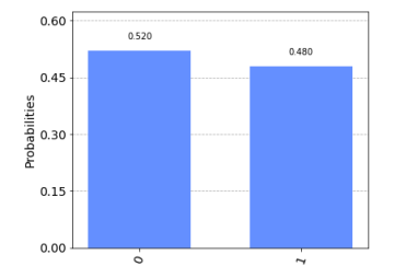
With this recipe, we will do 1,000 coin tosses in the blink of an eye and take a look at the results to see how good the coin is. Will this coin be a fair way to start, say, a game of baseball? Let’s see how that works.
The sample code for this recipe can be found here: https://github. com/ PacktPublishing/Quantum-Computing-in-Practice-with-Qiskitand-IBM-Quantum-Experience/blob/master/Chapter04/ch4_r2_coin_ tosses.py.
In this recipe, we will explore and expand on the shots job parameter. This parameter lets you control how many times you run the quantum job cycle – prepare, run, measure. So far, we have prepared our qubits in the $|0\rangle$ state, set the backend to a simulator, and then run one shot, which represents one full cycle.
In the IBM Quantum Experience composer examples, we ran our scores 1,024 times, which is the default. We discovered that the output turned statistical. In this recipe, we will play with a different number of shots to see how the outcomes statistically change.
Generally speaking, you want to increase the number of shots to improve statistical accuracy.
物理代写|量子计算代写Quantum computer代考|Implementing an upside-down coin toss
In this recipe, we will tweak our very first quantum program a little bit but still keep it relatively simple. An actual coin can be tossed starting with either heads or tails facing upward. Let’s do another quantum coin toss but with a different starting point, the coin facing tails up. In Dirac notation, we start with our qubit in $|1\rangle$ instead of in $|0\rangle$.
Getting ready
The sample code for this recipe can be found here: https://github. com/ PacktPublishing/Quantum-Computing-in-Practice-with-Qiskit-andIBM-Quantum-Experience/blob/master/Chapter04/ch4_r3_coin_toss_ tails.py.
Just like the previous recipe, this one is almost identical to the first coin toss recipe. Feel free to reuse what you have already created. The only real difference is that we add a new quantum gate, the $\mathbf{X}$ (or NOT) gate.
How to do it…
The following steps are to a large extent identical to the steps from the Quantum coin toss revisited recipe. There are, however, differences depending on the program you are creating, and what Qiskit” components you are using. I will describe these in detail.
Set up your code like the previous example and then add an $\mathrm{X}$ gate to flip the qubit:
- Import the required Qiskit” classes and methods:
from qiskit import QuantumCircuit, Aer, execute
from qiskit.visualization import plot_histogram
from IPython. core.display import display
Notice how we are not importing the QuantumRegister and
ClassicalRegister methods here like we did before. In this recipe, we will take
a look at a different way of creating your quantum circuit. - Create the quantum circuit with 1 qubit and 1 classical bit:
$q c=$ QuantumCircuit $(1,1)$
Here, we are implicitly letting the QuantumCircuit method create the quantum and classical registers in the background; we do not have to explicitly create them. We will refer to these registers by numbers and lists going forward. - Add the Hadamard gate, the $\mathrm{X}$ gate, and the measurement gates to the circuit:
qc.x $(0)$ qc.h $(0)$ qc.measure $(0,0)$
物理代写|量子计算代写Quantum computer代考|Tossing two coins simultaneously
So far, we have only played with one coin at a time, but there is nothing stopping us from adding more coins. In this recipe, we will add a coin to the simulation, and toss two coins simultaneously. We will do this by adding a second qubit, expanding the number of qubits – two of everything.
Getting ready
The sample code for this recipe can be found here: https://github . com/ PacktPublishing/Quantum-Computing-in-Practice-with-Qiskit-andIBM-Quantum-Experience/blob/master/Chapter04/ch4_r4_two_coin_ toss.py.
Set up your code like the previous example, but with a 2-qubit quantum circuit:
- Import the classes and methods that we need:
from qiskit import QuantumCircuit, Aer, execute
from qiskit.tools.visualization import plot_histogram
from IPython.core.display import display - Set up our quantum circuit with two qubits and two classical bits:
$q c=$ QuantumCircuit $(2,2)$ - Add the Hadamard gates and the measurement gates to the circuit:
qc $\cdot h([0,1])$
qc. measure $([0,1],[0,1])$
display (qc. draw (‘mpl’))
Note how we are now using lists to reference multiple qubits and multiple bits. For example, we apply the Hadamard gate to qubits 0 and 1 by using $[0,1]$ as input:
Figure $4.14$ – A 2 -qubit quantum coin toss circuit - Set the backend to our local simulator:
backend = Aer.get_backend (‘qasm_simulator’) - Run the job with one shot:
counts = execute (qc, backend, shots=1). result().
get_counts (qc)
Again, we are using streamlined code as we are only interested in the counts here.
量子计算代考
物理代写|量子计算代写Quantum computer代考|Getting some statistics – tossing many coins in a row
好的,到目前为止,我们一次只抛硬币,就像你在现实生活中所做的那样。
但量子计算的力量来自于在相同的初始条件下多次运行你的量子程序,让量子比特叠加发挥其量子力学优势,并统计总结大量运行。
使用这个食谱,我们将在眨眼之间进行 1,000 次硬币抛掷,看看结果,看看硬币有多好。这枚硬币会是开始棒球比赛的公平方式吗?让我们看看它是如何工作的。
这个配方的示例代码可以在这里找到:https://github。com/PacktPublishing/Quantum-Computing-in-Practice-with-Qiskitand-IBM-Quantum-Experience/blob/master/Chapter04/ch4_r2_coin_tosses.py。
在这个秘籍中,我们将探索和扩展镜头作业参数。此参数允许您控制运行量子作业周期的次数——准备、运行、测量。到目前为止,我们已经在|0⟩状态,将后端设置为模拟器,然后运行一个镜头,代表一个完整的周期。
在 IBM Quantum Experience 作曲家示例中,我们运行了 1,024 次得分,这是默认值。我们发现输出变成了统计数据。在这个秘籍中,我们将使用不同数量的投篮来观察结果在统计上是如何变化的。
一般来说,您希望增加拍摄次数以提高统计准确性。
物理代写|量子计算代写Quantum computer代考|Implementing an upside-down coin toss
在这个秘籍中,我们将稍微调整我们的第一个量子程序,但仍然保持相对简单。一个真正的硬币可以从正面或反面朝上开始投掷。让我们再掷一次量子硬币,但起点不同,硬币朝上。在狄拉克符号中,我们从我们的量子比特开始|1⟩而不是在|0⟩.
准备
可以在此处找到此配方的示例代码:https://github。com/PacktPublishing/Quantum-Computing-in-Practice-with-Qiskit-andIBM-Quantum-Experience/blob/master/Chapter04/ch4_r3_coin_toss_tails.py。
就像之前的食谱一样,这个几乎与第一个掷硬币的食谱相同。随意重用您已经创建的内容。唯一真正的区别是我们添加了一个新的量子门,X(或非)门。
怎么做……
以下步骤在很大程度上与重新审视量子硬币抛硬币的步骤相同。但是,根据您创建的程序以及您使用的 Qiskit 组件的不同,存在差异。我将详细描述这些。
像前面的例子一样设置你的代码,然后添加一个X翻转量子比特的门:
- 导入所需的 Qiskit” 类和方法:
from qiskit import QuantumCircuit, Aer,
从 qiskit.visualization 执行 import plot_histogram
from IPython。core.display import display
注意我们没有
像以前那样在这里导入 QuantumRegister 和 ClassicalRegister 方法。在这个秘籍中,我们将
看看创建量子电路的另一种方法。 - 创建具有 1 个量子位和 1 个经典位的量子电路:
qC=量子电路(1,1)
在这里,我们隐含地让 QuantumCircuit 方法在后台创建量子寄存器和经典寄存器;我们不必显式地创建它们。我们将通过数字和列表来引用这些寄存器。 - 添加 Hadamard 门,X门,以及电路的测量门:
qc.x(0)质量控制(0)质量控制测量(0,0)
物理代写|量子计算代写Quantum computer代考|Tossing two coins simultaneously
到目前为止,我们一次只玩一个硬币,但没有什么能阻止我们添加更多的硬币。在这个秘籍中,我们将在模拟中添加一枚硬币,并同时掷出两枚硬币。我们将通过添加第二个量子位来做到这一点,扩大量子位的数量——所有的两个。
准备好
这个食谱的示例代码可以在这里找到:https://github。com/PacktPublishing/Quantum-Computing-in-Practice-with-Qiskit-andIBM-Quantum-Experience/blob/master/Chapter04/ch4_r4_two_coin_toss.py。
像前面的示例一样设置您的代码,但使用 2-qubit 量子电路:
- 导入我们需要的类和方法:
from qiskit import QuantumCircuit, Aer, execute
from qiskit.tools.visualization import plot_histogram
from IPython.core.display import display - 用两个量子位和两个经典位建立我们的量子电路:
qC=量子电路(2,2) - 将 Hadamard 门和测量门添加到电路中:
qc⋅H([0,1])
质量控制。措施([0,1],[0,1])
display (qc.draw (‘mpl’))
注意我们现在如何使用列表来引用多个量子位和多个位。例如,我们通过使用将 Hadamard 门应用于 qubits 0 和 1[0,1]作为输入:
图4.14– 一个 2 量子比特的量子抛硬币电路 - 将后端设置为我们的本地模拟器:
backend = Aer.get_backend (‘qasm_simulator’) - 一次性运行作业:
counts = execute (qc, backend, shot=1)。结果()。
get_counts (qc)
同样,我们使用的是流线型代码,因为我们只对这里的计数感兴趣。

统计代写请认准statistics-lab™. statistics-lab™为您的留学生涯保驾护航。
金融工程代写
金融工程是使用数学技术来解决金融问题。金融工程使用计算机科学、统计学、经济学和应用数学领域的工具和知识来解决当前的金融问题,以及设计新的和创新的金融产品。
非参数统计代写
非参数统计指的是一种统计方法,其中不假设数据来自于由少数参数决定的规定模型;这种模型的例子包括正态分布模型和线性回归模型。
广义线性模型代考
广义线性模型(GLM)归属统计学领域,是一种应用灵活的线性回归模型。该模型允许因变量的偏差分布有除了正态分布之外的其它分布。
术语 广义线性模型(GLM)通常是指给定连续和/或分类预测因素的连续响应变量的常规线性回归模型。它包括多元线性回归,以及方差分析和方差分析(仅含固定效应)。
有限元方法代写
有限元方法(FEM)是一种流行的方法,用于数值解决工程和数学建模中出现的微分方程。典型的问题领域包括结构分析、传热、流体流动、质量运输和电磁势等传统领域。
有限元是一种通用的数值方法,用于解决两个或三个空间变量的偏微分方程(即一些边界值问题)。为了解决一个问题,有限元将一个大系统细分为更小、更简单的部分,称为有限元。这是通过在空间维度上的特定空间离散化来实现的,它是通过构建对象的网格来实现的:用于求解的数值域,它有有限数量的点。边界值问题的有限元方法表述最终导致一个代数方程组。该方法在域上对未知函数进行逼近。[1] 然后将模拟这些有限元的简单方程组合成一个更大的方程系统,以模拟整个问题。然后,有限元通过变化微积分使相关的误差函数最小化来逼近一个解决方案。
tatistics-lab作为专业的留学生服务机构,多年来已为美国、英国、加拿大、澳洲等留学热门地的学生提供专业的学术服务,包括但不限于Essay代写,Assignment代写,Dissertation代写,Report代写,小组作业代写,Proposal代写,Paper代写,Presentation代写,计算机作业代写,论文修改和润色,网课代做,exam代考等等。写作范围涵盖高中,本科,研究生等海外留学全阶段,辐射金融,经济学,会计学,审计学,管理学等全球99%专业科目。写作团队既有专业英语母语作者,也有海外名校硕博留学生,每位写作老师都拥有过硬的语言能力,专业的学科背景和学术写作经验。我们承诺100%原创,100%专业,100%准时,100%满意。
随机分析代写
随机微积分是数学的一个分支,对随机过程进行操作。它允许为随机过程的积分定义一个关于随机过程的一致的积分理论。这个领域是由日本数学家伊藤清在第二次世界大战期间创建并开始的。
时间序列分析代写
随机过程,是依赖于参数的一组随机变量的全体,参数通常是时间。 随机变量是随机现象的数量表现,其时间序列是一组按照时间发生先后顺序进行排列的数据点序列。通常一组时间序列的时间间隔为一恒定值(如1秒,5分钟,12小时,7天,1年),因此时间序列可以作为离散时间数据进行分析处理。研究时间序列数据的意义在于现实中,往往需要研究某个事物其随时间发展变化的规律。这就需要通过研究该事物过去发展的历史记录,以得到其自身发展的规律。
回归分析代写
多元回归分析渐进(Multiple Regression Analysis Asymptotics)属于计量经济学领域,主要是一种数学上的统计分析方法,可以分析复杂情况下各影响因素的数学关系,在自然科学、社会和经济学等多个领域内应用广泛。
MATLAB代写
MATLAB 是一种用于技术计算的高性能语言。它将计算、可视化和编程集成在一个易于使用的环境中,其中问题和解决方案以熟悉的数学符号表示。典型用途包括:数学和计算算法开发建模、仿真和原型制作数据分析、探索和可视化科学和工程图形应用程序开发,包括图形用户界面构建MATLAB 是一个交互式系统,其基本数据元素是一个不需要维度的数组。这使您可以解决许多技术计算问题,尤其是那些具有矩阵和向量公式的问题,而只需用 C 或 Fortran 等标量非交互式语言编写程序所需的时间的一小部分。MATLAB 名称代表矩阵实验室。MATLAB 最初的编写目的是提供对由 LINPACK 和 EISPACK 项目开发的矩阵软件的轻松访问,这两个项目共同代表了矩阵计算软件的最新技术。MATLAB 经过多年的发展,得到了许多用户的投入。在大学环境中,它是数学、工程和科学入门和高级课程的标准教学工具。在工业领域,MATLAB 是高效研究、开发和分析的首选工具。MATLAB 具有一系列称为工具箱的特定于应用程序的解决方案。对于大多数 MATLAB 用户来说非常重要,工具箱允许您学习和应用专业技术。工具箱是 MATLAB 函数(M 文件)的综合集合,可扩展 MATLAB 环境以解决特定类别的问题。可用工具箱的领域包括信号处理、控制系统、神经网络、模糊逻辑、小波、仿真等。