如果你也在 怎样代写主成分分析Principal Component Analysis这个学科遇到相关的难题,请随时右上角联系我们的24/7代写客服。
主成分分析(PCA)是计算主成分并使用它们对数据进行基础改变的过程,有时只使用前几个主成分,而忽略其余部分。
statistics-lab™ 为您的留学生涯保驾护航 在代写主成分分析Principal Component Analysis方面已经树立了自己的口碑, 保证靠谱, 高质且原创的统计Statistics代写服务。我们的专家在代写主成分分析Principal Component Analysis代写方面经验极为丰富,各种代写主成分分析Principal Component Analysis相关的作业也就用不着说。
我们提供的主成分分析Principal Component Analysis及其相关学科的代写,服务范围广, 其中包括但不限于:
- Statistical Inference 统计推断
- Statistical Computing 统计计算
- Advanced Probability Theory 高等概率论
- Advanced Mathematical Statistics 高等数理统计学
- (Generalized) Linear Models 广义线性模型
- Statistical Machine Learning 统计机器学习
- Longitudinal Data Analysis 纵向数据分析
- Foundations of Data Science 数据科学基础
统计代写|主成分分析代写Principal Component Analysis代考|Explained Variance
Finally, we introduce bounds for the explained variance $E V(X)$. Two results are obtained. The first is general and applicable to any basis $X$, not limited to sparse ones. The second is tailored to SPCArt.
Theorem 12 Let rank-r SVD of $A \in \mathbb{R}^{n \times p}$ be $U \Sigma V^{T}, \Sigma \in \mathbb{R}^{r \times r}$. Given $X \in \mathbb{R}^{p \times r}$, assume the $S V D$ of $X^{T} V$ to be $W D Q^{T}, D \in \mathbb{R}^{r \times r}, d_{\min }=\min {i} D{i i}$, then
$$
d_{\min }^{2} \cdot E V(V) \leq E V(X),
$$
and $E V(V)=\sum_{i} \Sigma_{i i^{\circ}}^{2}$
The theorem can be interpreted as follows. If $X$ is a basis that approximates the rotated PCA loadings well, then $d_{\min }$ will be close to one, and so the variance explained by $X$ is close to that explained by PCA. Note that the variance explained by PCA loadings is the largest value that is possible to be achieved by an orthonormal basis. Conversely, if $X$ deviates greatly from the rotated PCA loadings, then $d_{\min }$ tends to zero, so the variance explained by $X$ is not guaranteed to be large. Thus, the less the sparse loadings deviate from the rotated PCA loadings, the more variance they explain.
When SPCArt converges, i.e., $X_{i}=T_{\lambda}\left(Z_{i}\right) /\left|T_{\lambda}\left(Z_{i}\right)\right|_{2}$, where $Z=V R^{T}$, and $R=\operatorname{Polar}\left(X^{T} V\right)$ hold simultaneously, there is another estimation (mainly valid for $\mathrm{T}$-en).
Theorem 13 Let $C=Z^{T} X$, i.e., $C_{i j}=\cos \left(\theta\left(Z_{i}, X_{j}\right)\right)$, and let $\bar{C}$ be the diagonalremoved version. Assume $\forall i, \theta\left(Z_{i}, X_{i}\right)=\theta$ and $\sum_{j}^{r} C_{i j}^{2} \leq 1$, then
$$
\left(\cos ^{2}(\theta)-\sqrt{r-1} \sin (2 \theta)\right) \cdot E V(V) \leq E V(X) .
$$
When $\theta$ is sufficiently small,
$$
\left(\cos ^{2}(\theta)-O(\theta)\right) \cdot E V(V) \leq E V(X) .
$$
Since the sparse loadings are obtained by truncating small entries of the rotated PCA loadings, and $\theta$ is the deviation angle, the theorem implies that if the deviation
is small then the explained variance is close to that of $\mathrm{PCA}$, as $\cos ^{2}(\theta) \approx 1$. For example, if the truncated energy $|\bar{z}|_{2}^{2}=\sin ^{2}(\theta)$ is approximately $0.05$, then $95 \%$ $\mathrm{EV}$ of $\mathrm{PCA}$ loadings is guaranteed.
The assumptions $\theta\left(Z_{i}, X_{i}\right)=\theta$ and $\sum_{j}^{r} C_{i j}^{2} \leq 1, \forall i$, are broadly satisfied by T-en using small $\lambda$. Uniform deviation $\theta\left(Z_{i}, X_{i}\right)=\theta \forall i$ can be achieved by T-en, as indicated by Proposition 11. $\sum_{j}^{r} C_{i j}^{2} \leq 1$ means the sum of projected length is less than 1 when $Z_{i}$ is projected onto each $X_{j}$. It is satisfied if $X$ is exactly orthogonal, whereas it is likely satisfied if $X$ is nearly orthogonal (note $Z_{i}$ may not lie in the subspace spanned by $X$ ), which can be achieved by setting small $\lambda$ according to Proposition 6. In this case, about $(1-\lambda) E V(V)$ is guaranteed.
In practice, we prefer CPEV [21] to EV. CPEV measures the variance explained by subspace rather than basis. Since it is also the projected length of $A$ onto the subspace spanned by $X$, the higher CPEV, the better $X$ represents the data. If $X$ is not an orthogonal basis, EV may overestimate or underestimate the variance. However, if $X$ is nearly orthogonal, the difference is small, and it is nearly proportional to CPEV.
统计代写|主成分分析代写Principal Component Analysis代考|A Unified View to Some Prior Work
A series of methods: PCA [10], SCoTLASS [11], SPCA [29], GPower [13], $\mathrm{rSVD}[21]$, TPower [25], SPC [24], and SPCArt, although proposed independently and formulated in various forms, can be derived from the common source of Theorem 1, the Eckart-Young Theorem. Most of them can be seen as the problems of matrix approximation (1), with different sparsity penalties. Most of them have two matrix variables, and the solutions of them can usually be obtained by an alternating scheme: fixing one and solving the other. Similar to SPCArt, the two subproblems are a sparsity penalized/constrained regression problem and a Procrustes problem.
PCA [10]. Since $Y^{}=A X^{}$, substituting $Y=A X$ into (1) and optimizing $X$, the problem is equivalent to
$$
\max {X} \operatorname{tr}\left(X^{T} A^{T} A X\right), \text { s.t. } X^{T} X=I . $$ By the Ky Fan theorem [7], $X^{}=V{1: r} R, \forall R^{T} R=I$. If $A$ is a mean-removed data matrix, the special solution $X^{}=V_{1 r}$ contains exactly the $r$ loadings obtained by PCA.
SCoTLASS [11]. Constraining $X$ to be sparse in (19), we get SCotLASS
$$
\max {X} \operatorname{tr}\left(X^{T} A^{T} A X\right), \text { s.t. } X^{T} X=I, \forall i,\left|X{i}\right|_{1} \leq \lambda
$$
Unfortunately, this problem is not easy to solve.
统计代写|主成分分析代写Principal Component Analysis代考|Principal Component Analysis (PCA) Based
Principal component analysis (PCA) $[10,12,27]$ is an orthogonal basis transformation with the advantage that the first few principal components preserve most of the variance of the data set. This method [27], initially, calculates the covariance matrix of the given data set, and then finds the eigenvalues and eigenvectors of this matrix. Next it selects a few eigenvectors whose eigenvalues are more to form the transformation matrix to reduce the dimensions of the data set.
Suppose, there are $D$ number of band images. So, a pixel has $D$ number of different responses over different wavelengths. As a consequences, a pixel may be treated as a pattern of $D$ attributes. The main target is to reduce the dimensionality from $D$ to $d(d \ll D)$ of hyperspectral image pixel.
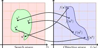
Let, there be a set of pattern $x_{i}$, where $x_{i} \in \mathfrak{R}^{D}, i=1,2, \ldots, N$. Assume that the data are centered, i.e., $x_{i} \Longleftarrow x_{i}-E\left{x_{i}\right}$. Conventional PCA formulates the eigenvalue problem by
$$
\lambda V=\Sigma_{x} V
$$
where $\lambda$ is eigenvalue, $V$ is eigenvector, $\Sigma_{x}$ is the corresponding covariance matrix over data set $x$ which is calculated by the following equation
$$
\Sigma_{x}=\frac{1}{N} \sum_{i=1}^{N} x_{i} x_{i}^{T}
$$
The projection on the eigenvector $V^{k}$ is calculated as
$$
x_{p c}^{k}=V^{k} . x .
$$
The principal component based transformation is defined as
$$
y_{i}=W^{T} x_{i}
$$
where $W$ is the matrix of first $d$ normalized eigenvectors of highest eigenvalues of the image covariance matrix $\Sigma_{x} . T$ denotes the transpose operation.
Here, a pattern $x_{i}$ from original $D$-dimensional space is transformed into $y_{i}$, a pattern in reduced $d$-dimensional space by choosing only the first $d$ components (eigenvectors of highest $d$ eigenvalues).
The transformed data set has two main properties which are significant to the application here. The variance in the original data set has been rearranged and reordered so that first few components contain almost all of the variance in the original data, and the components in the new feature space are uncorrelated in nature [20].
主成分分析代考
统计代写|主成分分析代写Principal Component Analysis代考|Explained Variance
最后,我们引入解释方差的界限和在(X). 得到两个结果。第一个是通用的,适用于任何基础X,不限于稀疏的。第二个是为 SPCArt 量身定做的。
定理 12 令 rank-r SVD 为一个∈Rn×p是在Σ在吨,Σ∈Rr×r. 给定X∈Rp×r,假设小号在D的X吨在为 $WDQ^{T}, D \in \mathbb{R}^{r \times r}, d_{\min }=\min {i} D {ii},吨H和nd分钟2⋅和在(在)≤和在(X),一个ndEV(V)=\sum_{i} \Sigma_{ii^{\circ}}^{2}吨H和吨H和○r和米C一个nb和一世n吨和rpr和吨和d一个sF○ll○在s.我FX一世s一个b一个s一世s吨H一个吨一个ppr○X一世米一个吨和s吨H和r○吨一个吨和d磷C一个l○一个d一世nGs在和ll,吨H和nd_{\分钟}在一世llb和Cl○s和吨○○n和,一个nds○吨H和在一个r一世一个nC和和Xpl一个一世n和db是X一世sCl○s和吨○吨H一个吨和Xpl一个一世n和db是磷C一个.ñ○吨和吨H一个吨吨H和在一个r一世一个nC和和Xpl一个一世n和db是磷C一个l○一个d一世nGs一世s吨H和l一个rG和s吨在一个l在和吨H一个吨一世sp○ss一世bl和吨○b和一个CH一世和在和db是一个n○r吨H○n○r米一个lb一个s一世s.C○n在和rs和l是,一世FXd和在一世一个吨和sGr和一个吨l是Fr○米吨H和r○吨一个吨和d磷C一个l○一个d一世nGs,吨H和nd_{\分钟}吨和nds吨○和和r○,s○吨H和在一个r一世一个nC和和Xpl一个一世n和db是X$ 不保证很大。因此,稀疏载荷与旋转 PCA 载荷的偏差越小,它们解释的方差就越多。
当 SPCArt 收敛时,即X一世=吨λ(从一世)/|吨λ(从一世)|2, 在哪里从=在R吨, 和R=极性(X吨在)同时保持,还有另一个估计(主要适用于吨-在)。
定理 13 让C=从吨X, IE,C一世j=因(θ(从一世,Xj)), 然后让C¯是对角线删除的版本。认为∀一世,θ(从一世,X一世)=θ和∑jrC一世j2≤1, 然后
(因2(θ)−r−1罪(2θ))⋅和在(在)≤和在(X).
什么时候θ足够小,
(因2(θ)−○(θ))⋅和在(在)≤和在(X).
由于稀疏载荷是通过截断旋转 PCA 载荷的小条目获得的,并且θ是偏差角,该定理意味着如果偏差
小,则解释的方差接近磷C一个, 作为因2(θ)≈1. 例如,如果截断能量|和¯|22=罪2(θ)大约是0.05, 然后95% 和在的磷C一个保证负载。
假设θ(从一世,X一世)=θ和∑jrC一世j2≤1,∀一世, 被 T-en 广泛满足λ. 均匀偏差θ(从一世,X一世)=θ∀一世可以通过 T-en 来实现,如命题 11 所示。∑jrC一世j2≤1表示投影长度之和小于 1 时从一世被投影到每个Xj. 如果满足X是完全正交的,而如果X几乎是正交的(注意从一世不能位于跨越的子空间中X),这可以通过设置小来实现λ根据命题 6。在这种情况下,大约(1−λ)和在(在)得到保证。
在实践中,我们更喜欢 CPEV [21] 而不是 EV。CPEV 测量由子空间而不是基解释的方差。因为它也是投影长度一个到跨越的子空间X, CPEV 越高越好X表示数据。如果X不是正交基,EV 可能高估或低估方差。然而,如果X几乎正交,差异很小,并且几乎与 CPEV 成正比。
统计代写|主成分分析代写Principal Component Analysis代考|A Unified View to Some Prior Work
一系列方法:PCA [10]、SCoTLASS [11]、SPCA [29]、GPower [13]、r小号在D[21]、TPower [25]、SPC [24] 和 SPCArt,虽然是独立提出并以各种形式表述的,但可以从定理 1 的共同来源,即 Eckart-Young 定理推导出来。它们中的大多数可以看作是矩阵近似(1)的问题,具有不同的稀疏惩罚。它们中的大多数有两个矩阵变量,它们的解通常可以通过交替方案获得:固定一个,求解另一个。与 SPCArt 类似,这两个子问题是稀疏惩罚/约束回归问题和 Procrustes 问题。
主成分分析 [10]。自从是=一个X, 代入是=一个X进入(1)并优化X, 问题等价于
最大限度Xtr(X吨一个吨一个X), 英石 X吨X=我.由 Ky Fan 定理 [7],X=在1:rR,∀R吨R=我. 如果一个是一个均值去除的数据矩阵,特殊解X=在1r正好包含rPCA 获得的载荷。
斯科特拉斯 [11]。约束X为了在 (19) 中稀疏,我们得到 SCotLASS
最大限度Xtr(X吨一个吨一个X), 英石 X吨X=我,∀一世,|X一世|1≤λ
不幸的是,这个问题并不容易解决。
统计代写|主成分分析代写Principal Component Analysis代考|Principal Component Analysis (PCA) Based
主成分分析(PCA)[10,12,27]是正交基变换,其优点是前几个主成分保留了数据集的大部分方差。该方法 [27] 最初计算给定数据集的协方差矩阵,然后找到该矩阵的特征值和特征向量。接下来选取特征值较多的几个特征向量组成变换矩阵,对数据集进行降维。
假设,有D带图像的数量。所以,一个像素有D在不同波长上的不同响应的数量。因此,一个像素可以被视为一种模式D属性。主要目标是从D至d(d≪D)的高光谱图像像素。
让,有一组模式X一世, 在哪里X一世∈RD,一世=1,2,…,ñ. 假设数据居中,即x_{i} \Longleftarrow x_{i}-E\left{x_{i}\right}x_{i} \Longleftarrow x_{i}-E\left{x_{i}\right}. 传统的 PCA 通过以下方式制定特征值问题
λ在=ΣX在
在哪里λ是特征值,在是特征向量,ΣX是数据集上对应的协方差矩阵X通过以下等式计算
ΣX=1ñ∑一世=1ñX一世X一世吨
特征向量上的投影在ķ计算为
XpCķ=在ķ.X.
基于主成分的变换定义为
是一世=在吨X一世
在哪里在是第一个矩阵d图像协方差矩阵的最高特征值的归一化特征向量ΣX.吨表示转置操作。
在这里,一个图案X一世从原始D维空间被转化为是一世,减少的模式d- 仅选择第一个维度空间d分量(最高的特征向量d特征值)。
转换后的数据集有两个对这里的应用程序很重要的主要属性。原始数据集中的方差已被重新排列和重新排序,以便前几个分量包含原始数据中几乎所有的方差,而新特征空间中的分量本质上是不相关的 [20]。

统计代写请认准statistics-lab™. statistics-lab™为您的留学生涯保驾护航。
金融工程代写
金融工程是使用数学技术来解决金融问题。金融工程使用计算机科学、统计学、经济学和应用数学领域的工具和知识来解决当前的金融问题,以及设计新的和创新的金融产品。
非参数统计代写
非参数统计指的是一种统计方法,其中不假设数据来自于由少数参数决定的规定模型;这种模型的例子包括正态分布模型和线性回归模型。
广义线性模型代考
广义线性模型(GLM)归属统计学领域,是一种应用灵活的线性回归模型。该模型允许因变量的偏差分布有除了正态分布之外的其它分布。
术语 广义线性模型(GLM)通常是指给定连续和/或分类预测因素的连续响应变量的常规线性回归模型。它包括多元线性回归,以及方差分析和方差分析(仅含固定效应)。
有限元方法代写
有限元方法(FEM)是一种流行的方法,用于数值解决工程和数学建模中出现的微分方程。典型的问题领域包括结构分析、传热、流体流动、质量运输和电磁势等传统领域。
有限元是一种通用的数值方法,用于解决两个或三个空间变量的偏微分方程(即一些边界值问题)。为了解决一个问题,有限元将一个大系统细分为更小、更简单的部分,称为有限元。这是通过在空间维度上的特定空间离散化来实现的,它是通过构建对象的网格来实现的:用于求解的数值域,它有有限数量的点。边界值问题的有限元方法表述最终导致一个代数方程组。该方法在域上对未知函数进行逼近。[1] 然后将模拟这些有限元的简单方程组合成一个更大的方程系统,以模拟整个问题。然后,有限元通过变化微积分使相关的误差函数最小化来逼近一个解决方案。
tatistics-lab作为专业的留学生服务机构,多年来已为美国、英国、加拿大、澳洲等留学热门地的学生提供专业的学术服务,包括但不限于Essay代写,Assignment代写,Dissertation代写,Report代写,小组作业代写,Proposal代写,Paper代写,Presentation代写,计算机作业代写,论文修改和润色,网课代做,exam代考等等。写作范围涵盖高中,本科,研究生等海外留学全阶段,辐射金融,经济学,会计学,审计学,管理学等全球99%专业科目。写作团队既有专业英语母语作者,也有海外名校硕博留学生,每位写作老师都拥有过硬的语言能力,专业的学科背景和学术写作经验。我们承诺100%原创,100%专业,100%准时,100%满意。
随机分析代写
随机微积分是数学的一个分支,对随机过程进行操作。它允许为随机过程的积分定义一个关于随机过程的一致的积分理论。这个领域是由日本数学家伊藤清在第二次世界大战期间创建并开始的。
时间序列分析代写
随机过程,是依赖于参数的一组随机变量的全体,参数通常是时间。 随机变量是随机现象的数量表现,其时间序列是一组按照时间发生先后顺序进行排列的数据点序列。通常一组时间序列的时间间隔为一恒定值(如1秒,5分钟,12小时,7天,1年),因此时间序列可以作为离散时间数据进行分析处理。研究时间序列数据的意义在于现实中,往往需要研究某个事物其随时间发展变化的规律。这就需要通过研究该事物过去发展的历史记录,以得到其自身发展的规律。
回归分析代写
多元回归分析渐进(Multiple Regression Analysis Asymptotics)属于计量经济学领域,主要是一种数学上的统计分析方法,可以分析复杂情况下各影响因素的数学关系,在自然科学、社会和经济学等多个领域内应用广泛。
MATLAB代写
MATLAB 是一种用于技术计算的高性能语言。它将计算、可视化和编程集成在一个易于使用的环境中,其中问题和解决方案以熟悉的数学符号表示。典型用途包括:数学和计算算法开发建模、仿真和原型制作数据分析、探索和可视化科学和工程图形应用程序开发,包括图形用户界面构建MATLAB 是一个交互式系统,其基本数据元素是一个不需要维度的数组。这使您可以解决许多技术计算问题,尤其是那些具有矩阵和向量公式的问题,而只需用 C 或 Fortran 等标量非交互式语言编写程序所需的时间的一小部分。MATLAB 名称代表矩阵实验室。MATLAB 最初的编写目的是提供对由 LINPACK 和 EISPACK 项目开发的矩阵软件的轻松访问,这两个项目共同代表了矩阵计算软件的最新技术。MATLAB 经过多年的发展,得到了许多用户的投入。在大学环境中,它是数学、工程和科学入门和高级课程的标准教学工具。在工业领域,MATLAB 是高效研究、开发和分析的首选工具。MATLAB 具有一系列称为工具箱的特定于应用程序的解决方案。对于大多数 MATLAB 用户来说非常重要,工具箱允许您学习和应用专业技术。工具箱是 MATLAB 函数(M 文件)的综合集合,可扩展 MATLAB 环境以解决特定类别的问题。可用工具箱的领域包括信号处理、控制系统、神经网络、模糊逻辑、小波、仿真等。