如果你也在 怎样代写商业分析Statistical Modelling for Business这个学科遇到相关的难题,请随时右上角联系我们的24/7代写客服。
商业分析就是利用数据分析和统计的方法,来分析企业之前的商业表现,从而通过分析结果来对未来的商业战略进行预测和指导 。
statistics-lab™ 为您的留学生涯保驾护航 在代写商业分析Statistical Modelling for Business方面已经树立了自己的口碑, 保证靠谱, 高质且原创的统计Statistics代写服务。我们的专家在代写商业分析Statistical Modelling for Business方面经验极为丰富,各种代写商业分析Statistical Modelling for Business相关的作业也就用不着说。
我们提供的商业分析Statistical Modelling for Business及其相关学科的代写,服务范围广, 其中包括但不限于:
- Statistical Inference 统计推断
- Statistical Computing 统计计算
- Advanced Probability Theory 高等楖率论
- Advanced Mathematical Statistics 高等数理统计学
- (Generalized) Linear Models 广义线性模型
- Statistical Machine Learning 统计机器学习
- Longitudinal Data Analysis 纵向数据分析
- Foundations of Data Science 数据科学基础
统计代写|商业分析作业代写Statistical Modelling for Business代考|Studying Pizza Preferences by Using
Part 1: Studying Pizza Preferences by Using a Frequency Distribution Unfortunately, the raw data in Table $2.1$ do not reveal much useful information about the pattern of pizza preferences. In order to summarize the data in a more useful way, we can construct a frequency distribution. To do this we simply count the number of times each of the six pizza restaurants appears in Table 2.1. We find that Bruno’s appears 8 times, Domino’s appears 2 times, Little Caesars appears 9 times, Papa John’s appears 19 times, Pizza Hut appears 4 times, and Will’s Uptown Pizza appears 8 times. The frequency distribution for the pizza preferences is given in Table $2.2$ on the next page-a list of each of the six restaurants along with their corresponding counts (or frequencies). The frequency distribution shows us how the preferences are distributed among the six restaurants. The purpose of the frequency
distribution is to make the data easier to understand. Certainly, looking at the frequency distribution in Table $2.2$ is more informative than looking at the raw data in Table 2.1. We see that Papa John’s is the most popular restaurant, and that Papa John’s is roughly twice as popular as each of the next three runners-up-Bruno’s, Little Caesars, and Will’s. Finally, Pizza Hut and Domino’s are the least preferred restaurants.
When we wish to summarize the proportion (or fraction) of items in each class, we employ the relative frequency for each class. If the data set consists of $n$ observations, we define the relative frequency of a class as follows:
Relative frequency of a class $=\frac{\text { frequency of the class }}{h}$
This quantity is simply the fraction of items in the class. Further, we can obtain the percent frequency of a class by multiplying the relative frequency by 100 .
Table $2.3$ gives a relative frequency distribution and a percent frequency distribution of the pizza preference data. A relative frequency distribution is a table that lists the relative frequency for each class, and a percent frequency distribution lists the percent frequency for each class. Looking at Table $2.3$, we see that the relative frequency for Bruno’s pizza is $8 / 50=.16$ and that (from the percent frequency distribution) $16 \%$ of the sampled students preferred Bruno’s pizza. Similarly, the relative frequency for Papa John’s pizza is $19 / 50=$ $.38$ and $38 \%$ of the sampled students preferred Papa John’s pizza. Finally, the sum of the relative frequencies in the relative frequency distribution equals $1.0$, and the sum of the percent frequencies in the percent frequency distribution equals $100 \%$. These facts are true for all relative frequency and percent frequency distributions.
统计代写|商业分析作业代写Statistical Modelling for Business代考|Studying Pizza Preferences
Part 2: Studying Pizza Preferences by Using Bar Charts and Pie Charts A bar chart is a graphic that depicts a frequency, relative frequency, or percent frequency distribution. For example, Figure $2.1$ gives an Excel bar chart of the pizza preference data. On the horizontal axis we have placed a label for each class (restaurant), while the vertical axis measures frequencies. To construct the bar chart, Excel draws a bar (of fixed width) corresponding to each class label.
Each bar is drawn so that its height equals the frequency corresponding to its label. Because the height of each bar is a frequency, we refer to Figure $2.1$ as a frequency bar chart. Notice that there are gaps between the bars. When data are qualitative, the bars should always be separated by gaps in order to indicate that each class is separate from the others. The bar chart in Figure $2.1$ clearly illustrates that, for example, Papa Juhits pizca is preferred by more sampled students than any other restaurant and Domino’s pizza is least preferred by the sampled students.
If desired, the har heights can represent relative frequencies or percent frequencies For instance, Figure $2.2$ is a Minitab percent bar chart for the pizza preference data. Here the heights of the bars are the percentages given in the percent frequency distribution of Table 2.3. Lastly, the bars in Figures $2.1$ and $2.2$ have been positioned vertically. Because of this, these bar charts are called vertical bar charts. However, sometimes bar charts are constructed with horizontal bars and are called horizontal bar charts.
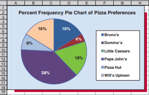
A pie chart is another graphic that can be used to depict a frequency distribution. When constructing a pie chart, we first draw a circle to represent the entire data set. We then divide the circle into sectors or “pie slices” based on the relative frequencies of the classes. For example, remembering that a circle consists of 360 degrees, Bruno’s Pizza (which has relative frequency .16) is assigned a pie slice that consists of $.16(360)=57.6$ degrees. Similarly, Papa John’s Pizza (with relative frequency .38) is assigned a pie slice having. $.38(360)=$ $136.8$ degrees. The resulting pie chart (constructed using Excel) is shown in Figure $2.3$ on the next page. Here we have labeled the pie slices using the percent frequencies. The pie slices can also be labeled using frequencies or relative frequencies.
统计代写|商业分析作业代写Statistical Modelling for Business代考|The Pareto chart (Optional)
Pareto charts are used to help identify important quality problems and opportunities for process improvement. By using these charts we can prioritize problem-solving activities. The Pareto chart is named for Vilfredo Pareto (1848-1923), an Italian economist. Pareto suggested that, in many economies, most of the wealth is held by a small minority of the population. It has been found that the “Pareto principle” often applies to defects. That is, only a few defect types account for most of a product’s quality problems.
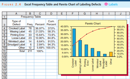
To illustrate the use of Pareto charts, suppose that a jelly producer wishes to evaluate the labels being placed on 16-ounce jars of grape jelly. Every day for two weeks, all defective labels found on inspection are classified by type of defect. If a label has more than one defect, the type of defect that is most noticeable is recorded. The Excel output in Figure $2.4$ presents the frequencies and percentages of the types of defects observed over the two-week period.
In general, the first step in setting up a Pareto chart summarizing data concerning types of defects (or categories) is to construct a frequency table like the one in Figure 2.4. Defects or categories should be listed at the left of the table in decreasing order by frequenciesthe defect with the highest frequency will be at the top of the table, the defect with the second-highest frequency below the first, and so forth. If an “other” category is employed, it should be placed at the bottom of the table. The “other” category should not make up 50 percent or more of the total of the frequencies, and the frequency for the “other” category should not exceed the frequency for the defect at the top of the table. If the frequency for the “other” category is too high, data should be collected so that the “other” category can be broken down into new categories. Once the frequency and the percentage for each category are determined, a cumulative percentage for each category is computed. As illustrated in Figure $2.4$, the cumulative percentage for a particular category is the sum of the percentages corresponding to the particular eategory and the categories that are above that category in the table.
金融中的随机方法代写
统计代写|商业分析作业代写Statistical Modelling for Business代考|Studying Pizza Preferences by Using
第 1 部分:使用频率分布研究比萨偏好 不幸的是,表中的原始数据2.1不要透露太多关于披萨偏好模式的有用信息。为了以更有用的方式汇总数据,我们可以构造频率分布。为此,我们只需计算表 2.1 中六家比萨餐厅中的每家出现的次数。我们发现 Bruno’s 出现了 8 次,Domino’s 出现了 2 次,Little Caesars 出现了 9 次,Papa John’s 出现了 19 次,Pizza Hut 出现了 4 次,Will’s Uptown Pizza 出现了 8 次。披萨偏好的频率分布在表中给出2.2在下一页上 – 六家餐厅中每家的列表及其相应的计数(或频率)。频率分布向我们展示了偏好在六家餐厅之间的分布情况。频率的目的
分布是为了让数据更容易理解。当然,看看表中的频率分布2.2比查看表 2.1 中的原始数据提供更多信息。我们看到 Papa John’s 是最受欢迎的餐厅,而 Papa John’s 的受欢迎程度大约是接下来三个亚军 Bruno’s、Little Caesars 和 Will’s 的两倍。最后,必胜客和达美乐是最不受欢迎的餐厅。
当我们希望总结每个类别中项目的比例(或分数)时,我们使用每个类别的相对频率。如果数据集由n观察,我们定义一个类的相对频率如下:
一个类的相对频率= 上课频率 H
这个数量只是类中项目的分数。此外,我们可以通过将相对频率乘以 100 来获得类的百分比频率。
桌子2.3给出比萨偏好数据的相对频率分布和百分比频率分布. 相对频率分布是列出每个类别的相对频率的表格,百分比频率分布列出每个类别的百分比频率。看表2.3,我们看到布鲁诺披萨的相对频率是8/50=.16和那个(从百分比频率分布)16%的抽样学生更喜欢布鲁诺的披萨。同样,棒约翰披萨的相对频率是19/50= .38和38%的抽样学生更喜欢 Papa John 的披萨。最后,相对频率分布中的相对频率之和等于1.0,并且百分比频率分布中的百分比频率之和等于100%. 这些事实适用于所有相对频率和百分比频率分布。
统计代写|商业分析作业代写Statistical Modelling for Business代考|Studying Pizza Preferences
第 2 部分:使用条形图和饼图研究比萨偏好 条形图是描述频率、相对频率或百分比频率分布的图形。例如,图2.1给出披萨偏好数据的 Excel 条形图. 在水平轴上,我们为每个类别(餐厅)放置了一个标签,而垂直轴测量频率。为了构建条形图,Excel 会绘制一个与每个类标签相对应的条形(固定宽度)。
绘制每个条形使其高度等于其标签对应的频率。因为每个条的高度是一个频率,我们参考图2.1作为频率条形图。请注意,条形之间存在间隙。当数据是定性的时,条形应始终由间隙隔开,以表明每个类与其他类是分开的。图中的条形图2.1清楚地表明,例如,Papa Juhits pizca 比任何其他餐厅更受抽样学生的青睐,而 Domino 的比萨饼是抽样学生最不喜欢的。
如果需要,har 高度可以表示相对频率或百分比频率。例如,图2.2是比萨偏好数据的 Minitab 百分比条形图。这里的条形高度是表 2.3 的百分比频率分布中给出的百分比。最后,图中的条形图2.1和2.2已垂直放置。因此,这些条形图被称为垂直条形图。但是,有时条形图由水平条构成,称为水平条形图。
饼图是另一种可用于描述频率分布的图形。在构建饼图时,我们首先画一个圆圈来表示整个数据集。然后,我们根据类的相对频率将圆圈分成扇区或“饼片”。例如,记住一个圆由 360 度组成,Bruno’s Pizza(相对频率为 0.16)被分配一个饼片,该饼片由.16(360)=57.6度。类似地,Papa John’s Pizza(相对频率为 0.38)被分配了一个饼片。.38(360)= 136.8度。生成的饼图(使用 Excel 构建)如图2.3在下一页。在这里,我们使用百分比频率标记了饼图。饼图切片也可以使用频率或相对频率来标记。
统计代写|商业分析作业代写Statistical Modelling for Business代考|The Pareto chart (Optional)
帕累托图用于帮助识别重要的质量问题和过程改进的机会。通过使用这些图表,我们可以优先考虑解决问题的活动。Pareto 图以意大利经济学家 Vilfredo Pareto (1848-1923) 命名。帕累托建议,在许多经济体中,大部分财富由少数人口持有。已经发现,“帕累托原理”通常适用于缺陷。也就是说,只有少数缺陷类型可以解决大部分产品的质量问题。
为了说明帕累托图的使用,假设果冻生产商希望评估放置在 16 盎司罐装葡萄果冻上的标签。两周内每天都会对检查中发现的所有缺陷标签按缺陷类型进行分类。如果标签有多个缺陷,则记录最明显的缺陷类型。图中的 Excel 输出2.4显示了在两周内观察到的缺陷类型的频率和百分比。
一般而言,建立帕累托图总结有关缺陷类型(或类别)的数据的第一步是构建一个如图 2.4 中所示的频率表。缺陷或类别应按频率降序排列在表的左侧,频率最高的缺陷将位于表的顶部,频率第二高的缺陷位于第一个之下,依此类推。如果使用“其他”类别,则应将其放在表格底部。“其他”类别不应占总频率的 50% 或更多,“其他”类别的频率不应超过表顶部缺陷的频率。如果“其他”类别的频率太高,应收集数据,以便将“其他”类别分解为新类别。一旦确定了每个类别的频率和百分比,就会计算每个类别的累积百分比。如图所示2.4,特定类别的累积百分比是对应于特定类别的百分比和表中高于该类别的类别的总和。

统计代写请认准statistics-lab™. statistics-lab™为您的留学生涯保驾护航。统计代写|python代写代考
随机过程代考
在概率论概念中,随机过程是随机变量的集合。 若一随机系统的样本点是随机函数,则称此函数为样本函数,这一随机系统全部样本函数的集合是一个随机过程。 实际应用中,样本函数的一般定义在时间域或者空间域。 随机过程的实例如股票和汇率的波动、语音信号、视频信号、体温的变化,随机运动如布朗运动、随机徘徊等等。
贝叶斯方法代考
贝叶斯统计概念及数据分析表示使用概率陈述回答有关未知参数的研究问题以及统计范式。后验分布包括关于参数的先验分布,和基于观测数据提供关于参数的信息似然模型。根据选择的先验分布和似然模型,后验分布可以解析或近似,例如,马尔科夫链蒙特卡罗 (MCMC) 方法之一。贝叶斯统计概念及数据分析使用后验分布来形成模型参数的各种摘要,包括点估计,如后验平均值、中位数、百分位数和称为可信区间的区间估计。此外,所有关于模型参数的统计检验都可以表示为基于估计后验分布的概率报表。
广义线性模型代考
广义线性模型(GLM)归属统计学领域,是一种应用灵活的线性回归模型。该模型允许因变量的偏差分布有除了正态分布之外的其它分布。
statistics-lab作为专业的留学生服务机构,多年来已为美国、英国、加拿大、澳洲等留学热门地的学生提供专业的学术服务,包括但不限于Essay代写,Assignment代写,Dissertation代写,Report代写,小组作业代写,Proposal代写,Paper代写,Presentation代写,计算机作业代写,论文修改和润色,网课代做,exam代考等等。写作范围涵盖高中,本科,研究生等海外留学全阶段,辐射金融,经济学,会计学,审计学,管理学等全球99%专业科目。写作团队既有专业英语母语作者,也有海外名校硕博留学生,每位写作老师都拥有过硬的语言能力,专业的学科背景和学术写作经验。我们承诺100%原创,100%专业,100%准时,100%满意。
机器学习代写
随着AI的大潮到来,Machine Learning逐渐成为一个新的学习热点。同时与传统CS相比,Machine Learning在其他领域也有着广泛的应用,因此这门学科成为不仅折磨CS专业同学的“小恶魔”,也是折磨生物、化学、统计等其他学科留学生的“大魔王”。学习Machine learning的一大绊脚石在于使用语言众多,跨学科范围广,所以学习起来尤其困难。但是不管你在学习Machine Learning时遇到任何难题,StudyGate专业导师团队都能为你轻松解决。
多元统计分析代考
基础数据: $N$ 个样本, $P$ 个变量数的单样本,组成的横列的数据表
变量定性: 分类和顺序;变量定量:数值
数学公式的角度分为: 因变量与自变量
时间序列分析代写
随机过程,是依赖于参数的一组随机变量的全体,参数通常是时间。 随机变量是随机现象的数量表现,其时间序列是一组按照时间发生先后顺序进行排列的数据点序列。通常一组时间序列的时间间隔为一恒定值(如1秒,5分钟,12小时,7天,1年),因此时间序列可以作为离散时间数据进行分析处理。研究时间序列数据的意义在于现实中,往往需要研究某个事物其随时间发展变化的规律。这就需要通过研究该事物过去发展的历史记录,以得到其自身发展的规律。
回归分析代写
多元回归分析渐进(Multiple Regression Analysis Asymptotics)属于计量经济学领域,主要是一种数学上的统计分析方法,可以分析复杂情况下各影响因素的数学关系,在自然科学、社会和经济学等多个领域内应用广泛。
MATLAB代写
MATLAB 是一种用于技术计算的高性能语言。它将计算、可视化和编程集成在一个易于使用的环境中,其中问题和解决方案以熟悉的数学符号表示。典型用途包括:数学和计算算法开发建模、仿真和原型制作数据分析、探索和可视化科学和工程图形应用程序开发,包括图形用户界面构建MATLAB 是一个交互式系统,其基本数据元素是一个不需要维度的数组。这使您可以解决许多技术计算问题,尤其是那些具有矩阵和向量公式的问题,而只需用 C 或 Fortran 等标量非交互式语言编写程序所需的时间的一小部分。MATLAB 名称代表矩阵实验室。MATLAB 最初的编写目的是提供对由 LINPACK 和 EISPACK 项目开发的矩阵软件的轻松访问,这两个项目共同代表了矩阵计算软件的最新技术。MATLAB 经过多年的发展,得到了许多用户的投入。在大学环境中,它是数学、工程和科学入门和高级课程的标准教学工具。在工业领域,MATLAB 是高效研究、开发和分析的首选工具。MATLAB 具有一系列称为工具箱的特定于应用程序的解决方案。对于大多数 MATLAB 用户来说非常重要,工具箱允许您学习和应用专业技术。工具箱是 MATLAB 函数(M 文件)的综合集合,可扩展 MATLAB 环境以解决特定类别的问题。可用工具箱的领域包括信号处理、控制系统、神经网络、模糊逻辑、小波、仿真等。