如果你也在 怎样代写多元统计分析Multivariate Statistical Analysis这个学科遇到相关的难题,请随时右上角联系我们的24/7代写客服。
多变量统计分析被认为是评估地球化学异常与任何单独变量和变量之间相互影响的意义的有用工具。
statistics-lab™ 为您的留学生涯保驾护航 在代写多元统计分析Multivariate Statistical Analysis方面已经树立了自己的口碑, 保证靠谱, 高质且原创的统计Statistics代写服务。我们的专家在代写多元统计分析Multivariate Statistical Analysis代写方面经验极为丰富,各种代写多元统计分析Multivariate Statistical Analysis相关的作业也就用不着说。
我们提供的多元统计分析Multivariate Statistical Analysis及其相关学科的代写,服务范围广, 其中包括但不限于:
- Statistical Inference 统计推断
- Statistical Computing 统计计算
- Advanced Probability Theory 高等概率论
- Advanced Mathematical Statistics 高等数理统计学
- (Generalized) Linear Models 广义线性模型
- Statistical Machine Learning 统计机器学习
- Longitudinal Data Analysis 纵向数据分析
- Foundations of Data Science 数据科学基础
统计代写|多元统计分析代写Multivariate Statistical Analysis代考|Covariance matrix and correlation matrix
Since a main focus in multivariate analysis is to incorporate the correlation between variables, the covariance matrix or the correlation matrix play an important role in multivariate analysis for continuous data or variables. Suppose that $X$ and $Y$ are two contimuous random variables, and suppose that $\left{x_{1}, x_{2}, \cdots, x_{n}\right}$ and $\left{y_{1}, y_{2}, \cdots, y_{n}\right}$ are data collected on $X$ and $Y$ respectively. The correlation between $X$ and $Y$ can be measured by the covariance $\operatorname{Cov}(X, Y)$ or the correlation coefficient $r$ :
$$
\begin{aligned}
\operatorname{Cov}(X, Y) &=E[(X-E(X))(Y-E(Y))], \
r &=\frac{\operatorname{Cov}(X, Y)}{\sigma_{X} \sigma_{Y}}
\end{aligned}
$$
where $\sigma_{X}=\sqrt{\operatorname{Var}(X)}$ and $\sigma_{Y}=\sqrt{\operatorname{Var}(Y)}$ are the standard deviations of $X$ and $Y$ respectively. The correlation coefficient $r$ is a number between $-1$ and 1 , and it measures the linear correlation between two variables. If $r>0, X$ and $Y$ are positively correlated. If $r<0, X$ and $Y$ are negatively correlated. The larger the value $|r|$, the stronger the correlation. When $r=0, X$ and $Y$ are not linearly correlated.
Note that the correlation coefficient $r$ only measures a linear relationship, not other relationships, i.e., the observed values of $X$ and $Y$ roughly fall on a straight line. For example, when $r=0, X$ and $Y$ may still have a nonlinear relationship.
More generally, let $\mathbf{X}=\left(X_{1}, X_{2}, \cdots, X_{p}\right)^{\mathrm{T}}$ be a random vector with $p$ continuous random variables. The mean vector of $\mathbf{X}$ is
$$
E(\mathbf{X})=\mu=\left(\mu_{1}, \mu_{2}, \cdots, \mu_{p}\right)^{\mathrm{T}}
$$
The covariance matrix of $\mathbf{X}$ is given by
$$
\Sigma=\operatorname{Cov}(\mathbf{X})=\left(\sigma_{i j}\right){p \times p}, \quad \text { where } \quad \sigma{i j}=E\left(X_{i}-E\left(X_{i}\right)\right)\left(X_{j}-E\left(X_{j}\right)\right)
$$
and the correlation between $X_{i}$ and $X_{j}$ is
$$
r_{i j}=\frac{\sigma_{i j}}{\sqrt{\sigma_{i i} \sigma_{j j}}}, \quad i, j=1,2, \cdots, p .
$$
统计代写|多元统计分析代写Multivariate Statistical Analysis代考|Multivariate Normal Distribution
In the previous sections, we do not assume any parametric distributions for the random variables or data. When we perform statistical inference such as hypothesis testing, however, we need to assume that the multivariate data follow some parametric distributions. The most common distribution for continuous multivariate data is the multivariate normal distribution. There are several reasons. First, by the Central Limit Theorem, many statistics (such as sample means) asymptotically follow normal distributions even if the original data do not follow normal distributions. In other words, when the sample size is large, a normality assumption may be reasonable for these statistics. Second, the normal distributions have many attractive properties. For example, a normal distribution is completely determined by its mean and variance (covariance), which are the two most important characteristics of data. Third, many continuous data, even if they may not be normally distributed, may be transformed into data which are roughly normally distributed. For example, we may consider a log-transformation for data which are positive (such as age) or skewed (such as survival time). Lastly, for multivariate continuous data, there are not many reasonable multivariate distributions to choose. Therefore, for multivariate continuous data, if a distributional assumption is required for statistical inference, we often assume that the data follow a multivariate normal distribution. However, note that this is only an assumption, so it needs to be checked based on the data for its validity.
The random vector $\mathbf{x}=\left(x_{1}, \cdots, x_{p}\right)^{\mathrm{T}}$ follows a $p$-dimensional multivariate normal distribution, denoted by $N_{p}(\mu, \Sigma)$, if any linear combination of the components of the random vector $x$ follows a univariate normal distribution. That is, for any constant
vector $\mathbf{a}=\left(a_{1}, a_{2}, \cdots, a_{p}\right)^{\mathrm{T}}$, the univariate random variable $y=\mathbf{a}^{\mathrm{T}} \mathbf{x}=\sum_{i=1}^{p} a_{i} x_{i}$ follows a univariate normal distribution
$$
\mathbf{a}^{\mathrm{T}} \mathbf{x} \sim N\left(\sum_{i=1}^{p} a_{i} E\left(x_{i}\right), \quad \operatorname{var}\left(\sum_{i=1}^{p} a_{i} x_{i}\right)\right)
$$
Thus, if $\mathrm{x}$ follows $N_{p}(\boldsymbol{\mu}, \Sigma)$, each component $x_{k}$ follows $N\left(\mu_{k}, \sigma_{k k}\right), k=1, \cdots, p$. Note that the reverse may not be true: if each $x_{k}$ follows $N\left(\mu_{k}, \sigma_{k k}\right)$, x may or may not follow a normal distribution. The probability density function of $\mathbf{x} \sim N_{p}(\boldsymbol{\mu}, \Sigma)$ can be written as
$$
\begin{aligned}
f(\mathrm{x})=\frac{1}{(2 \pi)^{p / 2}|\Sigma|^{1 / 2}} \exp [&\left.-\frac{1}{2}(\mathrm{x}-\boldsymbol{\mu})^{\mathrm{T}} \Sigma^{-1}(\mathrm{x}-\boldsymbol{\mu})\right] \
&-\infty<x_{j}<\infty, \quad j=1,2, \cdots, p
\end{aligned}
$$
which reduces to a univariate normal density when $p=1$.
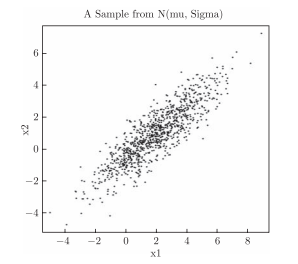
As an example, consider a bivariate normal random vector $\mathrm{x}=\left(x_{1}, x_{2}\right)^{\mathrm{T}}$ with the mean vector and covariance matrix given by
$$
\boldsymbol{\mu}=\left(\begin{array}{l}
2 \
1
\end{array}\right), \quad \Sigma=\left(\begin{array}{ll}
4 & 3 \
3 & 3
\end{array}\right)
$$
Then, we have $x_{1} \sim N(2,4), x_{2} \sim N(1,3)$, and the correlation between $x_{1}$ and $x_{2}$ is
$$
r=\frac{\operatorname{Cov}\left(x_{1}, x_{2}\right)}{\sqrt{\operatorname{Var}\left(x_{1}\right) \operatorname{Var}\left(x_{2}\right)}}=\frac{3}{\sqrt{4 \times 3}}=0.866 .
$$
统计代写|多元统计分析代写Multivariate Statistical Analysis代考|Properties of multivariate normal distributions
Since the multivariate normal distribution is the most important distribution for multivariate continuous data, we list some of its important properties, which are useful in multivariate analysis. Note that properties (i) and (ii) below do not require that the distribution is normal.
Let $\mathbf{x}$ and $\mathbf{y}$ be two random vectors, and let $B$ and $\mathbf{b}$ be a constant matrix and a constant vector respectively, Let $\mathbf{y}=\boldsymbol{B x}+\mathbf{b}$ be a linear transformation. Then, we have the following properties:
(i) $E(\mathbf{y})=\boldsymbol{B E}(\mathbf{x})+\mathbf{b}$;
(ii) $\operatorname{Cov}(\mathbf{y})=\boldsymbol{B C o v}(\mathbf{x}) \boldsymbol{B}^{\mathrm{T}}$;
(iii) If $\mathbf{x} \sim N_{p}(\boldsymbol{\mu}, \Sigma)$, then
$$
\mathbf{y}=\boldsymbol{B x}+\mathbf{b} \sim N\left(\boldsymbol{B} \boldsymbol{\mu}+\mathbf{b}, \boldsymbol{B} \Sigma \boldsymbol{B}^{\mathrm{T}}\right)
$$
i.e., a linear transformation of a normal random vector is still normally distributed;
(iv) If $\mathrm{x} \sim N_{p}(\boldsymbol{\mu}, \Sigma)$ and
$$
\mathbf{x}=\left(\begin{array}{l}
\mathbf{x}{1} \ \mathbf{x}{2}
\end{array}\right), \quad \mu=\left(\begin{array}{l}
\mu_{1} \
\mu_{2}
\end{array}\right), \quad \Sigma=\left(\begin{array}{ll}
\Sigma_{11} & \Sigma_{12} \
\Sigma_{21} & \Sigma_{22}
\end{array}\right)
$$
then
$$
\mathbf{x}{1} \sim N\left(\mu{1}, \Sigma_{11}\right), \quad \mathbf{x}{2} \sim N\left(\mu{2}, \Sigma_{22}\right),
$$
and the conditional distribution of $\mathbf{x}{1}$ given $\mathbf{x}{2}$ is still normally distributed and is given by
$$
\mathbf{x}{1} \mid \mathbf{x}{2} \sim N\left(\mu_{1}+\Sigma_{12} \Sigma_{22}^{-1}\left(\mathbf{x}{2}-\mu{2}\right), \Sigma_{11.2}\right),
$$ where $\Sigma_{11,2}=\Sigma_{11}-\Sigma_{12} \Sigma_{22}^{-1} \Sigma_{21}$. In other words, for a multivariate normal distribution, its components’ distributions and conditional distributions are still normal.
多元统计分析代考
统计代写|多元统计分析代写Multivariate Statistical Analysis代考|Covariance matrix and correlation matrix
由于多变量分析的主要焦点是合并变量之间的相关性,因此协方差矩阵或相关矩阵在连续数据或变量的多变量分析中起着重要作用。假设X和是是两个连续的随机变量,假设\left{x_{1}, x_{2}, \cdots, x_{n}\right}\left{x_{1}, x_{2}, \cdots, x_{n}\right}和\left{y_{1}, y_{2}, \cdots, y_{n}\right}\left{y_{1}, y_{2}, \cdots, y_{n}\right}收集的数据是X和是分别。之间的相关性X和是可以通过协方差来衡量这(X,是)或相关系数r :
这(X,是)=和[(X−和(X))(是−和(是))], r=这(X,是)σXσ是
在哪里σX=曾是(X)和σ是=曾是(是)是标准差X和是分别。相关系数r是一个介于−1和 1 ,它衡量两个变量之间的线性相关性。如果r>0,X和是是正相关的。如果r<0,X和是是负相关的。值越大|r|,相关性越强。什么时候r=0,X和是不是线性相关的。
注意相关系数r只测量线性关系,而不是其他关系,即观察值X和是大致落在一条直线上。例如,当r=0,X和是可能仍然存在非线性关系。
更一般地,让X=(X1,X2,⋯,Xp)吨是一个随机向量p连续随机变量。的平均向量X是
和(X)=μ=(μ1,μ2,⋯,μp)吨
的协方差矩阵X由
$$
\Sigma=\operatorname{Cov}(\mathbf{X})=\left(\sigma_{ij}\right) {p \times p}, \quad \text { where } \quad \sigma 给出{ij}=E\left(X_{i}-E\left(X_{i}\right)\right)\left(X_{j}-E\left(X_{j}\right)\right)
$ $
以及之间的相关性X一世和Xj是
r一世j=σ一世jσ一世一世σjj,一世,j=1,2,⋯,p.
统计代写|多元统计分析代写Multivariate Statistical Analysis代考|Multivariate Normal Distribution
在前面的部分中,我们不假设随机变量或数据的任何参数分布。然而,当我们执行假设检验等统计推断时,我们需要假设多元数据遵循一些参数分布。连续多元数据最常见的分布是多元正态分布。有几个原因。首先,根据中心极限定理,即使原始数据不服从正态分布,许多统计量(例如样本均值)也会渐近服从正态分布。换句话说,当样本量很大时,正态性假设对于这些统计数据可能是合理的。其次,正态分布具有许多吸引人的特性。例如,一个正态分布完全由它的均值和方差(协方差)决定,这是数据最重要的两个特征。第三,许多连续数据,即使它们可能不是正态分布的,也可以转换为大致正态分布的数据。例如,我们可以考虑对正数(例如年龄)或偏斜数据(例如生存时间)进行对数转换。最后,对于多元连续数据,没有多少合理的多元分布可供选择。因此,对于多元连续数据,如果统计推断需要一个分布假设,我们经常假设数据服从多元正态分布。但是请注意,这只是一个假设,因此需要根据数据检查其有效性。可以转化为大致正态分布的数据。例如,我们可以考虑对正数(例如年龄)或偏斜数据(例如生存时间)进行对数转换。最后,对于多元连续数据,没有多少合理的多元分布可供选择。因此,对于多元连续数据,如果统计推断需要一个分布假设,我们经常假设数据服从多元正态分布。但是请注意,这只是一个假设,因此需要根据数据检查其有效性。可以转化为大致正态分布的数据。例如,我们可以考虑对正数(例如年龄)或偏斜数据(例如生存时间)进行对数转换。最后,对于多元连续数据,没有多少合理的多元分布可供选择。因此,对于多元连续数据,如果统计推断需要一个分布假设,我们经常假设数据服从多元正态分布。但是请注意,这只是一个假设,因此需要根据数据检查其有效性。没有多少合理的多元分布可供选择。因此,对于多元连续数据,如果统计推断需要一个分布假设,我们经常假设数据服从多元正态分布。但是请注意,这只是一个假设,因此需要根据数据检查其有效性。没有多少合理的多元分布可供选择。因此,对于多元连续数据,如果统计推断需要一个分布假设,我们经常假设数据服从多元正态分布。但是请注意,这只是一个假设,因此需要根据数据检查其有效性。
随机向量X=(X1,⋯,Xp)吨遵循一个p维多元正态分布,表示为ñp(μ,Σ),如果随机向量的分量的任何线性组合X服从单变量正态分布。也就是说,对于任何常数
向量一个=(一个1,一个2,⋯,一个p)吨, 单变量随机变量是=一个吨X=∑一世=1p一个一世X一世服从单变量正态分布
一个吨X∼ñ(∑一世=1p一个一世和(X一世),曾是(∑一世=1p一个一世X一世))
因此,如果X跟随ñp(μ,Σ), 每个分量Xķ跟随ñ(μķ,σķķ),ķ=1,⋯,p. 请注意,反过来可能不正确:如果每个Xķ跟随ñ(μķ,σķķ), x 可能服从也可能不服从正态分布。的概率密度函数X∼ñp(μ,Σ)可以写成
F(X)=1(2圆周率)p/2|Σ|1/2经验[−12(X−μ)吨Σ−1(X−μ)] −∞<Xj<∞,j=1,2,⋯,p
当p=1.
例如,考虑一个二元正态随机向量X=(X1,X2)吨平均向量和协方差矩阵由下式给出
μ=(2 1),Σ=(43 33)
那么,我们有X1∼ñ(2,4),X2∼ñ(1,3),以及之间的相关性X1和X2是
r=这(X1,X2)曾是(X1)曾是(X2)=34×3=0.866.
统计代写|多元统计分析代写Multivariate Statistical Analysis代考|Properties of multivariate normal distributions
由于多元正态分布是多元连续数据最重要的分布,我们列出了它的一些重要性质,这些性质在多元分析中很有用。请注意,下面的属性 (i) 和 (ii) 并不要求分布是正态的。
让X和是是两个随机向量,让乙和b分别是一个常数矩阵和一个常数向量,令是=乙X+b是一个线性变换。然后,我们有以下性质:
(i)和(是)=乙和(X)+b;
(二)这(是)=乙C○在(X)乙吨;
(iii) 如果X∼ñp(μ,Σ), 然后
是=乙X+b∼ñ(乙μ+b,乙Σ乙吨)
即一个正态随机向量的线性变换仍然是正态分布的;
(iv) 如果X∼ñp(μ,Σ)和
X=(X1 X2),μ=(μ1 μ2),Σ=(Σ11Σ12 Σ21Σ22)
然后
X1∼ñ(μ1,Σ11),X2∼ñ(μ2,Σ22),
和条件分布X1给定X2仍然是正态分布的并且由下式给出
X1∣X2∼ñ(μ1+Σ12Σ22−1(X2−μ2),Σ11.2),在哪里Σ11,2=Σ11−Σ12Σ22−1Σ21. 换句话说,对于一个多元正态分布,它的分量分布和条件分布仍然是正态的。

统计代写请认准statistics-lab™. statistics-lab™为您的留学生涯保驾护航。
金融工程代写
金融工程是使用数学技术来解决金融问题。金融工程使用计算机科学、统计学、经济学和应用数学领域的工具和知识来解决当前的金融问题,以及设计新的和创新的金融产品。
非参数统计代写
非参数统计指的是一种统计方法,其中不假设数据来自于由少数参数决定的规定模型;这种模型的例子包括正态分布模型和线性回归模型。
广义线性模型代考
广义线性模型(GLM)归属统计学领域,是一种应用灵活的线性回归模型。该模型允许因变量的偏差分布有除了正态分布之外的其它分布。
术语 广义线性模型(GLM)通常是指给定连续和/或分类预测因素的连续响应变量的常规线性回归模型。它包括多元线性回归,以及方差分析和方差分析(仅含固定效应)。
有限元方法代写
有限元方法(FEM)是一种流行的方法,用于数值解决工程和数学建模中出现的微分方程。典型的问题领域包括结构分析、传热、流体流动、质量运输和电磁势等传统领域。
有限元是一种通用的数值方法,用于解决两个或三个空间变量的偏微分方程(即一些边界值问题)。为了解决一个问题,有限元将一个大系统细分为更小、更简单的部分,称为有限元。这是通过在空间维度上的特定空间离散化来实现的,它是通过构建对象的网格来实现的:用于求解的数值域,它有有限数量的点。边界值问题的有限元方法表述最终导致一个代数方程组。该方法在域上对未知函数进行逼近。[1] 然后将模拟这些有限元的简单方程组合成一个更大的方程系统,以模拟整个问题。然后,有限元通过变化微积分使相关的误差函数最小化来逼近一个解决方案。
tatistics-lab作为专业的留学生服务机构,多年来已为美国、英国、加拿大、澳洲等留学热门地的学生提供专业的学术服务,包括但不限于Essay代写,Assignment代写,Dissertation代写,Report代写,小组作业代写,Proposal代写,Paper代写,Presentation代写,计算机作业代写,论文修改和润色,网课代做,exam代考等等。写作范围涵盖高中,本科,研究生等海外留学全阶段,辐射金融,经济学,会计学,审计学,管理学等全球99%专业科目。写作团队既有专业英语母语作者,也有海外名校硕博留学生,每位写作老师都拥有过硬的语言能力,专业的学科背景和学术写作经验。我们承诺100%原创,100%专业,100%准时,100%满意。
随机分析代写
随机微积分是数学的一个分支,对随机过程进行操作。它允许为随机过程的积分定义一个关于随机过程的一致的积分理论。这个领域是由日本数学家伊藤清在第二次世界大战期间创建并开始的。
时间序列分析代写
随机过程,是依赖于参数的一组随机变量的全体,参数通常是时间。 随机变量是随机现象的数量表现,其时间序列是一组按照时间发生先后顺序进行排列的数据点序列。通常一组时间序列的时间间隔为一恒定值(如1秒,5分钟,12小时,7天,1年),因此时间序列可以作为离散时间数据进行分析处理。研究时间序列数据的意义在于现实中,往往需要研究某个事物其随时间发展变化的规律。这就需要通过研究该事物过去发展的历史记录,以得到其自身发展的规律。
回归分析代写
多元回归分析渐进(Multiple Regression Analysis Asymptotics)属于计量经济学领域,主要是一种数学上的统计分析方法,可以分析复杂情况下各影响因素的数学关系,在自然科学、社会和经济学等多个领域内应用广泛。
MATLAB代写
MATLAB 是一种用于技术计算的高性能语言。它将计算、可视化和编程集成在一个易于使用的环境中,其中问题和解决方案以熟悉的数学符号表示。典型用途包括:数学和计算算法开发建模、仿真和原型制作数据分析、探索和可视化科学和工程图形应用程序开发,包括图形用户界面构建MATLAB 是一个交互式系统,其基本数据元素是一个不需要维度的数组。这使您可以解决许多技术计算问题,尤其是那些具有矩阵和向量公式的问题,而只需用 C 或 Fortran 等标量非交互式语言编写程序所需的时间的一小部分。MATLAB 名称代表矩阵实验室。MATLAB 最初的编写目的是提供对由 LINPACK 和 EISPACK 项目开发的矩阵软件的轻松访问,这两个项目共同代表了矩阵计算软件的最新技术。MATLAB 经过多年的发展,得到了许多用户的投入。在大学环境中,它是数学、工程和科学入门和高级课程的标准教学工具。在工业领域,MATLAB 是高效研究、开发和分析的首选工具。MATLAB 具有一系列称为工具箱的特定于应用程序的解决方案。对于大多数 MATLAB 用户来说非常重要,工具箱允许您学习和应用专业技术。工具箱是 MATLAB 函数(M 文件)的综合集合,可扩展 MATLAB 环境以解决特定类别的问题。可用工具箱的领域包括信号处理、控制系统、神经网络、模糊逻辑、小波、仿真等。