如果你也在 怎样代写多元统计分析Multivariate Statistical Analysis这个学科遇到相关的难题,请随时右上角联系我们的24/7代写客服。
多变量统计分析被认为是评估地球化学异常与任何单独变量和变量之间相互影响的意义的有用工具。
statistics-lab™ 为您的留学生涯保驾护航 在代写多元统计分析Multivariate Statistical Analysis方面已经树立了自己的口碑, 保证靠谱, 高质且原创的统计Statistics代写服务。我们的专家在代写多元统计分析Multivariate Statistical Analysis代写方面经验极为丰富,各种代写多元统计分析Multivariate Statistical Analysis相关的作业也就用不着说。
我们提供的多元统计分析Multivariate Statistical Analysis及其相关学科的代写,服务范围广, 其中包括但不限于:
- Statistical Inference 统计推断
- Statistical Computing 统计计算
- Advanced Probability Theory 高等概率论
- Advanced Mathematical Statistics 高等数理统计学
- (Generalized) Linear Models 广义线性模型
- Statistical Machine Learning 统计机器学习
- Longitudinal Data Analysis 纵向数据分析
- Foundations of Data Science 数据科学基础
统计代写|多元统计分析代写Multivariate Statistical Analysis代考|Check for Multivariate Normality
When we assume a multivariate normal distribution for data analysis, we should check to see if this assumption is supported by the data. Unlike univariate normal distribution, it is not straightforward to check multivariate normal distributional assumption. In the following, we discuss methods that may be used to check multivariate normality.
First, as a simple and naive approach, we may consider methods for checking univariate normality, which may also be useful for checking multivariate normality, Note that, if observations were generated from a multivariate normal distribution, then each univariate distribution will also be normal. In other words, if the univariate data are not normally distributed, then the multivariate data will not be normally distributed either. Boxplots and histograms can be used to check if the univariate data are symmetric or not (note that all normal data are symmetric), but symmetric data are not necessarily normal. If the univariate data are not symmetric, then the normality cannot hold. A more formal method to check univariate normality is normal quantile-quantile (Q-Q) plot. A normal $Q$ – $Q$ plots shows the theoretical quantiles from a normal distribution and the quantiles computed from the data. If a Q-Q plot shows a straight line $(y=x)$, then the univariate data may be considered as normally distributed. A more formal method, called the Shapiro-Wilk test, may also be used to check normality.
A formal method for checking multivariate normality is the Chi-Squared plot. It is a generalization of a Q-Q plot based on the squared Mahalanobis distance
$$
d_{j}^{2}=\left(\mathbf{x}{j}-\overline{\mathbf{x}}\right)^{\mathrm{T}} \boldsymbol{S}^{-1}\left(\mathbf{x}{j}-\overline{\mathbf{x}}\right), \quad j=1,2, \cdots, n
$$
where $\mathbf{x}{1}, \mathbf{x}{2}, \cdots, \mathbf{x}{n}$ are the sample observations, $\overline{\mathbf{x}}$ is the sample mean vector, and $S$ is the sample covariance matrix. If the population is multivariate normal and $n-p$ is large, each of the squared distances $d{1}^{2}, d_{2}^{2}, \cdots, d_{n}^{2}$ should behave as a chi-square random variable. We can order the squared distances as $d_{(1)}^{2} \leqslant d_{(2)}^{2} \leqslant \cdots \leqslant d_{(n)}^{2}$, and then graph the pairs $\left(q((j-1 / 2) / n), d_{(j)}^{2}\right)$, where $q((j-1 / 2) / n)$ is the $(j-1 / 2) / n$ quantile of the chi-square distribution with $p$ degrees of freedom. Under multivariate normality, the plot should resemble a straight line through the origin with slope 1 . A systematic curved pattern indicates that normality may not hold. A few points far above the line suggests outliers. We give an example below.
To illustrate the idea of the Chi-Squared plot, we simulate a sample of size 100 from the bivariate normal distribution $\left(x_{1}, x_{2}\right) \sim N_{2}(\boldsymbol{\mu}, \Sigma)$, with the mean vector and the covariance matrix given by
$$
\mu=\left(\begin{array}{c}
-1 \
1
\end{array}\right), \quad \Sigma=\left(\begin{array}{cc}
10 & -3 \
-3 & 2
\end{array}\right)
$$
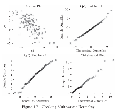
Then we draw Q-Q plots to verify univariate normalities of the component random variables $x_{1}$ and $x_{2}$ respectively, and draw a Chi-Squared plot to verify the bivariate normality of the random vector $\left(x_{1}, x_{2}\right)$. See Figure $1.7$. The $\mathrm{R}$ code is given below.
统计代写|多元统计分析代写Multivariate Statistical Analysis代考|Unsupervised Learning and Supervised Learning
Statistics is about learning from data. In practice, data are often collected on more than one variables, so many statistical methods may be viewed as multivariate analysis in a broad sense. In general, we may classify these methods into two general approaches:
- Unsupervised learning: we treat all variables symmetrically or equally, with the goal of understanding the underlying association structures between these variables. Examples of unsupervised learning include principal components analysis, factor analysis, and cluster analysis.
- Supervised learning: we treat one or more variables as responses and other variables as predictors which are used to partially explain the variations in the responses. Regression models are examples of supervised learning.
These two approaches are used to answer different questions, so the choice of methods depends on the study objectives. There is a wide variety of statistical methods available for each approach. If our goal is to understand the relationship among all the variables or if we want to reduce the number of variables, we should consider unsupervised learning methods. If our objective is to predict one or more variables using the other variables or to explain the variations in one or more variables using other variables, we should use regression models.
In unsupervised learning, all variables are treated equally and the goal is to understand the covariance structures in these variables or to reduce the dimension of the data space. Commonly used unsupervised learning methods for multivariate continuous data include principal components analysis (PCA), factor analysis, discriminant analysis, and cluster analysis, For example, in PCA and factor analysis, the original set of variables can be replaced by a smaller set of new variables which may explain most of the variation in the original data. These new variables are usually special linear combinations of the original variables, and they allow us to use graphical tools to display the data and to interpret the data more easily than the original sets of variables. In discriminant analysis and cluster analysis, we classify multivariate data into different clusters based on the “distances” between the observations. In these proce-
dures, distributional assumptions for the data may not be needed. The covariance matrices or correlation matrices play the key role.
Regression models are among the most useful statistical methods. There are many types of regression models. The types of regression models are determined based on the types of the response variables, not the types of predictors. For example, if the response is a continuous variable, we may consider a linear regression model, but if the response is a binary (discrete) variable, we may consider a logistic regression model. The following regression models are commonly used in practice; linear models, nonlinear models, generalized linear models, survival models, and models for longitudinal data or clustered data. Linear regression models are often considered when the response variables are continuous and roughly normally distributed. Analysis of variance (ANOVA) models are special linear models in which all predictors are categorical or discrete. Nonlinear regression models may be used when the response variables are continuous and roughly normally distributed, and there is a good understanding of the mechanisms that generate the data. Generalized linear models (GLMs) are often used when the response variables are binary or count or follow distributions in the exponential family. Survival models are used when the response variables are the times to some events of interest, such as times to death or times to accidents. The foregoing regression models are used for independent data. When the data are correlated or clustered, we should use models for clustered data.
In a regression model, if there are more than one response variables, the model is called a multivariate regression model. For example, if there are two or more responses in an ANOVA model, the model is called a multivariate $A N O V A$ (MANOVA) model.
统计代写|多元统计分析代写Multivariate Statistical Analysis代考|Statistical Inference
A main goal of statistical inference is to generalize the results obtained from a sample to the general population. To achieve this, the sample has to be representative of the population, and the data are assumed to follow some parametric distributions such as normal distributions. Such an assumption allows us to do probability calculation required in inference (e.g., p-values in hypothesis testing).
Multivariate continuous data are often assumed to follow multivariate normal distributions. Under this distributional assumption, we can perform usual statistical inference, such as confidence regions and hypothesis testing for the unknown population mean vectors or the covariance matrices. For example, for univariate continuous data, the most well-known test is perhaps the $t$-test for the population mean, while for multivariate continuous data, the most well-known test is perhaps the Hotelling’s $T^{2}$-test for the mean vector. A major consideration in multivariate analysis is to incorporate the correlation between the variables. This allows for more efficient inference
than univariate analysis, which ignores the correlation between variables,
Multivariate discrete data are often assumed to follow multinomial distributions. Under this distributional assumption, statistical inference for the unknown parameters can be done using standard methods such as the maximum likelihood method. The simplest and also the most common multivariate discrete data are often summarized by $2 \times 2$ tables. For example, we may want to compare two methods, with the response being either positive or negative. The results can then be summarized by a $2 \times 2$ table. Many statistical methods are available to analyze such $2 \times 2$ tables. More general multivariate discrete data may be summarized by $k \times m$ contingency tables.
多元统计分析代考
统计代写|多元统计分析代写Multivariate Statistical Analysis代考|Check for Multivariate Normality
当我们假设数据分析的多元正态分布时,我们应该检查数据是否支持这个假设。与单变量正态分布不同,检查多元正态分布假设并不简单。在下文中,我们将讨论可用于检查多元正态性的方法。
首先,作为一种简单而朴素的方法,我们可以考虑检查单变量正态性的方法,这也可能对检查多变量正态性有用。请注意,如果观测值是从多元正态分布生成的,那么每个单变量分布也将是正态的。换句话说,如果单变量数据不是正态分布的,那么多元数据也不会是正态分布的。箱线图和直方图可用于检查单变量数据是否对称(注意所有正态数据都是对称的),但对称数据不一定是正态的。如果单变量数据不对称,则正态性不能成立。检查单变量正态性的更正式的方法是正态分位数 – 分位数 (QQ) 图。一个正常的问 – 问绘图显示来自正态分布的理论分位数和根据数据计算的分位数。如果 QQ 图显示一条直线(是=X),那么单变量数据可以被认为是正态分布的。一种更正式的方法,称为 Shapiro-Wilk 检验,也可用于检查正态性。
检查多元正态性的正式方法是卡方图。它是基于平方马氏距离的 QQ 图的推广
dj2=(Xj−X¯)吨小号−1(Xj−X¯),j=1,2,⋯,n
在哪里X1,X2,⋯,Xn是样本观测值,X¯是样本均值向量,并且小号是样本协方差矩阵。如果总体是多元正态且n−p很大,每个平方距离d12,d22,⋯,dn2应该表现为卡方随机变量。我们可以将平方距离排序为d(1)2⩽d(2)2⩽⋯⩽d(n)2,然后绘制成对(q((j−1/2)/n),d(j)2), 在哪里q((j−1/2)/n)是个(j−1/2)/n卡方分布的分位数p自由程度。在多元正态性下,该图应类似于通过原点的直线,斜率为 1 。系统的弯曲模式表明常态可能不成立。远高于该线的几个点表明异常值。我们在下面举一个例子。
为了说明卡方图的概念,我们从二元正态分布中模拟大小为 100 的样本(X1,X2)∼ñ2(μ,Σ), 均值向量和协方差矩阵由下式给出
μ=(−1 1),Σ=(10−3 −32)
然后我们绘制QQ图来验证分量随机变量的单变量正态性X1和X2分别绘制卡方图来验证随机向量的二元正态性(X1,X2). 见图1.7. 这R代码如下。
统计代写|多元统计分析代写Multivariate Statistical Analysis代考|Unsupervised Learning and Supervised Learning
统计学是关于从数据中学习的。在实践中,数据往往是针对多个变量收集的,因此许多统计方法可以被视为广义上的多变量分析。一般来说,我们可以将这些方法分为两种一般方法:
- 无监督学习:我们对称或平等地对待所有变量,目的是了解这些变量之间的潜在关联结构。无监督学习的例子包括主成分分析、因子分析和聚类分析。
- 监督学习:我们将一个或多个变量视为响应,将其他变量视为预测变量,用于部分解释响应的变化。回归模型是监督学习的例子。
这两种方法用于回答不同的问题,因此方法的选择取决于研究目标。每种方法都有多种统计方法可用。如果我们的目标是了解所有变量之间的关系,或者如果我们想减少变量的数量,我们应该考虑无监督学习方法。如果我们的目标是使用其他变量来预测一个或多个变量,或者使用其他变量来解释一个或多个变量的变化,我们应该使用回归模型。
在无监督学习中,所有变量都被平等对待,目标是理解这些变量中的协方差结构或减少数据空间的维度。多变量连续数据常用的无监督学习方法包括主成分分析(PCA)、因子分析、判别分析和聚类分析,例如,在主成分分析和因子分析中,可以用较小的一组新变量代替原来的一组变量。可以解释原始数据中大部分变化的变量。这些新变量通常是原始变量的特殊线性组合,它们允许我们使用图形工具来显示数据并比原始变量集更容易地解释数据。在判别分析和聚类分析中,我们根据观测值之间的“距离”将多元数据分类到不同的集群中。在这些过程中
时,可能不需要数据的分布假设。协方差矩阵或相关矩阵起关键作用。
回归模型是最有用的统计方法之一。有许多类型的回归模型。回归模型的类型取决于响应变量的类型,而不是预测变量的类型。例如,如果响应是连续变量,我们可以考虑线性回归模型,但如果响应是二元(离散)变量,我们可以考虑逻辑回归模型。以下回归模型在实践中常用;线性模型、非线性模型、广义线性模型、生存模型和纵向数据或聚类数据模型。当响应变量是连续的且大致呈正态分布时,通常会考虑线性回归模型。方差分析 (ANOVA) 模型是特殊的线性模型,其中所有预测变量都是分类的或离散的。当响应变量是连续的且大致呈正态分布时,可以使用非线性回归模型,并且对生成数据的机制有很好的理解。当响应变量是二进制或计数或遵循指数族的分布时,通常使用广义线性模型 (GLM)。当响应变量是某些感兴趣事件的时间(例如死亡时间或事故时间)时,使用生存模型。上述回归模型用于独立数据。当数据相关或聚类时,我们应该对聚类数据使用模型。当响应变量是二进制或计数或遵循指数族的分布时,通常使用广义线性模型 (GLM)。当响应变量是某些感兴趣事件的时间(例如死亡时间或事故时间)时,使用生存模型。上述回归模型用于独立数据。当数据相关或聚类时,我们应该对聚类数据使用模型。当响应变量是二进制或计数或遵循指数族的分布时,通常使用广义线性模型 (GLM)。当响应变量是某些感兴趣事件的时间(例如死亡时间或事故时间)时,使用生存模型。上述回归模型用于独立数据。当数据相关或聚类时,我们应该对聚类数据使用模型。
在回归模型中,如果存在多个响应变量,则该模型称为多元回归模型。例如,如果 ANOVA 模型中有两个或多个响应,则该模型称为多变量一个ñ○在一个(MANOVA) 模型。
统计代写|多元统计分析代写Multivariate Statistical Analysis代考|Statistical Inference
统计推断的主要目标是将从样本中获得的结果推广到一般人群。为了实现这一点,样本必须代表总体,并且假设数据遵循一些参数分布,例如正态分布。这样的假设允许我们进行推理所需的概率计算(例如,假设检验中的 p 值)。
通常假设多元连续数据遵循多元正态分布。在这种分布假设下,我们可以执行通常的统计推断,例如对未知总体均值向量或协方差矩阵的置信区域和假设检验。例如,对于单变量连续数据,最著名的检验可能是吨- 检验总体均值,而对于多变量连续数据,最著名的检验可能是 Hotelling 检验吨2- 测试平均向量。多变量分析的一个主要考虑因素是纳入变量之间的相关性。这允许更有效的推理
与忽略变量之间相关性的单变量分析相比,
通常假设多变量离散数据遵循多项分布。在这种分布假设下,可以使用最大似然法等标准方法对未知参数进行统计推断。最简单也是最常见的多元离散数据通常总结为2×2表。例如,我们可能想要比较两种方法,响应是肯定的或否定的。然后可以将结果总结为2×2桌子。有许多统计方法可用于分析此类2×2表。更一般的多元离散数据可以总结为ķ×米列联表。

统计代写请认准statistics-lab™. statistics-lab™为您的留学生涯保驾护航。
金融工程代写
金融工程是使用数学技术来解决金融问题。金融工程使用计算机科学、统计学、经济学和应用数学领域的工具和知识来解决当前的金融问题,以及设计新的和创新的金融产品。
非参数统计代写
非参数统计指的是一种统计方法,其中不假设数据来自于由少数参数决定的规定模型;这种模型的例子包括正态分布模型和线性回归模型。
广义线性模型代考
广义线性模型(GLM)归属统计学领域,是一种应用灵活的线性回归模型。该模型允许因变量的偏差分布有除了正态分布之外的其它分布。
术语 广义线性模型(GLM)通常是指给定连续和/或分类预测因素的连续响应变量的常规线性回归模型。它包括多元线性回归,以及方差分析和方差分析(仅含固定效应)。
有限元方法代写
有限元方法(FEM)是一种流行的方法,用于数值解决工程和数学建模中出现的微分方程。典型的问题领域包括结构分析、传热、流体流动、质量运输和电磁势等传统领域。
有限元是一种通用的数值方法,用于解决两个或三个空间变量的偏微分方程(即一些边界值问题)。为了解决一个问题,有限元将一个大系统细分为更小、更简单的部分,称为有限元。这是通过在空间维度上的特定空间离散化来实现的,它是通过构建对象的网格来实现的:用于求解的数值域,它有有限数量的点。边界值问题的有限元方法表述最终导致一个代数方程组。该方法在域上对未知函数进行逼近。[1] 然后将模拟这些有限元的简单方程组合成一个更大的方程系统,以模拟整个问题。然后,有限元通过变化微积分使相关的误差函数最小化来逼近一个解决方案。
tatistics-lab作为专业的留学生服务机构,多年来已为美国、英国、加拿大、澳洲等留学热门地的学生提供专业的学术服务,包括但不限于Essay代写,Assignment代写,Dissertation代写,Report代写,小组作业代写,Proposal代写,Paper代写,Presentation代写,计算机作业代写,论文修改和润色,网课代做,exam代考等等。写作范围涵盖高中,本科,研究生等海外留学全阶段,辐射金融,经济学,会计学,审计学,管理学等全球99%专业科目。写作团队既有专业英语母语作者,也有海外名校硕博留学生,每位写作老师都拥有过硬的语言能力,专业的学科背景和学术写作经验。我们承诺100%原创,100%专业,100%准时,100%满意。
随机分析代写
随机微积分是数学的一个分支,对随机过程进行操作。它允许为随机过程的积分定义一个关于随机过程的一致的积分理论。这个领域是由日本数学家伊藤清在第二次世界大战期间创建并开始的。
时间序列分析代写
随机过程,是依赖于参数的一组随机变量的全体,参数通常是时间。 随机变量是随机现象的数量表现,其时间序列是一组按照时间发生先后顺序进行排列的数据点序列。通常一组时间序列的时间间隔为一恒定值(如1秒,5分钟,12小时,7天,1年),因此时间序列可以作为离散时间数据进行分析处理。研究时间序列数据的意义在于现实中,往往需要研究某个事物其随时间发展变化的规律。这就需要通过研究该事物过去发展的历史记录,以得到其自身发展的规律。
回归分析代写
多元回归分析渐进(Multiple Regression Analysis Asymptotics)属于计量经济学领域,主要是一种数学上的统计分析方法,可以分析复杂情况下各影响因素的数学关系,在自然科学、社会和经济学等多个领域内应用广泛。
MATLAB代写
MATLAB 是一种用于技术计算的高性能语言。它将计算、可视化和编程集成在一个易于使用的环境中,其中问题和解决方案以熟悉的数学符号表示。典型用途包括:数学和计算算法开发建模、仿真和原型制作数据分析、探索和可视化科学和工程图形应用程序开发,包括图形用户界面构建MATLAB 是一个交互式系统,其基本数据元素是一个不需要维度的数组。这使您可以解决许多技术计算问题,尤其是那些具有矩阵和向量公式的问题,而只需用 C 或 Fortran 等标量非交互式语言编写程序所需的时间的一小部分。MATLAB 名称代表矩阵实验室。MATLAB 最初的编写目的是提供对由 LINPACK 和 EISPACK 项目开发的矩阵软件的轻松访问,这两个项目共同代表了矩阵计算软件的最新技术。MATLAB 经过多年的发展,得到了许多用户的投入。在大学环境中,它是数学、工程和科学入门和高级课程的标准教学工具。在工业领域,MATLAB 是高效研究、开发和分析的首选工具。MATLAB 具有一系列称为工具箱的特定于应用程序的解决方案。对于大多数 MATLAB 用户来说非常重要,工具箱允许您学习和应用专业技术。工具箱是 MATLAB 函数(M 文件)的综合集合,可扩展 MATLAB 环境以解决特定类别的问题。可用工具箱的领域包括信号处理、控制系统、神经网络、模糊逻辑、小波、仿真等。