如果你也在 怎样代写实验设计与分析Design and Analysis of Experiments这个学科遇到相关的难题,请随时右上角联系我们的24/7代写客服。
实验设计与分析提供了一个严格的介绍,通过质量和性能优化来改进产品和工艺设计。
statistics-lab™ 为您的留学生涯保驾护航 在代写实验设计与分析Design and Analysis of Experiments方面已经树立了自己的口碑, 保证靠谱, 高质且原创的统计Statistics代写服务。我们的专家在代写实验设计与分析Design and Analysis of Experiments方面经验极为丰富,各种代写实验设计与分析Design and Analysis of Experiments相关的作业也就用不着说。
我们提供的实验设计与分析Design and Analysis of Experiments及其相关学科的代写,服务范围广, 其中包括但不限于:
- Statistical Inference 统计推断
- Statistical Computing 统计计算
- Advanced Probability Theory 高等楖率论
- Advanced Mathematical Statistics 高等数理统计学
- (Generalized) Linear Models 广义线性模型
- Statistical Machine Learning 统计机器学习
- Longitudinal Data Analysis 纵向数据分析
- Foundations of Data Science 数据科学基础
统计代写|实验设计与分析作业代写Design and Analysis of Experiments代考|All Crops in a Mixture
The simplest form of intercropping with three or more crops in the mixture and with one major crop and two or more minor crops was considered in Chapter 12. The complexity of the statistical analyses over that in Chapter 2 (two crops) of Volume I is increased. The methods of Chapters 3 and 4 of Volume I were extended to mixtures of three or more crops in Chapter 13. Analyses for individual crop responses for each crop as well as analyses for combined responses for all crops in the mixture are presented. The density for a given crop in the mixture was held constant from mixture to mixture. In the present chapter, cropping systems which allow varying densities for some or all crops are considered. The methods presented herein are a generalization of those presented in Chapter 5 of Volume I.
Many patterns for varying and/or constant densities in a mixture are possible. The particular densities selected for study will depend on the makeup of the crop mixture as well as the goals of the experiment. With one major crop and two or more minor crops:
(i) The density of the major crop could be varied and the densities of the minor crops kept constant.
(ii) The density of the major crop could be held constant and some or all of the densities of the minor crops varied.
(iii) The densities of all crops in the mixture could be varied.
With three or more major crops and with some or no minor crops in a mixture, the following situations are possible:
78
- Varying Densities for Some or All Crops in a Mixture
(i) The densities of all major crops in the mixture could be varied.
(ii) The densities of two or more major crops could be constant and the densities of the remaining crops could be varied.
(iii) The densities of any minor crops included in (i) or (ii) could be varied or held constant. - As discussed in Chapter 5 of Volume I, serious attention needs to be given to selecting the various density levels for each crop. The experimenter needs to decide whether to make the levels selected for one crop dependent or independent of the levels selected for the remaining crops in a mixture. It may make sense to approach a maximum density for all crops in the mixture as the total number of plants, regardless of crop, is the total population level beyond which there will be no increased yields. The amount of moisture, plant nutrients, sunlight, etc. may dictate the maximum population level that can be supported on a plot of ground. It is well known that overpopulation can result in reduced or even zero yields. In order to pinpoint density levels producing maximum or nearmaximum responses, it is advisable to select levels somewhat beyond the level giving maximum response. For example, the maximum yield of maize may be attained with 60,000 plants per hectare. A level of 70,000 , or even 80,000 , plants per hectare should result in decreased yields and should be included for study in an experiment. In determining response curves, experimenters often make the mistake of including only levels which “would be used in practice.” The inclusion of levels beyond those normally used in practice results in a more accurate response curve showing the relationship between response and density level. If a response curve does not show a decrease at the highest density, it is not clear that the maximum has been attained and that higher density levels should have been included.
统计代写|实验设计与分析作业代写Design and Analysis of Experiments代考|Treatment Design
Several treatment designs may be used for studying responses over varying density levels of the crops in the mixture. We shall list some of the possible designs for studying yield-density relationships.
Consider a mixture of three crops at densities $0<d_{i 1}<d_{i 2}<\cdots<d_{i n_{i}}$ for crop $i$ at $n_{i}$ density levels. Then, for $n_{1}=3, n_{2}=2$, and $n_{3}=4$, the following combinations (marked X) are obtained where, for example, crop one is cassava, crop two is beans, and crop three is maize:In addition to the above 24 combinations, the 3 crops as sole crops could be included to obtain $(3 \times 2 \times 4)+(3+2+4)=33$ entries. Here the lowest densities $d_{i 1}, i=1,2$, and 3 , are greater than zero. As the number of density levels for a crop and the number of crops increase, the total number of entries for an experiment increases rapidly. For example, including a fourth crop at three density levels, say, to the above set would result in $(3 \times 2 \times 4 \times 3)+(3+2+4+3)=84$ entries. Therefore, the experimenter needs to exercise considerable care in selecting the precise levels and their number in order that the number of entries does not go beyond what can be done experimentally. This treatment design contains all possible combinations of density levels plus the levels for each of the sole crops.
统计代写|实验设计与分析作业代写Design and Analysis of Experiments代考|A procedure for reducing
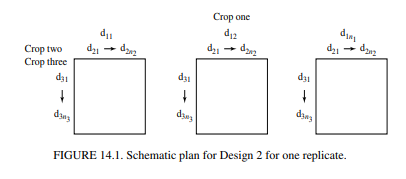
A procedure for reducing the number of entries and the space requirements would be to utilize the ideas of Federer and Scully (1993) in the manner shown in Figure $14.1$, using the previous example for three crops. There are $n_{1}$ experimental units in each replicate; the density for crop two varies from the lowest to the highest density horizontally either continuously increasing or increasing by increments; and the crop three densities vary in the same way but vertically, with highest combined densities being in the lower right-hand corner of an experimental unit. The experimenter would divide each experimental unit into $n_{2} n_{3}$ equal-sized rectangles and obtain the response for each of these rectangles. The density level for each rectangle would be the average density in that rectangle. The $n_{1}$ experimental units are randomly allocated in each replicate in the experiment and the crop two and crop three densities are systematically increasing within the experimental unit. Thus, the crop one density levels are somewhat akin to a “whole plot” and the density levels of crops two and three are somewhat like “split plots.” A response function, e.g., a second-degree polynomial, would be fitted, the maximum value on the response surface, and/or the area under the response function could be used as the response for the experimental unit (see Federer and Scully, 1993). The selection of which crop to use as crop one is important, but probably one crop would be an obvious candidate. For the first example above, cassava would be crop one because a large experimental unit relative to the one needed for maize or beans would be required. In other situations, one of the crops may utilize well-defined discrete levels and, hence, would be a candidate to be crop one. There should be no gradients within each of the experimental units in order that a gradient effect does not become confounded with the effect of density level on the response.
实验设计与分析代写
统计代写|实验设计与分析作业代写Design and Analysis of Experiments代考|All Crops in a Mixture
第 12 章考虑了混合中三种或多种作物以及一种主要作物和两种或多种次要作物间作的最简单形式。与第一卷第 2 章(两种作物)中的统计分析相比,统计分析的复杂性有所增加. 第 1 卷第 3 章和第 4 章的方法在第 13 章中扩展到三种或更多作物的混合物。介绍了每种作物的单个作物响应分析以及混合物中所有作物的组合响应分析。混合物中给定作物的密度在混合物之间保持恒定。在本章中,考虑了允许部分或所有作物具有不同密度的种植系统。本文介绍的方法是第一卷第 5 章中介绍的方法的概括。
混合物中不同和/或恒定密度的许多图案都是可能的。选择用于研究的特定密度将取决于作物混合物的组成以及实验的目标。对于一种主要作物和两种或多种次要作物:
(i) 主要作物的密度可以变化,而次要作物的密度保持不变。
(ii) 主要作物的密度可以保持不变,而次要作物的部分或全部密度可以变化。
(iii) 混合物中所有作物的密度可以变化。
三种或三种以上主要作物和一些或没有次要作物混合在一起,可能会出现以下情况:
78
- 改变混合物中某些或所有作物
的密度 (i) 混合物中所有主要作物的密度可以改变。
(ii) 两种或多种主要作物的密度可以保持不变,而其余作物的密度可以变化。
(iii) (i) 或 (ii) 中包括的任何次要作物的密度可以变化或保持不变。 - 正如第一卷第 5 章所讨论的,需要认真注意为每种作物选择不同的密度水平。实验者需要决定是否使为一种作物选择的水平依赖于或独立于为混合物中的其余作物选择的水平。接近混合物中所有作物的最大密度可能是有意义的,因为无论作物如何,植物的总数是总人口水平,超过该水平就不会增加产量。水分、植物养分、阳光等的量可能决定了一块土地上可以支持的最大人口水平。众所周知,人口过剩会导致产量减少甚至为零。为了确定产生最大或接近最大响应的密度水平,建议选择的电平略高于给出最大响应的电平。例如,玉米的最大产量可以达到每公顷 60,000 株。每公顷 70,000 株甚至 80,000 株植物的水平应该会导致产量下降,并且应该包括在实验中进行研究。在确定响应曲线时,实验者经常犯的错误是只包括“将在实践中使用”的水平。包含超出实践中通常使用的水平的水平会导致更准确的响应曲线显示响应和密度水平之间的关系。如果响应曲线在最高密度处未显示下降,则不清楚是否已达到最大值以及是否应包括更高的密度水平。玉米的最高产量可以达到每公顷 60,000 株。每公顷 70,000 株甚至 80,000 株植物的水平应该会导致产量下降,并且应该包括在实验中进行研究。在确定响应曲线时,实验者经常犯的错误是只包括“将在实践中使用”的水平。包含超出实践中通常使用的水平的水平会导致更准确的响应曲线显示响应和密度水平之间的关系。如果响应曲线在最高密度处未显示下降,则不清楚是否已达到最大值以及是否应包括更高的密度水平。玉米的最高产量可以达到每公顷 60,000 株。每公顷 70,000 株甚至 80,000 株植物的水平应该会导致产量下降,并且应该包括在实验中进行研究。在确定响应曲线时,实验者经常犯的错误是只包括“将在实践中使用”的水平。包含超出实践中通常使用的水平的水平会导致更准确的响应曲线显示响应和密度水平之间的关系。如果响应曲线在最高密度处未显示下降,则不清楚是否已达到最大值以及是否应包括更高的密度水平。每公顷植物应导致产量下降,并应包括在实验中进行研究。在确定响应曲线时,实验者经常犯的错误是只包括“将在实践中使用”的水平。包含超出实践中通常使用的水平的水平会导致更准确的响应曲线显示响应和密度水平之间的关系。如果响应曲线在最高密度处未显示下降,则不清楚是否已达到最大值以及是否应包括更高的密度水平。每公顷植物应导致产量下降,并应包括在实验中进行研究。在确定响应曲线时,实验者经常犯的错误是只包括“将在实践中使用”的水平。包含超出实践中通常使用的水平的水平会导致更准确的响应曲线显示响应和密度水平之间的关系。如果响应曲线在最高密度处未显示下降,则不清楚是否已达到最大值以及是否应包括更高的密度水平。” 包含超出实践中通常使用的水平会导致更准确的响应曲线显示响应和密度水平之间的关系。如果响应曲线在最高密度处未显示下降,则不清楚是否已达到最大值以及是否应包括更高的密度水平。” 包含超出实践中通常使用的水平会导致更准确的响应曲线显示响应和密度水平之间的关系。如果响应曲线在最高密度处未显示下降,则不清楚是否已达到最大值以及是否应包括更高的密度水平。
统计代写|实验设计与分析作业代写Design and Analysis of Experiments代考|Treatment Design
几种处理设计可用于研究混合物中作物不同密度水平的反应。我们将列出一些用于研究产量-密度关系的可能设计。
考虑三种作物的混合密度0<d一世1<d一世2<⋯<d一世n一世农作物一世在n一世密度水平。那么,对于n1=3,n2=2, 和n3=4,获得以下组合(标记为 X),例如,作物一是木薯,作物二是豆类,作物三是玉米:除了上述 24 种组合外,还可以包括作为单一作物的 3 种作物以获得(3×2×4)+(3+2+4)=33条目。这里密度最低d一世1,一世=1,2和 3 均大于零。随着作物密度水平的数量和作物数量的增加,实验的条目总数迅速增加。例如,在上述集合中包含三个密度级别的第四种作物将导致(3×2×4×3)+(3+2+4+3)=84条目。因此,实验者在选择精确的水平及其数量时需要非常小心,以使条目的数量不会超出实验所能完成的范围。该处理设计包含所有可能的密度水平组合以及每种单一作物的水平。
统计代写|实验设计与分析作业代写Design and Analysis of Experiments代考|A procedure for reducing
减少条目数量和空间要求的程序是利用 Federer 和 Scully (1993) 的思想,如图 1 所示。14.1,将前面的示例用于三种作物。有n1每个重复中的实验单元;作物二的密度从最低到最高水平水平变化,连续增加或增量增加;作物的三种密度以相同的方式变化,但垂直变化,最高的组合密度位于实验单元的右下角。实验者将每个实验单元分成n2n3大小相等的矩形并获得每个矩形的响应。每个矩形的密度级别将是该矩形的平均密度。这n1实验单元在实验的每个重复中随机分配,并且作物二和作物三的密度在实验单元内系统地增加。因此,作物一的密度水平有点类似于“整块地”,而作物二和三的密度水平有点像“裂地”。将拟合响应函数,例如二次多项式,响应曲面上的最大值和/或响应函数下的区域可用作实验单元的响应(参见 Federer 和 Scully,1993 )。选择哪一种作物作为第一作物很重要,但很可能一种作物是一个明显的候选者。对于上面的第一个示例,木薯将是一种作物,因为相对于玉米或豆类所需的实验单位而言,需要一个大的实验单位。在其他情况下,其中一种作物可能利用明确定义的离散水平,因此将成为作物之一的候选者。每个实验单元内不应有梯度,以免梯度效应与密度水平对响应的影响相混淆。

统计代写请认准statistics-lab™. statistics-lab™为您的留学生涯保驾护航。统计代写|python代写代考
随机过程代考
在概率论概念中,随机过程是随机变量的集合。 若一随机系统的样本点是随机函数,则称此函数为样本函数,这一随机系统全部样本函数的集合是一个随机过程。 实际应用中,样本函数的一般定义在时间域或者空间域。 随机过程的实例如股票和汇率的波动、语音信号、视频信号、体温的变化,随机运动如布朗运动、随机徘徊等等。
贝叶斯方法代考
贝叶斯统计概念及数据分析表示使用概率陈述回答有关未知参数的研究问题以及统计范式。后验分布包括关于参数的先验分布,和基于观测数据提供关于参数的信息似然模型。根据选择的先验分布和似然模型,后验分布可以解析或近似,例如,马尔科夫链蒙特卡罗 (MCMC) 方法之一。贝叶斯统计概念及数据分析使用后验分布来形成模型参数的各种摘要,包括点估计,如后验平均值、中位数、百分位数和称为可信区间的区间估计。此外,所有关于模型参数的统计检验都可以表示为基于估计后验分布的概率报表。
广义线性模型代考
广义线性模型(GLM)归属统计学领域,是一种应用灵活的线性回归模型。该模型允许因变量的偏差分布有除了正态分布之外的其它分布。
statistics-lab作为专业的留学生服务机构,多年来已为美国、英国、加拿大、澳洲等留学热门地的学生提供专业的学术服务,包括但不限于Essay代写,Assignment代写,Dissertation代写,Report代写,小组作业代写,Proposal代写,Paper代写,Presentation代写,计算机作业代写,论文修改和润色,网课代做,exam代考等等。写作范围涵盖高中,本科,研究生等海外留学全阶段,辐射金融,经济学,会计学,审计学,管理学等全球99%专业科目。写作团队既有专业英语母语作者,也有海外名校硕博留学生,每位写作老师都拥有过硬的语言能力,专业的学科背景和学术写作经验。我们承诺100%原创,100%专业,100%准时,100%满意。
机器学习代写
随着AI的大潮到来,Machine Learning逐渐成为一个新的学习热点。同时与传统CS相比,Machine Learning在其他领域也有着广泛的应用,因此这门学科成为不仅折磨CS专业同学的“小恶魔”,也是折磨生物、化学、统计等其他学科留学生的“大魔王”。学习Machine learning的一大绊脚石在于使用语言众多,跨学科范围广,所以学习起来尤其困难。但是不管你在学习Machine Learning时遇到任何难题,StudyGate专业导师团队都能为你轻松解决。
多元统计分析代考
基础数据: $N$ 个样本, $P$ 个变量数的单样本,组成的横列的数据表
变量定性: 分类和顺序;变量定量:数值
数学公式的角度分为: 因变量与自变量
时间序列分析代写
随机过程,是依赖于参数的一组随机变量的全体,参数通常是时间。 随机变量是随机现象的数量表现,其时间序列是一组按照时间发生先后顺序进行排列的数据点序列。通常一组时间序列的时间间隔为一恒定值(如1秒,5分钟,12小时,7天,1年),因此时间序列可以作为离散时间数据进行分析处理。研究时间序列数据的意义在于现实中,往往需要研究某个事物其随时间发展变化的规律。这就需要通过研究该事物过去发展的历史记录,以得到其自身发展的规律。
回归分析代写
多元回归分析渐进(Multiple Regression Analysis Asymptotics)属于计量经济学领域,主要是一种数学上的统计分析方法,可以分析复杂情况下各影响因素的数学关系,在自然科学、社会和经济学等多个领域内应用广泛。
MATLAB代写
MATLAB 是一种用于技术计算的高性能语言。它将计算、可视化和编程集成在一个易于使用的环境中,其中问题和解决方案以熟悉的数学符号表示。典型用途包括:数学和计算算法开发建模、仿真和原型制作数据分析、探索和可视化科学和工程图形应用程序开发,包括图形用户界面构建MATLAB 是一个交互式系统,其基本数据元素是一个不需要维度的数组。这使您可以解决许多技术计算问题,尤其是那些具有矩阵和向量公式的问题,而只需用 C 或 Fortran 等标量非交互式语言编写程序所需的时间的一小部分。MATLAB 名称代表矩阵实验室。MATLAB 最初的编写目的是提供对由 LINPACK 和 EISPACK 项目开发的矩阵软件的轻松访问,这两个项目共同代表了矩阵计算软件的最新技术。MATLAB 经过多年的发展,得到了许多用户的投入。在大学环境中,它是数学、工程和科学入门和高级课程的标准教学工具。在工业领域,MATLAB 是高效研究、开发和分析的首选工具。MATLAB 具有一系列称为工具箱的特定于应用程序的解决方案。对于大多数 MATLAB 用户来说非常重要,工具箱允许您学习和应用专业技术。工具箱是 MATLAB 函数(M 文件)的综合集合,可扩展 MATLAB 环境以解决特定类别的问题。可用工具箱的领域包括信号处理、控制系统、神经网络、模糊逻辑、小波、仿真等。