标签: BMS14

统计代写|实验设计与分析作业代写Design and Analysis of Experiments代考| Statistical Analyses for Sole Crop Respons

如果你也在 怎样代写实验设计与分析Design and Analysis of Experiments这个学科遇到相关的难题,请随时右上角联系我们的24/7代写客服。

实验设计与分析提供了一个严格的介绍,通过质量和性能优化来改进产品和工艺设计。

statistics-lab™ 为您的留学生涯保驾护航 在代写实验设计与分析Design and Analysis of Experiments方面已经树立了自己的口碑, 保证靠谱, 高质且原创的统计Statistics代写服务。我们的专家在代写实验设计与分析Design and Analysis of Experiments方面经验极为丰富,各种代写实验设计与分析Design and Analysis of Experiments相关的作业也就用不着说。

我们提供的实验设计与分析Design and Analysis of Experiments及其相关学科的代写,服务范围广, 其中包括但不限于:

  • Statistical Inference 统计推断
  • Statistical Computing 统计计算
  • Advanced Probability Theory 高等楖率论
  • Advanced Mathematical Statistics 高等数理统计学
  • (Generalized) Linear Models 广义线性模型
  • Statistical Machine Learning 统计机器学习
  • Longitudinal Data Analysis 纵向数据分析
  • Foundations of Data Science 数据科学基础
统计代写|实验设计与分析作业代写Design and Analysis of Experiments代考| Statistical Analyses for Sole Crop Respons

统计代写|实验设计与分析作业代写Design and Analysis of Experiments代考|Statistical Analyses for Sole Crop Respons

For crop $h$ in a mixture of $c$ crops in Design 1 and for the $v$ entries arranged in a randomized complete block experiment design of $r$ complete blocks, let the response equation, for crop $h=1$ say, be of the usual form:
$$
Y_{g d_{\mathrm{H}}\left(d_{2 i} d_{\left.3_{j} \cdots\right)}\right.}=\mu+\rho_{g}+\tau_{d_{4 i}\left(d_{2 i} d_{j \cdots} \cdots\right)}+\epsilon_{g d_{1 i}\left(d_{2 i} d_{3 i}\right)},
$$
where $\mu$ is a general mean effect, $\rho_{g}$ is the $g$ th complete block effect, $\tau_{d_{1 i}\left(d_{2} d_{3 j} \cdots\right)}$ is the effect of the $d_{1 i}\left(d_{2 i} d_{3 i} \cdots\right)$ th combination from the $n_{1} \times n_{2} \times n_{3} \times \cdots \mathrm{com}-$ binations of the density levels $d_{1 i}, d_{2 i}, d_{3 i}, \ldots, i=1,2, \ldots, n_{h}, h=1,2, \ldots, c$, the number of crops in a mixture, and the $\epsilon_{g d_{1 i}\left(d_{2} d_{3} \ldots\right)}$ are random error terms distributed with zero mean and variance $\sigma_{e h}^{2}$. An analysis of variance (ANOVA) for this situation is given in Table $14.1$ for the case when the lowest density level is not zero. The sums of squares are computed in the usual manner for a factorial treatment design in a randomized complete block experiment design.

If desired, each of the treatment sums of squares could be partitioned into single degree of freedom contrasts such as linear, quadratic, etc., or some other set of

contrasts dependent on the particular response function used for the relationship between a response such as yield and density level.

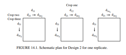
A response function of the following nature might be suitable for the $n_{2} n_{3}$ responses obtained on a single experimental unit $g d_{1 h}$ from Design 2 :
$$
\begin{aligned}
Y_{i j}=& \alpha+\beta_{1} d_{2 i}+\beta_{2} d_{2 i}^{2}+\beta_{3} d_{3 j}+\beta_{4} d_{3 j}^{2}+\beta_{5} d_{2 i} d_{3 j} \
&+\beta_{6} d_{2 i} d_{3 j}^{2}+\beta_{7} d_{2 i}^{2} d_{3 j}+\epsilon_{i j},
\end{aligned}
$$
where $i=1, \ldots, n_{2}, j=1, \ldots, n_{3}, h=1, \ldots, n_{1}$, the $\beta$ ‘s are polynomial regression coefficients, and the $d_{2 i}$ and $d_{3 j}$ are the various density levels for crops two and three. Of course, other response functions may be more appropriate than the above one. However, this particular model does allow for linear and curvilinear responses for each crop as well as for some rather well-behaved interaction terms. The responses used would be the predicted values from the above regression equation. This response model equation may also be used for each of the $n_{1} n_{2}$ experimental units from Design 3. The main object of this analysis is to show the effect of changing levels of the densities of crops two and three at each level of crop one. An alternate analysis would be a MANOVA (multivariate analysis of variance) or discriminant function analysis, using the seven regression coefficients as the seven variates and determining their effects over all levels of crop one. Still another analysis would be to obtain the estimated maximum responses from the regression function in equation (14.2) in each of the $r n_{1}$ experimental units and perform an analysis on these values.

统计代写|实验设计与分析作业代写Design and Analysis of Experiments代考|Statistical Analyses

Using these created variables, ANOVAs like those given above can be obtained. Such analyses as these are more useful than those in the previous section, as they deal with the system of intercropping rather than concentrating on the components, individual crops, of the system.

Other analyses such as AMMI (additive main effects and multiplicative interaction; see Gauch, 1988, Gauch and Zobel, 1988, Ezumah et al., 1991, and related references) and MANOVA (multivariate analysis of variance, see Chapter 4 of Volume I, e.g.) may be useful in certain cases. For these analyses, the responses for the individual crops form the variates for the multivariate analyses, and functionals combining response from all crops would be obtained. The interpretation of the resulting principle components and canonical variates may be a problem. These statistics may differ if a logarithmic or some other transformation of the responses had been made before using AMMI or MANOVA. Hence, selective and careful use of these procedures are necessary in order for them to be of practical and interpretive usefulness for a researcher. In some cases, little, if anything new, is added by these more complex procedures (see, e.g., Ezumah et al., 1991). For many situations using analyses involving the created variables in (i), (ii), (iii), and (iv) above will suffice. In some cases, other functionals such as AMMI and MANOVA may be useful.

统计代写|实验设计与分析作业代写Design and Analysis of Experiments代考|Modeling Responses in Sole Crop Yields

Many yield-density or response-density relationships can be formulated [see Section 3 of Morales (1993) and references therein]. In order not to make the modeling process too complicated, we shall consider simple relationships. A simple model is a linear relation between yield and density. For a randomized complete block design with three sole crops, say cassava $=c$, maize $=m$, and beans $=b$, the

response models are
$$
\begin{aligned}
&Y_{g c h}=\mu_{c c}+\rho_{g c}+\beta_{1 c}\left(d_{c h}-\bar{d}{c}\right)+\epsilon{g c h}=\beta_{0 g c}+\beta_{1 c} d_{c h}+\epsilon_{g c h}, \
&Y_{g m i}=\beta_{0 g m}+\beta_{1 m} d_{m i}+\epsilon_{g m i} \text {, } \
&Y_{g b j}=\beta_{0 g b}+\beta_{1 b} d_{b j}+\epsilon_{g b j} .
\end{aligned}
$$

$$
\hat{\beta}{1 m}=\sum{i=1}^{n_{m}}\left(d_{m i}-\bar{d}{m}\right)\left(\bar{y}{m i}-\bar{y}{m m}\right) / \sum{i=1}^{n_{m}}\left(d_{m i}-\bar{d}{m \cdot}\right)^{2} $$ 14.6 Modeling Responses for Mixtures Based on Sole Crop Model 89 $$ \hat{\beta}{1 b}=\sum_{j=1}^{n_{b}}\left(d_{b j}-\bar{d}{b .}\right)\left(\bar{y}{b j}-\bar{y}{b .}\right) / \sum{j=1}^{n_{b}}\left(d_{b j}-\bar{d}{b .}\right)^{2}, $$ where the $\bar{y}$ and $\bar{d}$ are mean values for the corresponding values of responses and densities, respectively, and $\beta{0 c}, \beta_{0 \mathrm{~m}}$, and $\beta_{0 b}$ are the intercepts averaged over replicates. Extension of the above to $c$ more than 3 crops is straightforward. The above assumes that density levels are the same from replicate to replicate. If this is not the true situation, e.g., missing plots occur, the above formulas will need to be adjusted to account for the change in density levels.

In the event that monocrop responses are not available, it is possible to model yield-density relationships using the lowest density levels for all other crops but the one under consideration. For example, this relationship for crop one, say, is obtained from the responses at levels $d_{21} d_{31} \cdots$ for crops two, three, etc. Using the above cassava-maize-bean example, the yield-density models would be
$$
\begin{aligned}
&Y_{g d_{c t h}\left(d_{m 1} d_{b 1}\right)}=\beta_{g} 0 c+\beta_{1 c} d_{c h}+\epsilon_{g d_{c h}\left(d_{m 1} d_{b 1}\right)}, \
&Y_{g d_{m i}\left(d_{c 1} d_{b 1}\right)}=\beta_{g 0 m}+\beta_{1 m} d_{m i}+\epsilon_{g d_{m i} i}\left(d_{c 1} d_{b 1}\right), \
&\left.Y_{g d_{b j}\left(d_{c 1} d_{m 1}\right.}\right)=\beta_{g 0 b}+\beta_{1 b} d_{b j}+\epsilon_{g d_{b j}\left(d_{c t} d_{m 1}\right)},
\end{aligned}
$$
where $g d_{c h 1}\left(d_{m 1} d_{b 1}\right)$ is for level $d_{c h}$ at levels $d_{m 1}$ and $d_{b 1}$ in replicate $g$ and where the regression coefficients are defined in a manner similar to that for equations (14.3)(14.5). The least squares solutions for the parameters of (14.18)-(14.20) are much the same as given in equations (14.6)-(14.17). Because of the direct application of the above solution with the necessary changes to account for computing the regressions on the lowest-density levels of all crops but the one in question, the least squares solutions are not given, as they are straightforward.

统计代写|实验设计与分析作业代写Design and Analysis of Experiments代考| Statistical Analyses for Sole Crop Respons

实验设计与分析代写

统计代写|实验设计与分析作业代写Design and Analysis of Experiments代考|Statistical Analyses for Sole Crop Respons

对于作物H在混合C设计 1 中的作物和v条目排列在随机完整区组实验设计中r完整的块,让响应方程,用于作物H=1比如说,采用通常的形式:
是GdH(d2一世d3j⋯)=μ+ρG+τd4一世(d2一世dj⋯⋯)+εGd1一世(d2一世d3一世),
在哪里μ是一般平均效应,ρG是个G完整的方块效果,τd1一世(d2d3j⋯)是的效果d1一世(d2一世d3一世⋯)来自的组合n1×n2×n3×⋯C这米−密度级别的组合d1一世,d2一世,d3一世,…,一世=1,2,…,nH,H=1,2,…,C,混合物中的作物数量,以及εGd1一世(d2d3…)是零均值和方差分布的随机误差项σ和H2. 表中给出了这种情况的方差分析 (ANOVA)14.1对于最低密度水平不为零的情况。平方和的计算方式与随机完全区组试验设计中的因子处理设计相同。

如果需要,可以将每个处理平方和划分为单个自由度对比,例如线性、二次等,或其他一些组

对比取决于用于响应之间关系的特定响应函数,例如产量和密度水平。

以下性质的响应函数可能适用于n2n3在单个实验单元上获得的响应Gd1H来自设计 2:
是一世j=一种+b1d2一世+b2d2一世2+b3d3j+b4d3j2+b5d2一世d3j +b6d2一世d3j2+b7d2一世2d3j+ε一世j,
在哪里一世=1,…,n2,j=1,…,n3,H=1,…,n1, 这b是多项式回归系数,并且d2一世和d3j是作物二和三的不同密度水平。当然,其他响应函数可能比上述函数更合适。然而,这个特定的模型确实允许每种作物的线性和曲线响应以及一些表现良好的交互项。使用的响应将是来自上述回归方程的预测值。该响应模型方程也可用于每个n1n2来自设计 3 的实验单元。该分析的主要目的是显示在作物 1 的每个水平上改变作物 2 和 3 的密度水平的影响。另一种分析是 MANOVA(多变量方差分析)或判别函数分析,使用七个回归系数作为七个变量,并确定它们对作物一的所有水平的影响。还有一种分析是从方程(14.2)中的回归函数获得估计的最大响应,在每个rn1实验单元并对这些值进行分析。

统计代写|实验设计与分析作业代写Design and Analysis of Experiments代考|Statistical Analyses

使用这些创建的变量,可以获得像上面给出的 ANOVA。这些分析比上一节中的分析更有用,因为它们处理的是间作系统,而不是集中于系统的组成部分、单个作物。

其他分析,如 AMMI(加性主效应和乘法交互;参见 Gauch,1988,Gauch 和 Zobel,1988,Ezumah 等人,1991 和相关参考资料)和 MANOVA(多变量方差分析,参见第一卷第 4 章,例如)在某些情况下可能有用。对于这些分析,单个作物的响应形成多变量分析的变量,并且将获得结合所有作物响应的泛函。由此产生的主成分和规范变量的解释可能是一个问题。如果在使用 AMMI 或 MANOVA 之前对响应进行了对数或其他一些转换,这些统计数据可能会有所不同。因此,有必要选择性和谨慎地使用这些程序,以使它们对研究人员具有实用性和解释性。在某些情况下,这些更复杂的程序几乎没有添加任何新内容(例如,参见 Ezumah 等人,1991)。对于许多情况,使用涉及上述 (i)、(ii)、(iii) 和 (iv) 中创建的变量的分析就足够了。在某些情况下,其他函数(例如 AMMI 和 MANOVA)可能有用。

统计代写|实验设计与分析作业代写Design and Analysis of Experiments代考|Modeling Responses in Sole Crop Yields

许多产量-密度或响应-密度关系可以被制定[见 Morales (1993) 的第 3 节和其中的参考资料]。为了不使建模过程过于复杂,我们将考虑简单的关系。一个简单的模型是产量和密度之间的线性关系。对于具有三种单一作物的随机完整区组设计,例如木薯=C, 玉米=米, 和豆子=b, 这

响应模型是
是GCH=μCC+ρGC+b1C(dCH−d¯C)+εGCH=b0GC+b1CdCH+εGCH, 是G米一世=b0G米+b1米d米一世+εG米一世,  是Gbj=b0Gb+b1bdbj+εGbj.b^1米=∑一世=1n米(d米一世−d¯米)(是¯米一世−是¯米米)/∑一世=1n米(d米一世−d¯米⋅)214.6 基于单一作物模型的混合物响应建模 89b^1b=∑j=1nb(dbj−d¯b.)(是¯bj−是¯b.)/∑j=1nb(dbj−d¯b.)2,在哪里是¯和d¯分别是响应和密度的相应值的平均值,和b0C,b0 米, 和b0b是重复次数的平均截距。将上述扩展为C超过 3 种作物是直截了当的。以上假设密度水平从复制到复制是相同的。如果这不是真实情况,例如出现缺失图,则需要调整上述公式以考虑密度水平的变化。

如果无法获得单一作物的响应,则可以使用除正在考虑的作物之外的所有其他作物的最低密度水平来模拟产量-密度关系。例如,作物一的这种关系,例如,是从水平的响应中获得的d21d31⋯对于作物二、三等。使用上面的木薯玉米豆示例,产量密度模型将是
是GdC吨H(d米1db1)=bG0C+b1CdCH+εGdCH(d米1db1), 是Gd米一世(dC1db1)=bG0米+b1米d米一世+εGd米一世一世(dC1db1), 是Gdbj(dC1d米1)=bG0b+b1bdbj+εGdbj(dC吨d米1),
在哪里GdCH1(d米1db1)是为了水平dCH在级别d米1和db1复制中G其中回归系数的定义方式类似于方程 (14.3)(14.5)。(14.18)-(14.20) 的参数的最小二乘解与方程 (14.6)-(14.17) 中给出的大致相同。由于直接应用上述解决方案并进行必要的更改以计算除所讨论的所有作物的最低密度水平的回归,因此没有给出最小二乘解决方案,因为它们很简单。

统计代写|实验设计与分析作业代写Design and Analysis of Experiments代考 请认准statistics-lab™

统计代写请认准statistics-lab™. statistics-lab™为您的留学生涯保驾护航。统计代写|python代写代考

随机过程代考

在概率论概念中,随机过程随机变量的集合。 若一随机系统的样本点是随机函数,则称此函数为样本函数,这一随机系统全部样本函数的集合是一个随机过程。 实际应用中,样本函数的一般定义在时间域或者空间域。 随机过程的实例如股票和汇率的波动、语音信号、视频信号、体温的变化,随机运动如布朗运动、随机徘徊等等。

贝叶斯方法代考

贝叶斯统计概念及数据分析表示使用概率陈述回答有关未知参数的研究问题以及统计范式。后验分布包括关于参数的先验分布,和基于观测数据提供关于参数的信息似然模型。根据选择的先验分布和似然模型,后验分布可以解析或近似,例如,马尔科夫链蒙特卡罗 (MCMC) 方法之一。贝叶斯统计概念及数据分析使用后验分布来形成模型参数的各种摘要,包括点估计,如后验平均值、中位数、百分位数和称为可信区间的区间估计。此外,所有关于模型参数的统计检验都可以表示为基于估计后验分布的概率报表。

广义线性模型代考

广义线性模型(GLM)归属统计学领域,是一种应用灵活的线性回归模型。该模型允许因变量的偏差分布有除了正态分布之外的其它分布。

statistics-lab作为专业的留学生服务机构,多年来已为美国、英国、加拿大、澳洲等留学热门地的学生提供专业的学术服务,包括但不限于Essay代写,Assignment代写,Dissertation代写,Report代写,小组作业代写,Proposal代写,Paper代写,Presentation代写,计算机作业代写,论文修改和润色,网课代做,exam代考等等。写作范围涵盖高中,本科,研究生等海外留学全阶段,辐射金融,经济学,会计学,审计学,管理学等全球99%专业科目。写作团队既有专业英语母语作者,也有海外名校硕博留学生,每位写作老师都拥有过硬的语言能力,专业的学科背景和学术写作经验。我们承诺100%原创,100%专业,100%准时,100%满意。

机器学习代写

随着AI的大潮到来,Machine Learning逐渐成为一个新的学习热点。同时与传统CS相比,Machine Learning在其他领域也有着广泛的应用,因此这门学科成为不仅折磨CS专业同学的“小恶魔”,也是折磨生物、化学、统计等其他学科留学生的“大魔王”。学习Machine learning的一大绊脚石在于使用语言众多,跨学科范围广,所以学习起来尤其困难。但是不管你在学习Machine Learning时遇到任何难题,StudyGate专业导师团队都能为你轻松解决。

多元统计分析代考


基础数据: $N$ 个样本, $P$ 个变量数的单样本,组成的横列的数据表
变量定性: 分类和顺序;变量定量:数值
数学公式的角度分为: 因变量与自变量

时间序列分析代写

随机过程,是依赖于参数的一组随机变量的全体,参数通常是时间。 随机变量是随机现象的数量表现,其时间序列是一组按照时间发生先后顺序进行排列的数据点序列。通常一组时间序列的时间间隔为一恒定值(如1秒,5分钟,12小时,7天,1年),因此时间序列可以作为离散时间数据进行分析处理。研究时间序列数据的意义在于现实中,往往需要研究某个事物其随时间发展变化的规律。这就需要通过研究该事物过去发展的历史记录,以得到其自身发展的规律。

回归分析代写

多元回归分析渐进(Multiple Regression Analysis Asymptotics)属于计量经济学领域,主要是一种数学上的统计分析方法,可以分析复杂情况下各影响因素的数学关系,在自然科学、社会和经济学等多个领域内应用广泛。

MATLAB代写

MATLAB 是一种用于技术计算的高性能语言。它将计算、可视化和编程集成在一个易于使用的环境中,其中问题和解决方案以熟悉的数学符号表示。典型用途包括:数学和计算算法开发建模、仿真和原型制作数据分析、探索和可视化科学和工程图形应用程序开发,包括图形用户界面构建MATLAB 是一个交互式系统,其基本数据元素是一个不需要维度的数组。这使您可以解决许多技术计算问题,尤其是那些具有矩阵和向量公式的问题,而只需用 C 或 Fortran 等标量非交互式语言编写程序所需的时间的一小部分。MATLAB 名称代表矩阵实验室。MATLAB 最初的编写目的是提供对由 LINPACK 和 EISPACK 项目开发的矩阵软件的轻松访问,这两个项目共同代表了矩阵计算软件的最新技术。MATLAB 经过多年的发展,得到了许多用户的投入。在大学环境中,它是数学、工程和科学入门和高级课程的标准教学工具。在工业领域,MATLAB 是高效研究、开发和分析的首选工具。MATLAB 具有一系列称为工具箱的特定于应用程序的解决方案。对于大多数 MATLAB 用户来说非常重要,工具箱允许您学习应用专业技术。工具箱是 MATLAB 函数(M 文件)的综合集合,可扩展 MATLAB 环境以解决特定类别的问题。可用工具箱的领域包括信号处理、控制系统、神经网络、模糊逻辑、小波、仿真等。

R语言代写问卷设计与分析代写
PYTHON代写回归分析与线性模型代写
MATLAB代写方差分析与试验设计代写
STATA代写机器学习/统计学习代写
SPSS代写计量经济学代写
EVIEWS代写时间序列分析代写
EXCEL代写深度学习代写
SQL代写各种数据建模与可视化代写

统计代写|实验设计与分析作业代写Design and Analysis of Experiments代考| Varying Densities for Some

如果你也在 怎样代写实验设计与分析Design and Analysis of Experiments这个学科遇到相关的难题,请随时右上角联系我们的24/7代写客服。

实验设计与分析提供了一个严格的介绍,通过质量和性能优化来改进产品和工艺设计。

statistics-lab™ 为您的留学生涯保驾护航 在代写实验设计与分析Design and Analysis of Experiments方面已经树立了自己的口碑, 保证靠谱, 高质且原创的统计Statistics代写服务。我们的专家在代写实验设计与分析Design and Analysis of Experiments方面经验极为丰富,各种代写实验设计与分析Design and Analysis of Experiments相关的作业也就用不着说。

我们提供的实验设计与分析Design and Analysis of Experiments及其相关学科的代写,服务范围广, 其中包括但不限于:

  • Statistical Inference 统计推断
  • Statistical Computing 统计计算
  • Advanced Probability Theory 高等楖率论
  • Advanced Mathematical Statistics 高等数理统计学
  • (Generalized) Linear Models 广义线性模型
  • Statistical Machine Learning 统计机器学习
  • Longitudinal Data Analysis 纵向数据分析
  • Foundations of Data Science 数据科学基础
统计代写|实验设计与分析作业代写Design and Analysis of Experiments代考| Varying Densities for Some

统计代写|实验设计与分析作业代写Design and Analysis of Experiments代考|All Crops in a Mixture

The simplest form of intercropping with three or more crops in the mixture and with one major crop and two or more minor crops was considered in Chapter 12. The complexity of the statistical analyses over that in Chapter 2 (two crops) of Volume I is increased. The methods of Chapters 3 and 4 of Volume I were extended to mixtures of three or more crops in Chapter 13. Analyses for individual crop responses for each crop as well as analyses for combined responses for all crops in the mixture are presented. The density for a given crop in the mixture was held constant from mixture to mixture. In the present chapter, cropping systems which allow varying densities for some or all crops are considered. The methods presented herein are a generalization of those presented in Chapter 5 of Volume I.
Many patterns for varying and/or constant densities in a mixture are possible. The particular densities selected for study will depend on the makeup of the crop mixture as well as the goals of the experiment. With one major crop and two or more minor crops:
(i) The density of the major crop could be varied and the densities of the minor crops kept constant.
(ii) The density of the major crop could be held constant and some or all of the densities of the minor crops varied.
(iii) The densities of all crops in the mixture could be varied.
With three or more major crops and with some or no minor crops in a mixture, the following situations are possible:
78

  1. Varying Densities for Some or All Crops in a Mixture
    (i) The densities of all major crops in the mixture could be varied.
    (ii) The densities of two or more major crops could be constant and the densities of the remaining crops could be varied.
    (iii) The densities of any minor crops included in (i) or (ii) could be varied or held constant.
  2. As discussed in Chapter 5 of Volume I, serious attention needs to be given to selecting the various density levels for each crop. The experimenter needs to decide whether to make the levels selected for one crop dependent or independent of the levels selected for the remaining crops in a mixture. It may make sense to approach a maximum density for all crops in the mixture as the total number of plants, regardless of crop, is the total population level beyond which there will be no increased yields. The amount of moisture, plant nutrients, sunlight, etc. may dictate the maximum population level that can be supported on a plot of ground. It is well known that overpopulation can result in reduced or even zero yields. In order to pinpoint density levels producing maximum or nearmaximum responses, it is advisable to select levels somewhat beyond the level giving maximum response. For example, the maximum yield of maize may be attained with 60,000 plants per hectare. A level of 70,000 , or even 80,000 , plants per hectare should result in decreased yields and should be included for study in an experiment. In determining response curves, experimenters often make the mistake of including only levels which “would be used in practice.” The inclusion of levels beyond those normally used in practice results in a more accurate response curve showing the relationship between response and density level. If a response curve does not show a decrease at the highest density, it is not clear that the maximum has been attained and that higher density levels should have been included.

统计代写|实验设计与分析作业代写Design and Analysis of Experiments代考|Treatment Design

Several treatment designs may be used for studying responses over varying density levels of the crops in the mixture. We shall list some of the possible designs for studying yield-density relationships.

Consider a mixture of three crops at densities $0<d_{i 1}<d_{i 2}<\cdots<d_{i n_{i}}$ for crop $i$ at $n_{i}$ density levels. Then, for $n_{1}=3, n_{2}=2$, and $n_{3}=4$, the following combinations (marked X) are obtained where, for example, crop one is cassava, crop two is beans, and crop three is maize:In addition to the above 24 combinations, the 3 crops as sole crops could be included to obtain $(3 \times 2 \times 4)+(3+2+4)=33$ entries. Here the lowest densities $d_{i 1}, i=1,2$, and 3 , are greater than zero. As the number of density levels for a crop and the number of crops increase, the total number of entries for an experiment increases rapidly. For example, including a fourth crop at three density levels, say, to the above set would result in $(3 \times 2 \times 4 \times 3)+(3+2+4+3)=84$ entries. Therefore, the experimenter needs to exercise considerable care in selecting the precise levels and their number in order that the number of entries does not go beyond what can be done experimentally. This treatment design contains all possible combinations of density levels plus the levels for each of the sole crops.

统计代写|实验设计与分析作业代写Design and Analysis of Experiments代考|A procedure for reducing

A procedure for reducing the number of entries and the space requirements would be to utilize the ideas of Federer and Scully (1993) in the manner shown in Figure $14.1$, using the previous example for three crops. There are $n_{1}$ experimental units in each replicate; the density for crop two varies from the lowest to the highest density horizontally either continuously increasing or increasing by increments; and the crop three densities vary in the same way but vertically, with highest combined densities being in the lower right-hand corner of an experimental unit. The experimenter would divide each experimental unit into $n_{2} n_{3}$ equal-sized rectangles and obtain the response for each of these rectangles. The density level for each rectangle would be the average density in that rectangle. The $n_{1}$ experimental units are randomly allocated in each replicate in the experiment and the crop two and crop three densities are systematically increasing within the experimental unit. Thus, the crop one density levels are somewhat akin to a “whole plot” and the density levels of crops two and three are somewhat like “split plots.” A response function, e.g., a second-degree polynomial, would be fitted, the maximum value on the response surface, and/or the area under the response function could be used as the response for the experimental unit (see Federer and Scully, 1993). The selection of which crop to use as crop one is important, but probably one crop would be an obvious candidate. For the first example above, cassava would be crop one because a large experimental unit relative to the one needed for maize or beans would be required. In other situations, one of the crops may utilize well-defined discrete levels and, hence, would be a candidate to be crop one. There should be no gradients within each of the experimental units in order that a gradient effect does not become confounded with the effect of density level on the response.

统计代写|实验设计与分析作业代写Design and Analysis of Experiments代考| Varying Densities for Some

实验设计与分析代写

统计代写|实验设计与分析作业代写Design and Analysis of Experiments代考|All Crops in a Mixture

第 12 章考虑了混合中三种或多种作物以及一种主要作物和两种或多种次要作物间作的最简单形式。与第一卷第 2 章(两种作物)中的统计分析相比,统计分析的复杂性有所增加. 第 1 卷第 3 章和第 4 章的方法在第 13 章中扩展到三种或更多作物的混合物。介绍了每种作物的单个作物响应分析以及混合物中所有作物的组合响应分析。混合物中给定作物的密度在混合物之间保持恒定。在本章中,考虑了允许部分或所有作物具有不同密度的种植系统。本文介绍的方法是第一卷第 5 章中介绍的方法的概括。
混合物中不同和/或恒定密度的许多图案都是可能的。选择用于研究的特定密度将取决于作物混合物的组成以及实验的目标。对于一种主要作物和两种或多种次要作物:
(i) 主要作物的密度可以变化,而次要作物的密度保持不变。
(ii) 主要作物的密度可以保持不变,而次要作物的部分或全部密度可以变化。
(iii) 混合物中所有作物的密度可以变化。
三种或三种以上主要作物和一些或没有次要作物混合在一起,可能会出现以下情况:
78

  1. 改变混合物中某些或所有作物
    的密度 (i) 混合物中所有主要作物的密度可以改变。
    (ii) 两种或多种主要作物的密度可以保持不变,而其余作物的密度可以变化。
    (iii) (i) 或 (ii) 中包括的任何次要作物的密度可以变化或保持不变。
  2. 正如第一卷第 5 章所讨论的,需要认真注意为每种作物选择不同的密度水平。实验者需要决定是否使为一种作物选择的水平依赖于或独立于为混合物中的其余作物选择的水平。接近混合物中所有作物的最大密度可能是有意义的,因为无论作物如何,植物的总数是总人口水平,超过该水平就不会增加产量。水分、植物养分、阳光等的量可能决定了一块土地上可以支持的最大人口水平。众所周知,人口过剩会导致产量减少甚至为零。为了确定产生最大或接近最大响应的密度水平,建议选择的电平略高于给出最大响应的电平。例如,玉米的最大产量可以达到每公顷 60,000 株。每公顷 70,000 株甚至 80,000 株植物的水平应该会导致产量下降,并且应该包括在实验中进行研究。在确定响应曲线时,实验者经常犯的错误是只包括“将在实践中使用”的水平。包含超出实践中通常使用的水平的水平会导致更准确的响应曲线显示响应和密度水平之间的关系。如果响应曲线在最高密度处未显示下降,则不清楚是否已达到最大值以及是否应包括更高的密度水平。玉米的最高产量可以达到每公顷 60,000 株。每公顷 70,000 株甚至 80,000 株植物的水平应该会导致产量下降,并且应该包括在实验中进行研究。在确定响应曲线时,实验者经常犯的错误是只包括“将在实践中使用”的水平。包含超出实践中通常使用的水平的水平会导致更准确的响应曲线显示响应和密度水平之间的关系。如果响应曲线在最高密度处未显示下降,则不清楚是否已达到最大值以及是否应包括更高的密度水平。玉米的最高产量可以达到每公顷 60,000 株。每公顷 70,000 株甚至 80,000 株植物的水平应该会导致产量下降,并且应该包括在实验中进行研究。在确定响应曲线时,实验者经常犯的错误是只包括“将在实践中使用”的水平。包含超出实践中通常使用的水平的水平会导致更准确的响应曲线显示响应和密度水平之间的关系。如果响应曲线在最高密度处未显示下降,则不清楚是否已达到最大值以及是否应包括更高的密度水平。每公顷植物应导致产量下降,并应包括在实验中进行研究。在确定响应曲线时,实验者经常犯的错误是只包括“将在实践中使用”的水平。包含超出实践中通常使用的水平的水平会导致更准确的响应曲线显示响应和密度水平之间的关系。如果响应曲线在最高密度处未显示下降,则不清楚是否已达到最大值以及是否应包括更高的密度水平。每公顷植物应导致产量下降,并应包括在实验中进行研究。在确定响应曲线时,实验者经常犯的错误是只包括“将在实践中使用”的水平。包含超出实践中通常使用的水平的水平会导致更准确的响应曲线显示响应和密度水平之间的关系。如果响应曲线在最高密度处未显示下降,则不清楚是否已达到最大值以及是否应包括更高的密度水平。” 包含超出实践中通常使用的水平会导致更准确的响应曲线显示响应和密度水平之间的关系。如果响应曲线在最高密度处未显示下降,则不清楚是否已达到最大值以及是否应包括更高的密度水平。” 包含超出实践中通常使用的水平会导致更准确的响应曲线显示响应和密度水平之间的关系。如果响应曲线在最高密度处未显示下降,则不清楚是否已达到最大值以及是否应包括更高的密度水平。

统计代写|实验设计与分析作业代写Design and Analysis of Experiments代考|Treatment Design

几种处理设计可用于研究混合物中作物不同密度水平的反应。我们将列出一些用于研究产量-密度关系的可能设计。

考虑三种作物的混合密度0<d一世1<d一世2<⋯<d一世n一世农作物一世在n一世密度水平。那么,对于n1=3,n2=2, 和n3=4,获得以下组合(标记为 X),例如,作物一是木薯,作物二是豆类,作物三是玉米:除了上述 24 种组合外,还可以包括作为单一作物的 3 种作物以获得(3×2×4)+(3+2+4)=33条目。这里密度最低d一世1,一世=1,2和 3 均大于零。随着作物密度水平的数量和作物数量的增加,实验的条目总数迅速增加。例如,在上述集合中包含三个密度级别的第四种作物将导致(3×2×4×3)+(3+2+4+3)=84条目。因此,实验者在选择精确的水平及其数量时需要非常小心,以使条目的数量不会超出实验所能完成的范围。该处理设计包含所有可能的密度水平组合以及每种单一作物的水平。

统计代写|实验设计与分析作业代写Design and Analysis of Experiments代考|A procedure for reducing

减少条目数量和空间要求的程序是利用 Federer 和 Scully (1993) 的思想,如图 1 所示。14.1,将前面的示例用于三种作物。有n1每个重复中的实验单元;作物二的密度从最低到最高水平水平变化,连续增加或增量增加;作物的三种密度以相同的方式变化,但垂直变化,最高的组合密度位于实验单元的右下角。实验者将每个实验单元分成n2n3大小相等的矩形并获得每个矩形的响应。每个矩形的密度级别将是该矩形的平均密度。这n1实验单元在实验的每个重复中随机分配,并且作物二和作物三的密度在实验单元内系统地增加。因此,作物一的密度水平有点类似于“整块地”,而作物二和三的密度水平有点像“裂地”。将拟合响应函数,例如二次多项式,响应曲面上的最大值和/或响应函数下的区域可用作实验单元的响应(参见 Federer 和 Scully,1993 )。选择哪一种作物作为第一作物很重要,但很可能一种作物是一个明显的候选者。对于上面的第一个示例,木薯将是一种作物,因为相对于玉米或豆类所需的实验单位而言,需要一个大的实验单位。在其他情况下,其中一种作物可能利用明确定义的离散水平,因此将成为作物之一的候选者。每个实验单元内不应有梯度,以免梯度效应与密度水平对响应的影响相混淆。

统计代写|实验设计与分析作业代写Design and Analysis of Experiments代考 请认准statistics-lab™

统计代写请认准statistics-lab™. statistics-lab™为您的留学生涯保驾护航。统计代写|python代写代考

随机过程代考

在概率论概念中,随机过程随机变量的集合。 若一随机系统的样本点是随机函数,则称此函数为样本函数,这一随机系统全部样本函数的集合是一个随机过程。 实际应用中,样本函数的一般定义在时间域或者空间域。 随机过程的实例如股票和汇率的波动、语音信号、视频信号、体温的变化,随机运动如布朗运动、随机徘徊等等。

贝叶斯方法代考

贝叶斯统计概念及数据分析表示使用概率陈述回答有关未知参数的研究问题以及统计范式。后验分布包括关于参数的先验分布,和基于观测数据提供关于参数的信息似然模型。根据选择的先验分布和似然模型,后验分布可以解析或近似,例如,马尔科夫链蒙特卡罗 (MCMC) 方法之一。贝叶斯统计概念及数据分析使用后验分布来形成模型参数的各种摘要,包括点估计,如后验平均值、中位数、百分位数和称为可信区间的区间估计。此外,所有关于模型参数的统计检验都可以表示为基于估计后验分布的概率报表。

广义线性模型代考

广义线性模型(GLM)归属统计学领域,是一种应用灵活的线性回归模型。该模型允许因变量的偏差分布有除了正态分布之外的其它分布。

statistics-lab作为专业的留学生服务机构,多年来已为美国、英国、加拿大、澳洲等留学热门地的学生提供专业的学术服务,包括但不限于Essay代写,Assignment代写,Dissertation代写,Report代写,小组作业代写,Proposal代写,Paper代写,Presentation代写,计算机作业代写,论文修改和润色,网课代做,exam代考等等。写作范围涵盖高中,本科,研究生等海外留学全阶段,辐射金融,经济学,会计学,审计学,管理学等全球99%专业科目。写作团队既有专业英语母语作者,也有海外名校硕博留学生,每位写作老师都拥有过硬的语言能力,专业的学科背景和学术写作经验。我们承诺100%原创,100%专业,100%准时,100%满意。

机器学习代写

随着AI的大潮到来,Machine Learning逐渐成为一个新的学习热点。同时与传统CS相比,Machine Learning在其他领域也有着广泛的应用,因此这门学科成为不仅折磨CS专业同学的“小恶魔”,也是折磨生物、化学、统计等其他学科留学生的“大魔王”。学习Machine learning的一大绊脚石在于使用语言众多,跨学科范围广,所以学习起来尤其困难。但是不管你在学习Machine Learning时遇到任何难题,StudyGate专业导师团队都能为你轻松解决。

多元统计分析代考


基础数据: $N$ 个样本, $P$ 个变量数的单样本,组成的横列的数据表
变量定性: 分类和顺序;变量定量:数值
数学公式的角度分为: 因变量与自变量

时间序列分析代写

随机过程,是依赖于参数的一组随机变量的全体,参数通常是时间。 随机变量是随机现象的数量表现,其时间序列是一组按照时间发生先后顺序进行排列的数据点序列。通常一组时间序列的时间间隔为一恒定值(如1秒,5分钟,12小时,7天,1年),因此时间序列可以作为离散时间数据进行分析处理。研究时间序列数据的意义在于现实中,往往需要研究某个事物其随时间发展变化的规律。这就需要通过研究该事物过去发展的历史记录,以得到其自身发展的规律。

回归分析代写

多元回归分析渐进(Multiple Regression Analysis Asymptotics)属于计量经济学领域,主要是一种数学上的统计分析方法,可以分析复杂情况下各影响因素的数学关系,在自然科学、社会和经济学等多个领域内应用广泛。

MATLAB代写

MATLAB 是一种用于技术计算的高性能语言。它将计算、可视化和编程集成在一个易于使用的环境中,其中问题和解决方案以熟悉的数学符号表示。典型用途包括:数学和计算算法开发建模、仿真和原型制作数据分析、探索和可视化科学和工程图形应用程序开发,包括图形用户界面构建MATLAB 是一个交互式系统,其基本数据元素是一个不需要维度的数组。这使您可以解决许多技术计算问题,尤其是那些具有矩阵和向量公式的问题,而只需用 C 或 Fortran 等标量非交互式语言编写程序所需的时间的一小部分。MATLAB 名称代表矩阵实验室。MATLAB 最初的编写目的是提供对由 LINPACK 和 EISPACK 项目开发的矩阵软件的轻松访问,这两个项目共同代表了矩阵计算软件的最新技术。MATLAB 经过多年的发展,得到了许多用户的投入。在大学环境中,它是数学、工程和科学入门和高级课程的标准教学工具。在工业领域,MATLAB 是高效研究、开发和分析的首选工具。MATLAB 具有一系列称为工具箱的特定于应用程序的解决方案。对于大多数 MATLAB 用户来说非常重要,工具箱允许您学习应用专业技术。工具箱是 MATLAB 函数(M 文件)的综合集合,可扩展 MATLAB 环境以解决特定类别的问题。可用工具箱的领域包括信号处理、控制系统、神经网络、模糊逻辑、小波、仿真等。

R语言代写问卷设计与分析代写
PYTHON代写回归分析与线性模型代写
MATLAB代写方差分析与试验设计代写
STATA代写机器学习/统计学习代写
SPSS代写计量经济学代写
EVIEWS代写时间序列分析代写
EXCEL代写深度学习代写
SQL代写各种数据建模与可视化代写

统计代写|实验设计与分析作业代写Design and Analysis of Experiments代考| Literature Cited

如果你也在 怎样代写实验设计与分析Design and Analysis of Experiments这个学科遇到相关的难题,请随时右上角联系我们的24/7代写客服。

实验设计与分析提供了一个严格的介绍,通过质量和性能优化来改进产品和工艺设计。

statistics-lab™ 为您的留学生涯保驾护航 在代写实验设计与分析Design and Analysis of Experiments方面已经树立了自己的口碑, 保证靠谱, 高质且原创的统计Statistics代写服务。我们的专家在代写实验设计与分析Design and Analysis of Experiments方面经验极为丰富,各种代写实验设计与分析Design and Analysis of Experiments相关的作业也就用不着说。

我们提供的实验设计与分析Design and Analysis of Experiments及其相关学科的代写,服务范围广, 其中包括但不限于:

  • Statistical Inference 统计推断
  • Statistical Computing 统计计算
  • Advanced Probability Theory 高等楖率论
  • Advanced Mathematical Statistics 高等数理统计学
  • (Generalized) Linear Models 广义线性模型
  • Statistical Machine Learning 统计机器学习
  • Longitudinal Data Analysis 纵向数据分析
  • Foundations of Data Science 数据科学基础
统计代写|实验设计与分析作业代写Design and Analysis of Experiments代考| Literature Cited

统计代写|实验设计与分析作业代写Design and Analysis of Experiments代考|Literature Cited

Aidar, H. (1978). Estudo sobre populacoes de plants emdois de culturas associades de milho e feijao. Viscosa, M.G., Tese de Doutorada, Universidade Federalde Vicosa.
Federer, W.T. (1987). Statistical analyses for intercropping experiments. Proc., Thirty-Second Conference on the Design of Experiments in Army Research Development and Testing, ARO Report 87-2, pp. 1-29.
Federer, W.T. and S.J. Schwager (1982). On the distribution of land equivalent ratios. BU-777-M in the Technical Report Series of the Biometrics Unit, Cornell University, Ithaca, NY.
Grimes, B.A. and W.T. Federer (1984). Comparison of means from populations with unequal variances. In W.G. Cochran’s Impact on Statistics (Editors: P.S.R.S. Rao and J. Sedransk), John Wiley \& Sons, Inc., New York, pp. 353-374. Mead, R. and J. Riley (1981). A review of statistical ideas relevant to intercropping research (with discussion). J. Roy. Statist. Soc., Ser. A 144, 462-509.
Mead, R. and R. Willey (1980). The concept of ‘Land equivalent ratio’ and advantages in yields from intercropping. Exp. Agric. 16, 217-228.
Riley, J. (1984). A general form of the ‘Land Equivalent Ratio.’ Exp. Agric. 20, 19-29.
Srivastava, J.N. (1968). On a general class of designs for multiresponse experiments. Ann. Math. Statist. 39, 1825-1843.

统计代写|实验设计与分析作业代写Design and Analysis of Experiments代考|Response Equations for a 12-Plant Basis

For the experiment and data of Example 13.5, let us consider the response equations to be (for cultivar A)
Sole crop for A (yield from 12 plants):
$$
Y_{h A}=\mu+\tau_{A}+\rho_{h t}+\epsilon_{h A} .
$$
Mixture of three crops, $A$ with $j$ and $g \neq A$ (yields from four plants):
$$
\begin{aligned}
Y_{h A(j g)}=& \frac{1}{3}\left(\mu+\tau_{A}+\rho_{h A}\right)+\frac{2}{3}\left(\delta_{A(j)}+\delta_{A(g)}\right) \
&+\pi_{A(j g)}+\epsilon_{h A(j g)} .
\end{aligned}
$$
Mixture of six crops, A with five others (yields from two plants):
$$
\begin{aligned}
Y_{h t A(B C D E F)}=& \frac{1}{6}\left(\mu+\tau_{A}+\rho_{h A}\right)+\frac{1}{3} \sum_{j=B}^{F} \delta_{A(j)} \
&+\beta_{A(B C D E F)}+\epsilon_{h A(B C D E F)} .
\end{aligned}
$$
The coefficient of $1 / 3$ in (13.47) is to put $\mu+\tau_{A}+\rho_{h A}$ on the same basis as in (13.46). The coefficient of $2 / 3$ in (13.47) is used because $\delta_{A(j)}$ should have been derived from 8 instead of 12 plants in order to be on the same basis as $\mu+\tau_{A}$. A similar explanation holds for the coefficients in (13.48).

For the above response equations, a set of normal equations after applying the parameter constraints
$$
0=\sum_{h=1}^{r} \rho_{h t}=\sum_{\substack{j=1 \ \neq A_{, g}}}^{v} \pi_{A(j g)}=\sum_{\substack{j=1 \ \neq A, j}}^{v} \pi_{A(j g)}, \sum_{\substack{j=1 \ \neq A}}^{v} \delta_{A(j \cdot)}=(v-1) \bar{\delta}{A(\cdot)} $$ and $v=6$ is $$ \begin{aligned} \sum{h} Y_{h A} &=Y_{\cdot A}=r\left(\mu+\tau_{A}\right) \
\sum_{h} \sum_{g \neq j, A} Y_{h A(j g)} &=Y_{\cdot A(j \cdot)}=\frac{r(v-2)}{3}\left(\mu+\tau_{A}\right) \
\sum_{h} \sum_{j} \sum_{g} Y_{h A(j g)} &=\frac{2 r(v-3)}{3} Y_{A(j)}+\frac{2 r(v-1)}{3} \bar{\delta}{A(\cdot)} \ &=\frac{r(v-1)(v-2)}{2(3)}\left(\mu+\tau{A}+4 \bar{\delta}_{A(\cdot)}\right)
\end{aligned}
$$

$\begin{aligned} \sum_{h=1}^{r} Y_{h A(B C D E F)} &=Y_{\cdot A(B C D E F)} \ &=\frac{r}{6}\left(\mu+\tau_{A}\right)+\frac{r(v-1)}{3} \bar{\delta}{A}+r \beta{A(B C D E F)} . \end{aligned}$

统计代写|实验设计与分析作业代写Design and Analysis of Experiments代考|Response Equations on a Four-Plant Basis

If it is desired to analyze the data from the three types of mixtures jointly in one analysis, the yields would need to be put all on the same number of plants basis as was done in Example 13.5, that is, e.g., $Y_{h A / 3}^{\prime}, Y_{h A(j g)}^{\prime}$, and $2 Y_{h A(B C D E F)}^{\prime}$ would all be on a four-plant basis. $Y_{h A}$ is the yield from 12 plants and $Y_{h A(B C D E F)}$ is the yield from 2 plants. On this four-plant basis, one could reparameterize the response equations as follows:
Sole crop A
$$
Y_{h A / 3}^{\prime}=Y_{h A}=\mu+\tau_{A}+\rho_{h A}+\epsilon_{h A} .
$$
Mixture of three crops, A with $\mathrm{j}$ and $g$
$$
Y_{h A(j g)}^{\prime}=Y_{h A(j g)}=\mu+\tau_{A}+\rho_{h A}+\frac{1}{2}\left(\delta_{A(j)}+\delta_{A(g)}\right)+\pi_{A(j g)}+\epsilon_{h A(j g)} .
$$
Mixture of all six crops, yield for crop A
$$
\begin{aligned}
2 Y_{h A(B C D E F)}^{\prime}=& Y_{h A(B C D E F)}=\mu+\tau_{A}+\rho_{h A} \
&+\frac{2}{(v-1)} \sum \delta_{A(j)}+2 \beta_{A(B C D E F)}+\epsilon_{h A(B C D E F)} \
=& \mu+\tau_{A}+\rho_{h A}+2 \bar{\delta}{A(\cdot)}+2 \beta{A(B C D E F)} \
&+\epsilon_{h A(B C D E F) .}
\end{aligned}
$$
Using the parameterization for the response equations can be rationalized as follows. If there were no effects from the mixture, the expected value of $Y_{h A}, Y_{h A(j g)}$, and $Y_{h A(B C D E F)}$ should be $\mu+\tau_{A}+\rho_{h A}$, since all responses are for four plants. Likewise, one would say, with less credibility, that $\epsilon_{h A}, \epsilon_{h A(j g)}$, and $\epsilon_{h A(B C D E F)}$, as defined directly above, all have mean zero and common variance $\hat{\sigma}{e A}^{2}$. The last statement can only be approximately correct since $\epsilon{h A} / 3$ from the 12 -plant response equation is equal to the $\epsilon_{h A}$ from the 4-plant response equations above. Thus, one would suspect that $\epsilon_{h A}$ as defined above would have a smaller variance
Appendix 13.1 71
than the $\epsilon_{h A(j g)}$ and that $\epsilon_{h A(B C D E F)}$ would have a larger variance. If the component of variance due to variation among plants within an experimental unit is small relative to the component of variance among experimental units treated alike, then the inequality of variances will be small and, hence, can be ignored. This is what was assumed for the analyses given in Example 13.5. Thus, we shall use equations (13.59) to $(13.60)$ for analyses of the data.

统计代写|实验设计与分析作业代写Design and Analysis of Experiments代考| Literature Cited

实验设计与分析代写

统计代写|实验设计与分析作业代写Design and Analysis of Experiments代考|Literature Cited

艾达尔,H.(1978 年)。Estudo sobre populacoes de plant emdois de culturas associades de milho e feijao。Viscosa, MG, Tese de Doutorada, Universidade Federalde Vicosa。
费德勒,WT(1987)。间作试验的统计分析。Proc.,陆军研究开发和测试实验设计第三十二次会议,ARO 报告 87-2,第 1-29 页。
费德勒、WT 和 SJ 施瓦格 (1982)。关于土地当量比的分配。BU-777-M 在纽约伊萨卡康奈尔大学生物识别部门技术报告系列中。
Grimes, BA 和 WT Federer (1984)。比较具有不等方差的总体的平均值。在 WG Cochran 对统计的影响(编辑:PSRS Rao 和 J. Sedransk)中,John Wiley \& Sons, Inc.,纽约,第 353-374 页。Mead, R. 和 J. Riley (1981)。回顾与间作研究相关的统计思想(带讨论)。J.罗伊。统计学家。社会党,爵士。144, 462-509。
Mead, R. 和 R. Willey (1980)。“土地当量比”的概念和间作产量的优势。经验。农业。16, 217-228。
莱利,J. (1984)。“土地当量比”的一般形式。经验。农业。20 日,19-29 日。
斯利瓦斯塔瓦,JN(1968 年)。关于多响应实验的一般设计类。安。数学。统计学家。39,1825-1843。

统计代写|实验设计与分析作业代写Design and Analysis of Experiments代考|Response Equations for a 12-Plant Basis

对于示例 13.5 的实验和数据,让我们考虑响应方程为(对于品种 A)A 的
单一作物(来自 12 株植物的产量):
是H一种=μ+τ一种+ρH吨+εH一种.
三种作物的混合,一种和j和G≠一种(四种植物的产量):
是H一种(jG)=13(μ+τ一种+ρH一种)+23(d一种(j)+d一种(G)) +圆周率一种(jG)+εH一种(jG).
六种作物的混合物,A 与其他五种作物(两种植物的产量):
是H吨一种(乙CD和F)=16(μ+τ一种+ρH一种)+13∑j=乙Fd一种(j) +b一种(乙CD和F)+εH一种(乙CD和F).
系数1/3在 (13.47) 中是把μ+τ一种+ρH一种在与 (13.46) 相同的基础上。系数2/3使用 (13.47) 是因为d一种(j)为了与μ+τ一种. 类似的解释适用于 (13.48) 中的系数。

对于上述响应方程,应用参数约束后的一组正规方程
0=∑H=1rρH吨=∑j=1 ≠一种,Gv圆周率一种(jG)=∑j=1 ≠一种,jv圆周率一种(jG),∑j=1 ≠一种vd一种(j⋅)=(v−1)d¯一种(⋅)和v=6是∑H是H一种=是⋅一种=r(μ+τ一种) ∑H∑G≠j,一种是H一种(jG)=是⋅一种(j⋅)=r(v−2)3(μ+τ一种) ∑H∑j∑G是H一种(jG)=2r(v−3)3是一种(j)+2r(v−1)3d¯一种(⋅) =r(v−1)(v−2)2(3)(μ+τ一种+4d¯一种(⋅))

∑H=1r是H一种(乙CD和F)=是⋅一种(乙CD和F) =r6(μ+τ一种)+r(v−1)3d¯一种+rb一种(乙CD和F).

统计代写|实验设计与分析作业代写Design and Analysis of Experiments代考|Response Equations on a Four-Plant Basis

如果希望在一次分析中同时分析来自三种类型混合物的数据,则需要将产量全部放在与示例 13.5 中所做的相同的植物数量基础上,即,例如,是H一种/3′,是H一种(jG)′, 和2是H一种(乙CD和F)′都将建立在四个工厂的基础上。是H一种是 12 株植物的产量和是H一种(乙CD和F)是 2 株植物的产量。在这四株植物的基础上,可以将响应方程重新参数化如下:
单一作物 A
是H一种/3′=是H一种=μ+τ一种+ρH一种+εH一种.
三种作物的混合,A与j和G
是H一种(jG)′=是H一种(jG)=μ+τ一种+ρH一种+12(d一种(j)+d一种(G))+圆周率一种(jG)+εH一种(jG).
所有六种作物的混合物,作物 A 的产量
$$
\begin{aligned}
2 Y_{h A(BCDEF)}^​​{\prime}=& Y_{h A(BCDEF)}=\mu+\tau_{A}+ \rho_{h A} \
&+\frac{2}{(v-1)} \sum \delta_{A(j)}+2 \beta_{A(BCDEF)}+\epsilon_{h A(BCDEF) } \
=& \mu+\tau_{A}+\rho_{h A}+2 \bar{\delta} {A(\cdot)}+2 \beta {A(BCDEF)} \
&+\epsilon_{h A(BCDEF) .}
\end{aligned}
$$
使用响应方程的参数化可以如下合理化。如果混合物没有影响,则预期值为是H一种,是H一种(jG), 和是H一种(乙CD和F)应该μ+τ一种+ρH一种,因为所有响应都是针对四种植物的。同样,有人会说,可信度较低,εH一种,εH一种(jG), 和εH一种(乙CD和F),正如上面直接定义的,都具有均值零和共同方差σ^和一种2. 最后一个陈述只能是近似正确的,因为εH一种/3从 12 -植物响应方程等于εH一种从上面的 4 工厂响应方程。因此,有人会怀疑εH一种如上定义的,
附录 13.1 71
的方差小于εH一种(jG)然后εH一种(乙CD和F)会有较大的方差。如果一个实验单元内植物之间的变异导致的方差分量相对于相同处理的实验单元之间的方差分量较小,则方差不等性将很小,因此可以忽略不计。这是示例 13.5 中给出的分析所假设的。因此,我们将使用方程(13.59)来(13.60)用于数据分析。

统计代写|实验设计与分析作业代写Design and Analysis of Experiments代考 请认准statistics-lab™

统计代写请认准statistics-lab™. statistics-lab™为您的留学生涯保驾护航。统计代写|python代写代考

随机过程代考

在概率论概念中,随机过程随机变量的集合。 若一随机系统的样本点是随机函数,则称此函数为样本函数,这一随机系统全部样本函数的集合是一个随机过程。 实际应用中,样本函数的一般定义在时间域或者空间域。 随机过程的实例如股票和汇率的波动、语音信号、视频信号、体温的变化,随机运动如布朗运动、随机徘徊等等。

贝叶斯方法代考

贝叶斯统计概念及数据分析表示使用概率陈述回答有关未知参数的研究问题以及统计范式。后验分布包括关于参数的先验分布,和基于观测数据提供关于参数的信息似然模型。根据选择的先验分布和似然模型,后验分布可以解析或近似,例如,马尔科夫链蒙特卡罗 (MCMC) 方法之一。贝叶斯统计概念及数据分析使用后验分布来形成模型参数的各种摘要,包括点估计,如后验平均值、中位数、百分位数和称为可信区间的区间估计。此外,所有关于模型参数的统计检验都可以表示为基于估计后验分布的概率报表。

广义线性模型代考

广义线性模型(GLM)归属统计学领域,是一种应用灵活的线性回归模型。该模型允许因变量的偏差分布有除了正态分布之外的其它分布。

statistics-lab作为专业的留学生服务机构,多年来已为美国、英国、加拿大、澳洲等留学热门地的学生提供专业的学术服务,包括但不限于Essay代写,Assignment代写,Dissertation代写,Report代写,小组作业代写,Proposal代写,Paper代写,Presentation代写,计算机作业代写,论文修改和润色,网课代做,exam代考等等。写作范围涵盖高中,本科,研究生等海外留学全阶段,辐射金融,经济学,会计学,审计学,管理学等全球99%专业科目。写作团队既有专业英语母语作者,也有海外名校硕博留学生,每位写作老师都拥有过硬的语言能力,专业的学科背景和学术写作经验。我们承诺100%原创,100%专业,100%准时,100%满意。

机器学习代写

随着AI的大潮到来,Machine Learning逐渐成为一个新的学习热点。同时与传统CS相比,Machine Learning在其他领域也有着广泛的应用,因此这门学科成为不仅折磨CS专业同学的“小恶魔”,也是折磨生物、化学、统计等其他学科留学生的“大魔王”。学习Machine learning的一大绊脚石在于使用语言众多,跨学科范围广,所以学习起来尤其困难。但是不管你在学习Machine Learning时遇到任何难题,StudyGate专业导师团队都能为你轻松解决。

多元统计分析代考


基础数据: $N$ 个样本, $P$ 个变量数的单样本,组成的横列的数据表
变量定性: 分类和顺序;变量定量:数值
数学公式的角度分为: 因变量与自变量

时间序列分析代写

随机过程,是依赖于参数的一组随机变量的全体,参数通常是时间。 随机变量是随机现象的数量表现,其时间序列是一组按照时间发生先后顺序进行排列的数据点序列。通常一组时间序列的时间间隔为一恒定值(如1秒,5分钟,12小时,7天,1年),因此时间序列可以作为离散时间数据进行分析处理。研究时间序列数据的意义在于现实中,往往需要研究某个事物其随时间发展变化的规律。这就需要通过研究该事物过去发展的历史记录,以得到其自身发展的规律。

回归分析代写

多元回归分析渐进(Multiple Regression Analysis Asymptotics)属于计量经济学领域,主要是一种数学上的统计分析方法,可以分析复杂情况下各影响因素的数学关系,在自然科学、社会和经济学等多个领域内应用广泛。

MATLAB代写

MATLAB 是一种用于技术计算的高性能语言。它将计算、可视化和编程集成在一个易于使用的环境中,其中问题和解决方案以熟悉的数学符号表示。典型用途包括:数学和计算算法开发建模、仿真和原型制作数据分析、探索和可视化科学和工程图形应用程序开发,包括图形用户界面构建MATLAB 是一个交互式系统,其基本数据元素是一个不需要维度的数组。这使您可以解决许多技术计算问题,尤其是那些具有矩阵和向量公式的问题,而只需用 C 或 Fortran 等标量非交互式语言编写程序所需的时间的一小部分。MATLAB 名称代表矩阵实验室。MATLAB 最初的编写目的是提供对由 LINPACK 和 EISPACK 项目开发的矩阵软件的轻松访问,这两个项目共同代表了矩阵计算软件的最新技术。MATLAB 经过多年的发展,得到了许多用户的投入。在大学环境中,它是数学、工程和科学入门和高级课程的标准教学工具。在工业领域,MATLAB 是高效研究、开发和分析的首选工具。MATLAB 具有一系列称为工具箱的特定于应用程序的解决方案。对于大多数 MATLAB 用户来说非常重要,工具箱允许您学习应用专业技术。工具箱是 MATLAB 函数(M 文件)的综合集合,可扩展 MATLAB 环境以解决特定类别的问题。可用工具箱的领域包括信号处理、控制系统、神经网络、模糊逻辑、小波、仿真等。

R语言代写问卷设计与分析代写
PYTHON代写回归分析与线性模型代写
MATLAB代写方差分析与试验设计代写
STATA代写机器学习/统计学习代写
SPSS代写计量经济学代写
EVIEWS代写时间序列分析代写
EXCEL代写深度学习代写
SQL代写各种数据建模与可视化代写

统计代写|实验设计与分析作业代写Design and Analysis of Experiments代考|Combined Responses for Three or More Crops

如果你也在 怎样代写实验设计与分析Design and Analysis of Experiments这个学科遇到相关的难题,请随时右上角联系我们的24/7代写客服。

实验设计与分析提供了一个严格的介绍,通过质量和性能优化来改进产品和工艺设计。

statistics-lab™ 为您的留学生涯保驾护航 在代写实验设计与分析Design and Analysis of Experiments方面已经树立了自己的口碑, 保证靠谱, 高质且原创的统计Statistics代写服务。我们的专家在代写实验设计与分析Design and Analysis of Experiments方面经验极为丰富,各种代写实验设计与分析Design and Analysis of Experiments相关的作业也就用不着说。

我们提供的实验设计与分析Design and Analysis of Experiments及其相关学科的代写,服务范围广, 其中包括但不限于:

  • Statistical Inference 统计推断
  • Statistical Computing 统计计算
  • Advanced Probability Theory 高等楖率论
  • Advanced Mathematical Statistics 高等数理统计学
  • (Generalized) Linear Models 广义线性模型
  • Statistical Machine Learning 统计机器学习
  • Longitudinal Data Analysis 纵向数据分析
  • Foundations of Data Science 数据科学基础
统计代写|实验设计与分析作业代写Design and Analysis of Experiments代考|Combined Responses for Three or More Crops

统计代写|实验设计与分析作业代写Design and Analysis of Experiments代考|Combined Responses for Three or More Crops

As stated in Chapter 4 of Volume I, the grower of crops in a farming system would be interested in some linear combination of crop responses. In most cases, the responses will be weights of fruit, grain, fodder, biomass, or some other characteristic. In some cases, the response could involve numbers rather than weight, e.g., oranges, ears of sweet corn, etc. Whatever the response of interest, it will appear in the weighted total response for the system. For $v$ crops in mixtures of size $k$, $k=1, \ldots, v$, and responses $Y_{h i j}$, the linear combination would be
$$
\sum_{h=1}^{v} a_{h t} Y_{h i j}=Z_{i j}
$$
where $a_{h}$ is a weighting factor for crop $h$ in block $j$ in the $i$ th mixture of size $k$; all crops not appearing in the mixture will have $a_{h}=0$. Thus, for a sole crop, all $a_{h}=0$ except one, for a mixture of two crops, only two of the $a_{h}$ will be nonzero. Equation (13.43) is a generalization of the results in Chapter 4 of Volume I (also, see Federer, 1987, Riley, 1984).

From an economic point of view, $a_{h}$ is the value of crop $h$. From a nutritional point of view, $a_{h}$ would represent a calorie or a protein conversion factor. From a land use point of view, $a_{h}$ would be the reciprocal of the sole crop yield and $Y_{h}$ would be the yield of crop $h$ in the mixture. From a statistical viewpoint, (13.43) could be
54

  1. Three or More Main Crops-Density Constant
    the linear combination maximizing the variance of the linear combination or which maximized the treatment sum of squares divided by the treatment plus error sums of squares. The statistical view does not lend itself to practical interpretation and, hence, would not ordinarily be of use in an experiment on intercropping. Since ratios of prices and ratios of sole crop yields are much more stable than are prices or yields themselves, it is recommended that one crop be selected as a base crop and that the coefficients for all crops be divided by this coefficient. Thus, if $h=1$ is the base crop, then (13.43) becomes
    $$
    \sum_{h=1}^{v} \frac{a_{h} Y_{h}}{a_{1}}=\sum_{h=1}^{v} b_{h} Y_{h}
    $$
    where $b_{h}=a_{h} / a_{1}$. When $a_{h}$ is the reciprocal of the sole crop yields, say $Y_{s h}$, then (13.44) becomes
    $$
    \mathrm{LER}^{*}=\sum_{h=1}^{v} Y_{s 1} Y_{h} / Y_{s h}=Y_{s 1} \sum_{h=1}^{v} L_{h}
    $$
    where $L_{h}=Y_{h} / Y_{s h}, Y_{s h}$ is the sole crop yield for crop $h, Y_{s 1}$ is the yield for the base sole crop, and $Y_{h}$ is the yield of crop $h$ in the mixture. Equations (13.44) and (13.45) would be called relative linear combinations, e.g., relative economic values, relative land use or land equivalent ratios, relative calories or protein, etc. For comparative purposes of cropping systems, such relative values are useful and, as shown in Chapter 4 of Volume I and Chapter 11, they can be discussed together simply by changing the values for $a_{h}$ or $b_{h}$.

统计代写|实验设计与分析作业代写Design and Analysis of Experiments代考|Some Comments

The examples presented demonstrate the diversity in types of intercropping experiments and in types of statistical analyses that are useful in eliciting the information contained in the experiments. Sole cropping ideas and goals need to be extended considerably in order to provide appropriate analyses and interpretations for intercropping experiments. From Chapter 11, we reiterate that the investigator should “expect the unexpected” from an intercropping experiment. Several results which were unusual and unexpected to the writer occurred in the examples here, just as they did in the preceding chapter. The large difference in bean yields at the two locations in Example $13.3$ is striking. Such differences appear to be extraordinarily large. The investigator should provide an explanation as to why the differences were so large. Also, bean and cowpea yields were reduced more when grown with maize than with sorghum. Is this a varietal or species phenomenon? Why?

In Example 13.4, cotton yields were relatively unaffected when fertilized. This would mean that any additional yield from the intercrops is obtained as anditional bonus. Why would cotton yields be unaffected when intercropped in this manner? What is the nature and physiology of cotton which allows this to happen? Why would maize yields be lower (or the same) on fertilized than on unfertilized plots?

Example $13.5$ had considerable variation among the experimental units treated alike. The large coefficients of variation indicate that experimental technique needs to be reconsidered. The size of the experimental unit (see Figure 13.1) immediately comes to mind.

Many of the computations described in this chapter are programmable using such software packages as SAS or GENSTAT. It is suggested that the computations be done on a pocket or desk calculator until the analyst becomes familiar with the statistical models and analyses. Then, the packages may be used for calculations.

统计代写|实验设计与分析作业代写Design and Analysis of Experiments代考|Problems

$13.1$ For crop D, recompute the analysis using $0.27$ rather than $0.22$ (Table 13.2) for combination ADF in block three.
$13.2$ Obtain the analyses described in this chapter after making the transformation $\log ($ yield $+1)$ for the data in Table 13.2. Note that 1 is added to the yield of cultivars D and $F$ since some of the values are near zero. Do this for all cultivars.
13.3 For the data of Table $13.2$ corrected as in Problem 1, compute the residuals and determine if there are possible outliers. If so, one would need to question the experimenter as to possible reasons for this.
13.4 Select a multiple comparisons procedure and make the appropriate comparisons and interpretations for the data of Example 13.6.
13.7 Literature Cited
67
13.5 Partition the treatment sum of squares with 26 degrees of freedom as suggested in the text following Table 13.12. Do likewise with the error sum of squares. Make the appropriate interpretations.
13.6 For the data following equation (13.48), verify that equations (13.49) through (13.57) are correct by performing the calculations.
$13.7$ Verify that equations (13.61) to $(13.70$ ) hold for the parameter values in the text following equations (13.58) $-(13.60)$. Verify the totals following equation (13.70).
$13.8$ Given a canonical variate $Y_{1}+b Y_{2}+c Y_{3}$, show how to extend the computer program in Chapter 4 of Volume I to obtain values of $b$ and $c$ which maximize (treatment sums of squares)/(treatment $+$ error sum of squares). How would you extend this to include four variables?
13.9 What effect does removing the value of 207 for treatment $B$ for $Z_{1 i j}$ have on the analysis of variance and on $F$-tests? Are there more outliers for these data?

统计代写|实验设计与分析作业代写Design and Analysis of Experiments代考|Combined Responses for Three or More Crops

实验设计与分析代写

统计代写|实验设计与分析作业代写Design and Analysis of Experiments代考|Combined Responses for Three or More Crops

如第一卷第 4 章所述,农业系统中的作物种植者会对作物反应的某种线性组合感兴趣。在大多数情况下,响应将是水果、谷物、饲料、生物量或其他一些特征的重量。在某些情况下,响应可能涉及数字而不是重量,例如橙子、甜玉米穗等。无论感兴趣的响应是什么,它都会出现在系统的加权总响应中。为了v大小不一的作物到,到=1,…,v, 和响应是H一世j,线性组合将是
∑H=1v一种H吨是H一世j=从一世j
在哪里一种H是作物的加权因子H在块j在里面一世大小的混合到; 所有未出现在混合物中的作物都将一种H=0. 因此,对于单一作物,所有一种H=0除了一种,对于两种作物的混合物,只有两种一种H将是非零的。方程(13.43)是第一卷第 4 章结果的概括(另见 Federer,1987 年,Riley,1984 年)。

从经济角度来看,一种H是作物的价值H. 从营养的角度来看,一种H将代表卡路里或蛋白质转换因子。从土地利用的角度来看,一种H将是唯一作物产量的倒数,并且是H将是作物的产量H在混合物中。从统计的角度来看,(13.43) 可能是
54

  1. 三种或更多主要作物-密度常数
    线性组合使线性组合的方差最大化或使处理平方和最大化除以处理加上误差平方和。统计观点不适合实际解释,因此通常不会用于间作试验。由于价格比率和单一作物产量比率比价格或产量本身稳定得多,因此建议选择一种作物作为基础作物,并将所有作物的系数除以该系数。因此,如果H=1是基础作物,则 (13.43) 变为
    ∑H=1v一种H是H一种1=∑H=1vbH是H
    在哪里bH=一种H/一种1. 什么时候一种H是唯一作物产量的倒数,比如说是sH,则 (13.44) 变为
    大号和R∗=∑H=1v是s1是H/是sH=是s1∑H=1v大号H
    在哪里大号H=是H/是sH,是sH是作物的唯一作物产量H,是s1是基础单一作物的产量,并且是H是作物的产量H在混合物中。等式 (13.44) 和 (13.45) 将被称为相对线性组合,例如,相对经济价值、相对土地利用或土地当量比率、相对卡路里或蛋白质等。对于种植系统的比较目的,这些相对值是有用的,并且,如第一卷第 4 章和第 11 章所示,只需更改一种H或者bH.

统计代写|实验设计与分析作业代写Design and Analysis of Experiments代考|Some Comments

所提供的例子证明了间作实验类型和统计分析类型的多样性,这些分析有助于引出实验中包含的信息。为了为间作试验提供适当的分析和解释,需要大量扩展单一种植的想法和目标。从第 11 章开始,我们重申研究者应该从间作试验中“预料到意外”。和前一章一样,这里的例子中出现了几个不寻常且出乎作者意料的结果。示例中两个位置的豆产量差异很大13.3引人注目。这样的差异似乎非常大。调查人员应该解释为什么差异如此之大。此外,与玉米种植相比,种植高粱的豆类和豇豆产量下降幅度更大。这是品种现象还是物种现象?为什么?

在示例 13.4 中,棉花产量在施肥时相对不受影响。这意味着从间作中获得的任何额外产量都将作为额外的奖金获得。为什么以这种方式间作棉花产量不会受到影响?允许这种情况发生的棉花的性质和生理是什么?为什么施肥的地块比未施肥的地块的玉米产量低(或相同)?

例子13.5在相同处理的实验单元之间有相当大的差异。较大的变异系数表明需要重新考虑实验技术。实验单元的大小(见图 13.1)立即浮现在脑海。

本章中描述的许多计算都可以使用 SAS 或 GENSTAT 等软件包进行编程。建议在分析人员熟悉统计模型和分析之前,在袖珍或台式计算器上进行计算。然后,这些包可以用于计算。

统计代写|实验设计与分析作业代写Design and Analysis of Experiments代考|Problems

13.1对于作物 D,使用重新计算分析0.27而不是0.22(表 13.2)用于块 3 中的组合 ADF。
13.2转换后得到本章描述的分析日志⁡(屈服+1)对于表 13.2 中的数据。请注意,将 1 添加到品种 D 的产量和F因为有些值接近于零。对所有品种都这样做。
13.3 对于表中的数据13.2按照问题 1 进行校正,计算残差并确定是否存在可能的异常值。如果是这样,则需要向实验者询问可能的原因。
13.4 选择多重比较程序并对例 13.6 的数据进行适当的比较和解释。
13.7 引用的文献
67
13.5 按照表 13.12 后面的文本中的建议,对具有 26 个自由度的平方和进行划分。对误差平方和做同样的事情。做出适当的解释。
13.6 对于方程(13.48)后的数据,通过计算验证方程(13.49)到(13.57)是否正确。
13.7验证方程 (13.61) 到(13.70) 对文本中的参数值保持以下等式 (13.58)−(13.60). 验证以下等式 (13.70) 的总数。
13.8给定一个规范变量是1+b是2+C是3,展示如何扩展第一卷第 4 章中的计算机程序以获得b和C最大化(治疗平方和)/(治疗+误差平方和)。您将如何扩展它以包含四个变量?
13.9 去掉207的值进行治疗有什么作用乙为了从1一世j有关于方差分析和关于F-测试?这些数据是否存在更多异常值?

统计代写|实验设计与分析作业代写Design and Analysis of Experiments代考 请认准statistics-lab™

统计代写请认准statistics-lab™. statistics-lab™为您的留学生涯保驾护航。统计代写|python代写代考

随机过程代考

在概率论概念中,随机过程随机变量的集合。 若一随机系统的样本点是随机函数,则称此函数为样本函数,这一随机系统全部样本函数的集合是一个随机过程。 实际应用中,样本函数的一般定义在时间域或者空间域。 随机过程的实例如股票和汇率的波动、语音信号、视频信号、体温的变化,随机运动如布朗运动、随机徘徊等等。

贝叶斯方法代考

贝叶斯统计概念及数据分析表示使用概率陈述回答有关未知参数的研究问题以及统计范式。后验分布包括关于参数的先验分布,和基于观测数据提供关于参数的信息似然模型。根据选择的先验分布和似然模型,后验分布可以解析或近似,例如,马尔科夫链蒙特卡罗 (MCMC) 方法之一。贝叶斯统计概念及数据分析使用后验分布来形成模型参数的各种摘要,包括点估计,如后验平均值、中位数、百分位数和称为可信区间的区间估计。此外,所有关于模型参数的统计检验都可以表示为基于估计后验分布的概率报表。

广义线性模型代考

广义线性模型(GLM)归属统计学领域,是一种应用灵活的线性回归模型。该模型允许因变量的偏差分布有除了正态分布之外的其它分布。

statistics-lab作为专业的留学生服务机构,多年来已为美国、英国、加拿大、澳洲等留学热门地的学生提供专业的学术服务,包括但不限于Essay代写,Assignment代写,Dissertation代写,Report代写,小组作业代写,Proposal代写,Paper代写,Presentation代写,计算机作业代写,论文修改和润色,网课代做,exam代考等等。写作范围涵盖高中,本科,研究生等海外留学全阶段,辐射金融,经济学,会计学,审计学,管理学等全球99%专业科目。写作团队既有专业英语母语作者,也有海外名校硕博留学生,每位写作老师都拥有过硬的语言能力,专业的学科背景和学术写作经验。我们承诺100%原创,100%专业,100%准时,100%满意。

机器学习代写

随着AI的大潮到来,Machine Learning逐渐成为一个新的学习热点。同时与传统CS相比,Machine Learning在其他领域也有着广泛的应用,因此这门学科成为不仅折磨CS专业同学的“小恶魔”,也是折磨生物、化学、统计等其他学科留学生的“大魔王”。学习Machine learning的一大绊脚石在于使用语言众多,跨学科范围广,所以学习起来尤其困难。但是不管你在学习Machine Learning时遇到任何难题,StudyGate专业导师团队都能为你轻松解决。

多元统计分析代考


基础数据: $N$ 个样本, $P$ 个变量数的单样本,组成的横列的数据表
变量定性: 分类和顺序;变量定量:数值
数学公式的角度分为: 因变量与自变量

时间序列分析代写

随机过程,是依赖于参数的一组随机变量的全体,参数通常是时间。 随机变量是随机现象的数量表现,其时间序列是一组按照时间发生先后顺序进行排列的数据点序列。通常一组时间序列的时间间隔为一恒定值(如1秒,5分钟,12小时,7天,1年),因此时间序列可以作为离散时间数据进行分析处理。研究时间序列数据的意义在于现实中,往往需要研究某个事物其随时间发展变化的规律。这就需要通过研究该事物过去发展的历史记录,以得到其自身发展的规律。

回归分析代写

多元回归分析渐进(Multiple Regression Analysis Asymptotics)属于计量经济学领域,主要是一种数学上的统计分析方法,可以分析复杂情况下各影响因素的数学关系,在自然科学、社会和经济学等多个领域内应用广泛。

MATLAB代写

MATLAB 是一种用于技术计算的高性能语言。它将计算、可视化和编程集成在一个易于使用的环境中,其中问题和解决方案以熟悉的数学符号表示。典型用途包括:数学和计算算法开发建模、仿真和原型制作数据分析、探索和可视化科学和工程图形应用程序开发,包括图形用户界面构建MATLAB 是一个交互式系统,其基本数据元素是一个不需要维度的数组。这使您可以解决许多技术计算问题,尤其是那些具有矩阵和向量公式的问题,而只需用 C 或 Fortran 等标量非交互式语言编写程序所需的时间的一小部分。MATLAB 名称代表矩阵实验室。MATLAB 最初的编写目的是提供对由 LINPACK 和 EISPACK 项目开发的矩阵软件的轻松访问,这两个项目共同代表了矩阵计算软件的最新技术。MATLAB 经过多年的发展,得到了许多用户的投入。在大学环境中,它是数学、工程和科学入门和高级课程的标准教学工具。在工业领域,MATLAB 是高效研究、开发和分析的首选工具。MATLAB 具有一系列称为工具箱的特定于应用程序的解决方案。对于大多数 MATLAB 用户来说非常重要,工具箱允许您学习应用专业技术。工具箱是 MATLAB 函数(M 文件)的综合集合,可扩展 MATLAB 环境以解决特定类别的问题。可用工具箱的领域包括信号处理、控制系统、神经网络、模糊逻辑、小波、仿真等。

R语言代写问卷设计与分析代写
PYTHON代写回归分析与线性模型代写
MATLAB代写方差分析与试验设计代写
STATA代写机器学习/统计学习代写
SPSS代写计量经济学代写
EVIEWS代写时间序列分析代写
EXCEL代写深度学习代写
SQL代写各种数据建模与可视化代写

统计代写|实验设计与分析作业代写Design and Analysis of Experiments代考|Three or More Main Crops

如果你也在 怎样代写实验设计与分析Design and Analysis of Experiments这个学科遇到相关的难题,请随时右上角联系我们的24/7代写客服。

实验设计与分析提供了一个严格的介绍,通过质量和性能优化来改进产品和工艺设计。

statistics-lab™ 为您的留学生涯保驾护航 在代写实验设计与分析Design and Analysis of Experiments方面已经树立了自己的口碑, 保证靠谱, 高质且原创的统计Statistics代写服务。我们的专家在代写实验设计与分析Design and Analysis of Experiments方面经验极为丰富,各种代写实验设计与分析Design and Analysis of Experiments相关的作业也就用不着说。

我们提供的实验设计与分析Design and Analysis of Experiments及其相关学科的代写,服务范围广, 其中包括但不限于:

  • Statistical Inference 统计推断
  • Statistical Computing 统计计算
  • Advanced Probability Theory 高等楖率论
  • Advanced Mathematical Statistics 高等数理统计学
  • (Generalized) Linear Models 广义线性模型
  • Statistical Machine Learning 统计机器学习
  • Longitudinal Data Analysis 纵向数据分析
  • Foundations of Data Science 数据科学基础
统计代写|实验设计与分析作业代写Design and Analysis of Experiments代考|Three or More Main Crops

统计代写|实验设计与分析作业代写Design and Analysis of Experiments代考|Density Constant

In many situations involving intercropping, three or more of the crops in a mixture may be considered to be the main crops. The grower is interested in a farming system and not necessarily in how each crop in the mixture performs. A desirable system would be one yielding the highest return in calories, in protein, in land use, in crop value (monetary or otherwise), and/or in some other evaluation of the system. From this point of view, all crops in a mixture would be considered to be main crops. Considering crops to be main crops need not imply that they are equal in value but that the grower will use these crops in a farming system.

There are many types of systems, as is partially demonstrated by the five examples given in the following sections. Great variation in systems exists. The experimenter should always ascertain which set of response model equations and which statistical analyses are appropriate to meet the type and goals of the particular experiment involved.

In Section 13.2, some comments on treatment design are given and illustrated with four examples. Treatment designs are different for the four examples and even more so for Example 13.5. Response model equations for each crop are given in Section 13.3. Estimators for the various parameters are presented along with an analysis of variance. The results are applied to a set of data from a mixture experiment. These analyses are for the yields of the individual crops in the spirit of the previous chapter.

Since a grower would be interested in a system, methods of combining the crop responses are given in Section 13.4. These results are applied to the data
$13.2$ Treatment Design 35
from Examples $13.3$ and $13.5$ and for a set of data for all possible combinations of three crops. Land equivalent ratios are generalized from two to $v$ crops. Also, other created variables such as total calories, total protein, and total value are given for $v$ crops. This is a generalization of the results presented in Chapter 4 of Volume I. Rather than use actual conversion factors, a ratio of coefficients is used which largely eliminates year-to-year variation in variables such as price. This requires selecting one of the crops as a base crop and the created variables will then be relative land equivalent ratios, relative values, etc. For comparative purposes, these relative variables are appropriate, and the ratios of yields, prices, etc. are considerably less variable than are actual values.

Some comments on the results from the experiments are given in Section 13.5. Some results are expected and others not. The last section is a derivation of some of the results in Section $13.3$ and was relegated to an appendix rather than including it in the text.

统计代写|实验设计与分析作业代写Design and Analysis of Experiments代考|Treatment Design

The treatment design given in Chapter 12, or subsets of it, may be used in this chapter as well. However, there are many variations that are used in intercropping experiments. Four other examples are described below. These have been reported by Aidar (1978) in his thesis and were made available through the courtesy of $\mathrm{J}$. G. de Silva, EMBRAPA, in 1980 .

Example 13.1. The treatment design consisted of the following eight treatments:
A cotton grown in sole crop
B cotton $+2$ rows of maize
C cotton $+2$ rows of beans
D cotton $+1$ row of maize $+1$ row of beans
E cotton $+2$ rows of maize $+2$ rows of beans
F cotton $+1$ row of maize
$\mathrm{G}$ cotton $+1$ row of beans
$\mathrm{H}$ cotton $+1$ row of maize $+1$ row of beans
Treatment H was different from $\mathrm{D}$ in that the bean plants were planted in with the maize plants, whereas, in D, there was one row of maize and one row of beans. This example could have been used in Chapter 12 if cotton was the main crop, say, and maize and beans, say, were the supplementary crops.

统计代写|实验设计与分析作业代写Design and Analysis of Experiments代考|Response Model Equations and Analyses

For the following discussion, we shall consider the situation where the treatments are in a randomized complete block design and are included only once in each block. The results are easily generalizable to other experiment designs; the fol-
13.3 Response Model Equations
39
lowing equations may be considered to be appropriate for the $v=3$ sole crop yields:
$\begin{aligned} \text { Crop one } & Y_{1 h i} &=\mu_{1}+\rho_{1 h}+\tau_{1 i}+\epsilon_{1 h i}, \ \text { Crop two } & Y_{2 h i} &=\mu_{2}+\rho_{2 h}+\tau_{2 i}+\epsilon_{2 h i}, \ \text { Crop three } & Y_{3 h i} &=\mu_{3}+\rho_{3 h t}+\tau_{3 i}+\epsilon_{3 h i}, \end{aligned}$
where $Y_{f h i}$ is the response for the $f$ th crop, $f=1,2,3=v$, in the $h$ th block, $h=1,2, \ldots, r$, for the $i$ th line of crop $f, i=1,2, \ldots, c_{f}, \mu_{f}$ is an overall mean effect for crop $f, \rho_{f h}$ is the $h$ th block effect for crop $f, \tau_{f i}$ is the $i$ th line effect for crop $f$, and $\epsilon_{f h i}$ is a normal independent random variable with mean zero and variance $\sigma_{f e}^{2}$. A straightforward extension results in $v$ equations for the $v$ sole crop responses.

The following response model equations may be appropriate for mixtures of lines of three main crops. Generalization to $v$ main crops is straightforward. The crops are assumed to be in a 1:1:1 ratio, i.e., one-third of the area for a sole crop would be devoted to each crop. Certain crops might have an equal number of plants/ha as well as equal areas. The response model equations for mixtures of three crops are
$$
\begin{aligned}
Y_{1 h i(j g)}=&\left(\mu_{1}+\rho_{1 h}+\tau_{1 i}+\delta_{1 i}\right) / 3+2\left(\gamma_{i(j)}+\gamma_{i(g)}\right) / 3 \
&+\pi_{i(j g)}+\epsilon_{1 h i(j g)} \
Y_{2 h(i) j(g)}=&\left(\mu_{2}+\rho_{2 h}+\tau_{2 j}+\delta_{2 j}\right) / 3+2\left(\gamma_{(i) j}+\gamma_{j(g)}\right) / 3 \
&+\pi_{(i) j(g)}+\epsilon_{2 h(i) j(g),}
\end{aligned}
$$
and
$$
\begin{aligned}
Y_{3 h(i j) g}=&\left(\mu_{3}+\rho_{3 h}+\tau_{3 g}+\delta_{3 g}\right) / 3+2\left(\gamma_{(i) g}+\gamma_{(j) g}\right) / 3 \
&+\pi_{(i j) g}+\epsilon_{3 h(i j) g},
\end{aligned}
$$

统计代写|实验设计与分析作业代写Design and Analysis of Experiments代考|Three or More Main Crops

实验设计与分析代写

统计代写|实验设计与分析作业代写Design and Analysis of Experiments代考|Density Constant

在涉及间作的许多情况下,混合物中的三种或更多作物可能被认为是主要作物。种植者对耕作系统感兴趣,而不一定对混合物中每种作物的表现感兴趣。一个理想的系统将是在卡路里、蛋白质、土地利用、作物价值(货币或其他)和/或系统的某些其他评估中产生最高回报的系统。从这个角度来看,混合物中的所有作物都将被视为主要作物。将作物视为主要作物并不意味着它们的价值相等,而是种植者将在农业系统中使用这些作物。

有许多类型的系统,以下部分中给出的五个示例部分地说明了这一点。系统存在很大差异。实验者应始终确定哪组响应模型方程和哪些统计分析适合满足所涉及的特定实验的类型和目标。

在第 13.2 节中,给出了一些关于治疗设计的评论,并用四个例子进行了说明。四个示例的处理设计不同,示例 13.5 更是如此。13.3 节给出了每种作物的响应模型方程。提供了各种参数的估计值以及方差分析。将结果应用于来自混合实验的一组数据。这些分析是根据上一章的精神对单个作物的产量进行的。

由于种植者会对系统感兴趣,因此第 13.4 节给出了组合作物响应的方法。这些结果应用于数据
13.2处理设计 35
示例13.3和13.5以及三种作物所有可能组合的一组数据。土地当量比从 2 推广到v庄稼。此外,还给出了其他创建的变量,例如总卡路里、总蛋白质和总值v庄稼。这是对第一卷第 4 章中提出的结果的概括。不是使用实际的转换因子,而是使用系数比率,这在很大程度上消除了价格等变量的逐年变化。这需要选择一种作物作为基础作物,然后创建的变量将是相对土地当量比、相对价值等。为了比较目的,这些相对变量是合适的,产量、价格等的比例是相当大的比实际值更小的变量。

对实验结果的一些评论在第 13.5 节中给出。有些结果是预期的,有些则不是。最后一节是部分结果的推导13.3并被降级为附录,而不是包含在文本中。

统计代写|实验设计与分析作业代写Design and Analysis of Experiments代考|Treatment Design

第 12 章中给出的处理设计或其子集也可以在本章中使用。但是,在间作试验中使用了许多变体。下面描述了四个其他示例。这些已由 Aidar (1978) 在他的论文中报道,并通过以下方式提供:Ĵ† G. de Silva,EMBRAPA,1980 年。

例 13.1。处理设计包括以下八种处理:
A 单一作物种植的
棉花 B 棉花+2玉米
C棉行+2排豆
D棉+1一排玉米+1排豆
E棉+2一排排玉米+2排豆
F棉+1一排玉米
G棉布+1一排豆子
H棉布+1一排玉米+1排豆
处理H不同于D因为豆类植物与玉米植物一起种植,而在 D 中,有一排玉米和一排豆类。如果棉花是主要作物,例如玉米和豆类是辅助作物,这个例子可以用在第 12 章中。

统计代写|实验设计与分析作业代写Design and Analysis of Experiments代考|Response Model Equations and Analyses

对于以下讨论,我们将考虑治疗采用随机完整区组设计并且每个区组仅包含一次的情况。结果很容易推广到其他实验设计;13.3
响应模型方程
39
降低方程可被认为适用于v=3单一作物产量:
 作物一 是1H一世=μ1+ρ1H+τ1一世+ε1H一世,  作物二 是2H一世=μ2+ρ2H+τ2一世+ε2H一世,  作物三 是3H一世=μ3+ρ3H吨+τ3一世+ε3H一世,
在哪里是FH一世是对F作物,F=1,2,3=v, 在里面H第块,H=1,2,…,r, 为了一世第一行作物F,一世=1,2,…,CF,μF是作物的总体平均效应F,ρFH是个H作物的第块效应F,τF一世是个一世裁剪线效果F, 和εFH一世是具有均值零和方差的正态独立随机变量σF和2. 一个简单的扩展导致v方程为v唯一的作物反应。

以下响应模型方程可能适用于三种主要作物品系的混合。泛化为v主要作物很简单。假定作物的比例为 1:1:1,即单一作物面积的三分之一将用于每种作物。某些作物可能具有相同数量的植物/公顷以及相同的面积。三种作物混合物的响应模型方程为
是1H一世(jG)=(μ1+ρ1H+τ1一世+d1一世)/3+2(C一世(j)+C一世(G))/3 +圆周率一世(jG)+ε1H一世(jG) 是2H(一世)j(G)=(μ2+ρ2H+τ2j+d2j)/3+2(C(一世)j+Cj(G))/3 +圆周率(一世)j(G)+ε2H(一世)j(G),

是3H(一世j)G=(μ3+ρ3H+τ3G+d3G)/3+2(C(一世)G+C(j)G)/3 +圆周率(一世j)G+ε3H(一世j)G,

统计代写|实验设计与分析作业代写Design and Analysis of Experiments代考 请认准statistics-lab™

统计代写请认准statistics-lab™. statistics-lab™为您的留学生涯保驾护航。统计代写|python代写代考

随机过程代考

在概率论概念中,随机过程随机变量的集合。 若一随机系统的样本点是随机函数,则称此函数为样本函数,这一随机系统全部样本函数的集合是一个随机过程。 实际应用中,样本函数的一般定义在时间域或者空间域。 随机过程的实例如股票和汇率的波动、语音信号、视频信号、体温的变化,随机运动如布朗运动、随机徘徊等等。

贝叶斯方法代考

贝叶斯统计概念及数据分析表示使用概率陈述回答有关未知参数的研究问题以及统计范式。后验分布包括关于参数的先验分布,和基于观测数据提供关于参数的信息似然模型。根据选择的先验分布和似然模型,后验分布可以解析或近似,例如,马尔科夫链蒙特卡罗 (MCMC) 方法之一。贝叶斯统计概念及数据分析使用后验分布来形成模型参数的各种摘要,包括点估计,如后验平均值、中位数、百分位数和称为可信区间的区间估计。此外,所有关于模型参数的统计检验都可以表示为基于估计后验分布的概率报表。

广义线性模型代考

广义线性模型(GLM)归属统计学领域,是一种应用灵活的线性回归模型。该模型允许因变量的偏差分布有除了正态分布之外的其它分布。

statistics-lab作为专业的留学生服务机构,多年来已为美国、英国、加拿大、澳洲等留学热门地的学生提供专业的学术服务,包括但不限于Essay代写,Assignment代写,Dissertation代写,Report代写,小组作业代写,Proposal代写,Paper代写,Presentation代写,计算机作业代写,论文修改和润色,网课代做,exam代考等等。写作范围涵盖高中,本科,研究生等海外留学全阶段,辐射金融,经济学,会计学,审计学,管理学等全球99%专业科目。写作团队既有专业英语母语作者,也有海外名校硕博留学生,每位写作老师都拥有过硬的语言能力,专业的学科背景和学术写作经验。我们承诺100%原创,100%专业,100%准时,100%满意。

机器学习代写

随着AI的大潮到来,Machine Learning逐渐成为一个新的学习热点。同时与传统CS相比,Machine Learning在其他领域也有着广泛的应用,因此这门学科成为不仅折磨CS专业同学的“小恶魔”,也是折磨生物、化学、统计等其他学科留学生的“大魔王”。学习Machine learning的一大绊脚石在于使用语言众多,跨学科范围广,所以学习起来尤其困难。但是不管你在学习Machine Learning时遇到任何难题,StudyGate专业导师团队都能为你轻松解决。

多元统计分析代考


基础数据: $N$ 个样本, $P$ 个变量数的单样本,组成的横列的数据表
变量定性: 分类和顺序;变量定量:数值
数学公式的角度分为: 因变量与自变量

时间序列分析代写

随机过程,是依赖于参数的一组随机变量的全体,参数通常是时间。 随机变量是随机现象的数量表现,其时间序列是一组按照时间发生先后顺序进行排列的数据点序列。通常一组时间序列的时间间隔为一恒定值(如1秒,5分钟,12小时,7天,1年),因此时间序列可以作为离散时间数据进行分析处理。研究时间序列数据的意义在于现实中,往往需要研究某个事物其随时间发展变化的规律。这就需要通过研究该事物过去发展的历史记录,以得到其自身发展的规律。

回归分析代写

多元回归分析渐进(Multiple Regression Analysis Asymptotics)属于计量经济学领域,主要是一种数学上的统计分析方法,可以分析复杂情况下各影响因素的数学关系,在自然科学、社会和经济学等多个领域内应用广泛。

MATLAB代写

MATLAB 是一种用于技术计算的高性能语言。它将计算、可视化和编程集成在一个易于使用的环境中,其中问题和解决方案以熟悉的数学符号表示。典型用途包括:数学和计算算法开发建模、仿真和原型制作数据分析、探索和可视化科学和工程图形应用程序开发,包括图形用户界面构建MATLAB 是一个交互式系统,其基本数据元素是一个不需要维度的数组。这使您可以解决许多技术计算问题,尤其是那些具有矩阵和向量公式的问题,而只需用 C 或 Fortran 等标量非交互式语言编写程序所需的时间的一小部分。MATLAB 名称代表矩阵实验室。MATLAB 最初的编写目的是提供对由 LINPACK 和 EISPACK 项目开发的矩阵软件的轻松访问,这两个项目共同代表了矩阵计算软件的最新技术。MATLAB 经过多年的发展,得到了许多用户的投入。在大学环境中,它是数学、工程和科学入门和高级课程的标准教学工具。在工业领域,MATLAB 是高效研究、开发和分析的首选工具。MATLAB 具有一系列称为工具箱的特定于应用程序的解决方案。对于大多数 MATLAB 用户来说非常重要,工具箱允许您学习应用专业技术。工具箱是 MATLAB 函数(M 文件)的综合集合,可扩展 MATLAB 环境以解决特定类别的问题。可用工具箱的领域包括信号处理、控制系统、神经网络、模糊逻辑、小波、仿真等。

R语言代写问卷设计与分析代写
PYTHON代写回归分析与线性模型代写
MATLAB代写方差分析与试验设计代写
STATA代写机器学习/统计学习代写
SPSS代写计量经济学代写
EVIEWS代写时间序列分析代写
EXCEL代写深度学习代写
SQL代写各种数据建模与可视化代写

统计代写|实验设计与分析作业代写Design and Analysis of Experiments代考|Several Cultivars of Primary Interest

如果你也在 怎样代写实验设计与分析Design and Analysis of Experiments这个学科遇到相关的难题,请随时右上角联系我们的24/7代写客服。

实验设计与分析提供了一个严格的介绍,通过质量和性能优化来改进产品和工艺设计。

statistics-lab™ 为您的留学生涯保驾护航 在代写实验设计与分析Design and Analysis of Experiments方面已经树立了自己的口碑, 保证靠谱, 高质且原创的统计Statistics代写服务。我们的专家在代写实验设计与分析Design and Analysis of Experiments方面经验极为丰富,各种代写实验设计与分析Design and Analysis of Experiments相关的作业也就用不着说。

我们提供的实验设计与分析Design and Analysis of Experiments及其相关学科的代写,服务范围广, 其中包括但不限于:

  • Statistical Inference 统计推断
  • Statistical Computing 统计计算
  • Advanced Probability Theory 高等楖率论
  • Advanced Mathematical Statistics 高等数理统计学
  • (Generalized) Linear Models 广义线性模型
  • Statistical Machine Learning 统计机器学习
  • Longitudinal Data Analysis 纵向数据分析
  • Foundations of Data Science 数据科学基础
统计代写|实验设计与分析作业代写Design and Analysis of Experiments代考|Several Cultivars of Primary Interest

统计代写|实验设计与分析作业代写Design and Analysis of Experiments代考|Example

S. Kaffka, Cornell University, conducted an experiment in large containers in a greenhouse at the University of Hohenheim, Stuttgart, West Germany, during March to July of 1980. A uniform stockpiled Filder clay-loam soil mixed with small amounts of peat moss and sand was used to fill the containers (boxes). All boxes were sown with sufficient barley seeds and seeds of the other six secondary species to establish a stand of 20 uniformly spaced barley plants and undersown plants according to the following pattern in one block of a randomized complete block design with $r=3$ blocks (see Figure 12.2):
(i) 1 box with 20 barley plants and no secondary species,
(ii) 6 boxes in which 1 box contained 20 barley plants and 12 plants of 1 of the 6 species,
(iii) 20 boxes with 20 barley plants and 12 other plants which consisted of 4 plants (randomly allotted) from each of 3 of the 6 species and which was 1 of the 20 possible combinations of 6 species taken 3 at a time, and
(iv) 1 box which contained 20 barley plants and 2 plants of each of the 6 species.
All seeds were sown on one planting date, thinned to a single plant per position, and watered as necessary throughout the growing season. At the end of the growing season, 6 barley plants from the center of each box and all 12 plants of the secondary species were harvested and dry weights taken. A yield-density trial for barley and a replacement series of barley and lentils were also included in the experiment as a partial check on the model employed. The data for seed weight of the six barley

The seed weight in grams of six barley plants is presented in Table 12.2. The treatment and block totals and means are also given. From these, one may compute residuals for a two-way array as
$$
Y_{i j}-\bar{y}{i \cdot}-\bar{y}{\cdot j}+\bar{y}{. .}=\hat{e}{i j}
$$
or
$$
\left(r v Y_{i j}-r Y_{i,}-v Y_{\cdot j}+Y_{. .}\right) / r v=\hat{e}{i j} . $$ The first formula is subject to rounding errors, whereas the second form is not. The residuals times $r v$ sum to zero exactly in any row or any column of the table using the second form. The frequency distribution of the $84 \hat{e}{i j}$ ‘s is given in Figure 12.3. A rather symmetrical distribution, 43 negatives and 41 positives, was obtained with no unusual outliers, although the 3 residuals greater than 6 accounted for $21 \%$ of the total residual sum of squares. One could check on the relation between treatment means, $\bar{y}{i}$, and sums of squares, $\sum{j=1}^{r} \hat{e}{i j}^{2}$, using Spearman’s rank correlation. (D.S. Robson, Cornell University, and C.L. Wood, University of Kentucky, have shown that this follows Spearman’s rank correlation.) First rank the means from 1 to 28 ; compute the $28 \sum{j=1}^{3} \hat{e}{i j}^{2}$ in Table 12.3, and then rank them. Take the difference $d{i}$ in ranks. Then, Spearman’s rank correlation is computed as
$$
r_{S}=1-\frac{6 \sum_{i=1}^{n} d_{i}^{2}}{n\left(n^{2}-1\right)}=1-\frac{6 \sum_{i=1}^{28} d_{i}^{2}}{28\left(28^{2}-1\right)}=1-\frac{6(3004)}{28(783)}=0.18
$$
$r_{S}=0.18$ is considerably smaller than $r_{.05}$ (26 d.f.) $=0.374$. Hence, the treatment means and variances are considered to be uncorrelated. In light of the above evidence, no transformation of seed weight was considered necessary to stabilize variances, which is required for $F$-tests.

统计代写|实验设计与分析作业代写Design and Analysis of Experiments代考|Several Cultivars of Primary Interest

Suppose that $c$ lines or cultivars are of primary interest and that $v$ lines or cultivars of secondary interest are being considered. For example, suppose that $c$ lines of barley, which will be grown with $k$ of $v$ supplementary cultivars, $k=0,1,2, \ldots, v$, are of interest. A split plot experiment design could be used in which
(i) the $c$ lines or cultivars of primary interest form the whole plot or

The choice would depend on contrasts of primary interest. If a mixture combination for each cultivar of primary interest was desired, then use (i). If, on the other hand, it was desired to have more information on the $c$ cultivars of primary interest, then use (ii). If all contrasts were of equal interest, then a complete block or an incomplete block design would be indicated.

Analyses of variance for situations (i) and (ii) above are given in Tables $12.7$ and 12.8. It is recommended that analyses of variance of the form of Table $12.1$ be performed for each line of the main crop prior to combining results as in Table 12.7. For (ii), analyses of variance should be obtained for each whole plot treatment before combining the results for all whole plots. Standard statistical software for obtaining analyses for split plot designs may be used for these analyses. To obtain some of the sums of squares, a contrast statement is needed.

统计代写|实验设计与分析作业代写Design and Analysis of Experiments代考|Some Comments

In the previous chapter, it was stated that one should not generalize from mixtures of two to mixtures of four, that one could expect surprises when analyzing data from a mixture experiment, and that one should not generalize from cultivar to cultivar. The example discussed in this chapter bears out these comments. When this particular barley variety was grown with one of the particular six cultivars, the yield was decreased for five of the six, relative to sole crop yield. The reverse was true for the barley variety grown with 3 of the 6 cultivars where 13 of the 20 mixtures of 4 outyielded the sole crop. Also, when averages of all mixtures of four in which one of the six cultivars was obtained, all six were above the sole crop average, $19.47$ (see Table $12.4$ and Figure 12.4). If a prediction had been made from mixtures of two for mixtures of four, it would have been predicted that mixtures of four would decrease yields. An error would have been made.

Such a result as discussed above for mixtures of two versus mixtures of four crops came as a surprise. Another surprise was that when the mixture contained barley plus all six cultivars, the barley yields were below the sole crop mean, i.e., $18.93$ vs. 19.47. If these results are repeatable, they are interesting biological phenomena concerning species competition and ecology. Another surprise was that the 12 extra plants did not always decrease the yield of barley as this author would have presumed. The 12 extra plants should have exerted considerable stress on the barley plants, but this did not always materialize.

Even if these results are repeatable when the experiment is repeated, it would not be correct to generalize to other barley varieties and to other cultivars. The results are specific for this particular barley variety and the particular collection of the six supplementary crops used in the experiment. It is possible that the results are more general than indicated, but experiments should be conducted to confirm this.

统计代写|实验设计与分析作业代写Design and Analysis of Experiments代考|Several Cultivars of Primary Interest

实验设计与分析代写

统计代写|实验设计与分析作业代写Design and Analysis of Experiments代考|Example

康奈尔大学的 S. Kaffka 于 1980 年 3 月至 7 月在西德斯图加特的霍恩海姆大学的温室中进行了一项实验。均匀储存的菲尔德粘土粘土与少量泥炭藓和沙子被用来填充容器(盒子)。所有的盒子都播种了足够的大麦种子和其他六种次要物种的种子,以建立一个由 20 株均匀分布的大麦植物和下播植物组成的林分,按照以下模式在一个随机完整区组设计的一个区组中r=3块(见图 12.2):(
i) 1 盒 20 株大麦植物,无次生物种,
(ii) 6 盒,其中 1 盒包含 20 株大麦植物和 6 种中 1 株的 12 株,
(iii) 20 盒20 株大麦植物和 12 株其他植物,由来自 6 种中的 3 种的 4 株植物(随机分配)组成,是 6 种植物的 20 种可能组合中的 1 株,一次取 3 株,和
(iv) 1 个盒子,其中包含大麦植物 20 株,6 种各 2 株。
所有种子都在一个种植日期播种,每个位置稀疏到一株植物,并在整个生长季节根据需要浇水。在生长季节结束时,从每个箱子的中心收获 6 株大麦植物和所有 12 株次生植物并称量干重。大麦和一系列大麦和小扁豆的替代品产量密度试验也包括在实验中,作为对所用模型的部分检查。六大麦种子重数据

六种大麦植物的种子重量(以克为单位)列于表 12.2 中。还给出了治疗和块总数和方法。根据这些,可以计算二维数组的残差为
是一世j−是¯一世⋅−是¯⋅j+是¯..=和^一世j
或者
(rv是一世j−r是一世,−v是⋅j+是..)/rv=和^一世j.第一个公式会出现舍入误差,而第二个公式则不会。残差次数rv使用第二种形式在表格的任何行或任何列中精确地求和为零。频率分布84和^一世j’s 在图 12.3 中给出。尽管大于 6 的 3 个残差占了21%的总残差平方和。可以检查治疗手段之间的关系,是¯一世, 和平方和,∑j=1r和^一世j2,使用 Spearman 等级相关性。(康奈尔大学的 DS Robson 和肯塔基大学的 CL Wood 表明,这遵循 Spearman 的等级相关性。)首先对 1 到 28 的平均值进行排序;计算28∑j=13和^一世j2在表 12.3 中,然后对它们进行排名。拿差价d一世在行列中。然后,Spearman 的秩相关计算为
r小号=1−6∑一世=1nd一世2n(n2−1)=1−6∑一世=128d一世228(282−1)=1−6(3004)28(783)=0.18
r小号=0.18远小于r.05(26 自由度)=0.374. 因此,处理均值和方差被认为是不相关的。鉴于上述证据,种子重量的变换被认为是稳定方差所必需的,这是F-测试。

统计代写|实验设计与分析作业代写Design and Analysis of Experiments代考|Several Cultivars of Primary Interest

假设C品系或品种是主要兴趣,并且v正在考虑次要兴趣的品种或品种。例如,假设C大麦线,将与到的v补充品种,到=0,1,2,…,v, 感兴趣。可以使用裂区实验设计,其中
(i)C主要兴趣的线或品种形成整个地块或

选择将取决于主要兴趣的对比。如果需要每种主要感兴趣的品种的混合物组合,则使用 (i)。另一方面,如果希望获得更多关于C主要感兴趣的品种,然后使用(ii)。如果所有对比都具有相同的兴趣,则将指示完整的块设计或不完整的块设计。

上述情况 (i) 和 (ii) 的方差分析见表12.7和 12.8。建议采用表格形式的方差分析12.1在组合结果之前,对主要作物的每一行执行表 12.7。对于 (ii),在合并所有整区的结果之前,应对每个整区处理进行方差分析。用于获得裂区设计分析的标准统计软件可用于这些分析。为了获得一些平方和,需要一个对比语句。

统计代写|实验设计与分析作业代写Design and Analysis of Experiments代考|Some Comments

在前一章中,有人指出,不应从两种的混合物推广到四种的混合物,在分析混合实验的数据时可能会出现意外,并且不应从一个品种推广到另一个品种。本章讨论的例子证实了这些评论。当这种特定的大麦品种与特定的六种品种中的一种一起种植时,六种品种中的五种的产量相对于单一作物的产量有所下降。用 6 个品种中的 3 个种植的大麦品种则相反,其中 4 个品种的 20 种混合物中有 13 种产量超过单一作物。此外,当获得六种品种之一的四种混合物的平均值时,所有六种都高于单一作物的平均值,19.47(见表12.4和图 12.4)。如果根据两种的混合物对四种的混合物进行预测,则可以预测四种的混合物会降低产量。会发生错误。

上面讨论的两种作物的混合物与四种作物的混合物的结果令人惊讶。另一个惊喜是,当混合物包含大麦和所有六个品种时,大麦产量低于单一作物的平均值,即18.93对比 19.47。如果这些结果是可重复的,那么它们就是关于物种竞争和生态学的有趣生物现象。另一个令人惊讶的是,额外的 12 株植物并不总是像作者假设的那样降低大麦的产量。额外的 12 株植物本应对大麦植物施加相当大的压力,但这并不总是能实现。

即使重复实验时这些结果是可重复的,但将其推广到其他大麦品种和其他栽培品种也是不正确的。结果是特定于这个特定的大麦品种和实验中使用的六种补充作物的特定集合。结果可能比所示的更普遍,但应该进行实验来证实这一点。

统计代写|实验设计与分析作业代写Design and Analysis of Experiments代考 请认准statistics-lab™

统计代写请认准statistics-lab™. statistics-lab™为您的留学生涯保驾护航。统计代写|python代写代考

随机过程代考

在概率论概念中,随机过程随机变量的集合。 若一随机系统的样本点是随机函数,则称此函数为样本函数,这一随机系统全部样本函数的集合是一个随机过程。 实际应用中,样本函数的一般定义在时间域或者空间域。 随机过程的实例如股票和汇率的波动、语音信号、视频信号、体温的变化,随机运动如布朗运动、随机徘徊等等。

贝叶斯方法代考

贝叶斯统计概念及数据分析表示使用概率陈述回答有关未知参数的研究问题以及统计范式。后验分布包括关于参数的先验分布,和基于观测数据提供关于参数的信息似然模型。根据选择的先验分布和似然模型,后验分布可以解析或近似,例如,马尔科夫链蒙特卡罗 (MCMC) 方法之一。贝叶斯统计概念及数据分析使用后验分布来形成模型参数的各种摘要,包括点估计,如后验平均值、中位数、百分位数和称为可信区间的区间估计。此外,所有关于模型参数的统计检验都可以表示为基于估计后验分布的概率报表。

广义线性模型代考

广义线性模型(GLM)归属统计学领域,是一种应用灵活的线性回归模型。该模型允许因变量的偏差分布有除了正态分布之外的其它分布。

statistics-lab作为专业的留学生服务机构,多年来已为美国、英国、加拿大、澳洲等留学热门地的学生提供专业的学术服务,包括但不限于Essay代写,Assignment代写,Dissertation代写,Report代写,小组作业代写,Proposal代写,Paper代写,Presentation代写,计算机作业代写,论文修改和润色,网课代做,exam代考等等。写作范围涵盖高中,本科,研究生等海外留学全阶段,辐射金融,经济学,会计学,审计学,管理学等全球99%专业科目。写作团队既有专业英语母语作者,也有海外名校硕博留学生,每位写作老师都拥有过硬的语言能力,专业的学科背景和学术写作经验。我们承诺100%原创,100%专业,100%准时,100%满意。

机器学习代写

随着AI的大潮到来,Machine Learning逐渐成为一个新的学习热点。同时与传统CS相比,Machine Learning在其他领域也有着广泛的应用,因此这门学科成为不仅折磨CS专业同学的“小恶魔”,也是折磨生物、化学、统计等其他学科留学生的“大魔王”。学习Machine learning的一大绊脚石在于使用语言众多,跨学科范围广,所以学习起来尤其困难。但是不管你在学习Machine Learning时遇到任何难题,StudyGate专业导师团队都能为你轻松解决。

多元统计分析代考


基础数据: $N$ 个样本, $P$ 个变量数的单样本,组成的横列的数据表
变量定性: 分类和顺序;变量定量:数值
数学公式的角度分为: 因变量与自变量

时间序列分析代写

随机过程,是依赖于参数的一组随机变量的全体,参数通常是时间。 随机变量是随机现象的数量表现,其时间序列是一组按照时间发生先后顺序进行排列的数据点序列。通常一组时间序列的时间间隔为一恒定值(如1秒,5分钟,12小时,7天,1年),因此时间序列可以作为离散时间数据进行分析处理。研究时间序列数据的意义在于现实中,往往需要研究某个事物其随时间发展变化的规律。这就需要通过研究该事物过去发展的历史记录,以得到其自身发展的规律。

回归分析代写

多元回归分析渐进(Multiple Regression Analysis Asymptotics)属于计量经济学领域,主要是一种数学上的统计分析方法,可以分析复杂情况下各影响因素的数学关系,在自然科学、社会和经济学等多个领域内应用广泛。

MATLAB代写

MATLAB 是一种用于技术计算的高性能语言。它将计算、可视化和编程集成在一个易于使用的环境中,其中问题和解决方案以熟悉的数学符号表示。典型用途包括:数学和计算算法开发建模、仿真和原型制作数据分析、探索和可视化科学和工程图形应用程序开发,包括图形用户界面构建MATLAB 是一个交互式系统,其基本数据元素是一个不需要维度的数组。这使您可以解决许多技术计算问题,尤其是那些具有矩阵和向量公式的问题,而只需用 C 或 Fortran 等标量非交互式语言编写程序所需的时间的一小部分。MATLAB 名称代表矩阵实验室。MATLAB 最初的编写目的是提供对由 LINPACK 和 EISPACK 项目开发的矩阵软件的轻松访问,这两个项目共同代表了矩阵计算软件的最新技术。MATLAB 经过多年的发展,得到了许多用户的投入。在大学环境中,它是数学、工程和科学入门和高级课程的标准教学工具。在工业领域,MATLAB 是高效研究、开发和分析的首选工具。MATLAB 具有一系列称为工具箱的特定于应用程序的解决方案。对于大多数 MATLAB 用户来说非常重要,工具箱允许您学习应用专业技术。工具箱是 MATLAB 函数(M 文件)的综合集合,可扩展 MATLAB 环境以解决特定类别的问题。可用工具箱的领域包括信号处理、控制系统、神经网络、模糊逻辑、小波、仿真等。

R语言代写问卷设计与分析代写
PYTHON代写回归分析与线性模型代写
MATLAB代写方差分析与试验设计代写
STATA代写机器学习/统计学习代写
SPSS代写计量经济学代写
EVIEWS代写时间序列分析代写
EXCEL代写深度学习代写
SQL代写各种数据建模与可视化代写

统计代写|实验设计与分析作业代写Design and Analysis of Experiments代考| One Main Crop Grown

如果你也在 怎样代写实验设计与分析Design and Analysis of Experiments这个学科遇到相关的难题,请随时右上角联系我们的24/7代写客服。

实验设计与分析提供了一个严格的介绍,通过质量和性能优化来改进产品和工艺设计。

statistics-lab™ 为您的留学生涯保驾护航 在代写实验设计与分析Design and Analysis of Experiments方面已经树立了自己的口碑, 保证靠谱, 高质且原创的统计Statistics代写服务。我们的专家在代写实验设计与分析Design and Analysis of Experiments方面经验极为丰富,各种代写实验设计与分析Design and Analysis of Experiments相关的作业也就用不着说。

我们提供的实验设计与分析Design and Analysis of Experiments及其相关学科的代写,服务范围广, 其中包括但不限于:

  • Statistical Inference 统计推断
  • Statistical Computing 统计计算
  • Advanced Probability Theory 高等楖率论
  • Advanced Mathematical Statistics 高等数理统计学
  • (Generalized) Linear Models 广义线性模型
  • Statistical Machine Learning 统计机器学习
  • Longitudinal Data Analysis 纵向数据分析
  • Foundations of Data Science 数据科学基础
Power Analysis
统计代写|实验设计与分析作业代写Design and Analysis of Experiments代考| One Main Crop Grown

统计代写|实验设计与分析作业代写Design and Analysis of Experiments代考|One Supplementary Crop

In Chapter 2 of Volume I, we discussed the situation for which there was one main crop grown with one supplementary crop. In this chapter, we consider the situation where $1,2, \ldots, v$ cultivars of a secondary crop or crops are grown with one main crop. For example, consider one line or variety of sugarcane which does not “close in,” that is, form a canopy of shade, for 4 months after planting; when the sugarcane plants are small, within the first 4 months after planting, the plants do not fully utilize all the available space, water, and nutrients. In order to utilize this material more fully, short-season annuals are planted between the rows of sugarcane. Such crops as onions, cowpeas, beans, radishes, potatoes, and melons, alone or in combinations, have been used successfully with sugarcane. The supplementary crops must be such that the yield of the main crop is either relatively unaffected or is enhanced. Short-season crops may be grown simultaneously or in sequence during the first months of the sugarcane crop.

Another example where short-season annuals may be grown with a main crop is cassava (manioc, yucca). Since cassava plants start off slowly and the plants are relatively far apart, the land is not fully utilized during the first few months after the cassava has been planted. Greens, melons, cowpeas, beans, potatoes, etc., alone or in mixtures, have been used successfully as supplementary intercrops with the main crop cassava. Another example is using a grain crop, e.g., oats, in a grass-legume mixture. The grain crop has been called a “nurse crop,” while the grass is included with the main crop legume to have a grass-legume hay. When paddy rice is the main crop, the edges around the paddy have been used to grow

a variety of crops, including mixtures of crops. When rubber trees were the main crop, beans, cotton, and maize, alone and in mixtures, have been grown during the first year or two while the rubber trees in the plantation were being established. Legume-grass mixtures are grown as secondary crops in various types of fruit orchards.

In many situations, the correct choice and density of the supplementary crops will leave the main crop yield relatively unaffected. The benefit then would be the value of the supplementary crops, as no extra land is utilized. It is possible and not infrequent that the main crop yields may be increased by the presence of the supplementary crops. For example, in Nigeria, when cassava is intercropped with melons, its yield is actually increased. The reason is that the melons prevent erosion over and above that found in the sole crop cassava. The erosion-control aspects of melons more than offset any competition between melons and cassava for space, water, and nutrients. Thus, intercropping cassava with melons not only produces a partial crop of melons but it actually increases the yield of the main crop cassava. With long-season crops like sugarcane and cassava, legumes with nitrogen-fixation qualities forming nodules on the roots should be successful in enhancing the yields of cassava and sugarcane. These main crops would be able to utilize the nitrogen nodules left in the soil as they decomposed. The fertilizer replacement qualities of the legume may be quite beneficial for crops of this nature.

统计代写|实验设计与分析作业代写Design and Analysis of Experiments代考|Some Statistical Design Considerations

One possible treatment design for one main crop cultivar and $v$ supplementary crops follows:
main crop grown as a sole crop,
main crop grown with each one of the $v$ supplementary crops,
main crop grown with each of the $v(v-1) / 2$ pairs of supplementary crops,
main crop grown with each of the $v(v-1)(v-2) / 6$ triples of supplementary crops,
main crop grown with each set of $v-1$ of the supplementary crops, and main crop grown with all $v$ supplementary crops.
The total number of treatments would be $\sum_{k=0}^{v}\left(\begin{array}{c}v \ k\end{array}\right)=2^{v}=N$. The experimenter would usually eliminate certain values of $k$ and/or other combinations to reduce $N$ considerably and would often know that certain combinations were undesirable or would not be used in practice. These usually would not be included in the experiment. There are many possible subsets of $N$ and the experimenter should determine which subset to use to meet the goals of the experiment. For example, the treatment design could be a sole main crop, the main crop with each of the $v$ supplementary crops, and the main crop with all possible pairs of the $v$ supplementary crops for a total of $1+v+v(v-1) / 2$ treatments. Results from fractional replication may be of use here (see, e.g., Cochran and Cox, 1957, Federer, 1967, Raktoe et al., 1981). As an example, interest could center on only mixtures of size four and only main effects and two-factor interactions. Then, only $v(v-1) / 2$ mixtures of the total number of combinations of $v(v-1)(v-2)(v-3) / 24$ would be used. For $v=8$, the fraction would be 28 out of 70 possible mixtures. Examples of fractional replicates appear in Chapters 15 and $16 .$

Also, it is possible that it would be desirable to replicate the sole crop treatment more frequently than the others. If all comparisons are to be made with the sole crop, then for $r$ replications of each of the other treatments, the number of replications for the sole crop could be $\sqrt{N}$ to the nearest integer in each of $r$ blocks in order to optimize variance considerations. If the experiment design were an incomplete block, the $\sqrt{N}$ sole crop experimental units would be scattered over the incomplete blocks, such that sole crop (experimental units) would appear $m$ or $m+1$ times in an incomplete block, $m=0,1,2, \ldots$. Such an arrangement would decrease the variance between sole crop and other combinations.

统计代写|实验设计与分析作业代写Design and Analysis of Experiments代考|Response Model Equations

Consider an experiment involving a single cultivar, e.g., a given barley variety, for which the experiment design is a randomized complete blocks design (RCBD) with $r$ blocks; the treatment design consists of the sole crop of the cultivar and mixtures of $k$ of $v$ additional lines, cultivars, or crop species with $k=1,2, \ldots, v$. The simplest possible response equations for the main crop, e.g., barley, would appear to be of the following form $h=1, \cdots, r$ :
$\text { Sole crop cultivar }$
$$
Y_{h 0}=\mu+\tau+\rho_{h}+\epsilon_{h}
$$
Cultivar plus one additional line (i)
$$
Y_{h i 1}=\mu+\tau+\rho_{h}+\delta_{i}+\epsilon_{h i}
$$
Cultivar plus two additional lines ( $i$ and $j$ )
$$
Y_{h i j 2}=\mu+\tau+\rho_{h}+\frac{1}{2}\left(\delta_{i}+\delta_{j}\right)+\gamma_{i j}+\epsilon_{h i j}
$$
Cultivar plus three additional lines $(i, j$, and $g$ )
$$
Y_{h i j g 3}=\mu+\tau+\rho_{h}+\frac{1}{3}\left(\delta_{i}+\delta_{j}+\delta_{g}\right)+\lambda_{i j g}+\epsilon_{h i j g}
$$
Cultivar with all $v$ additional lines
$$
Y_{h i j, v}=\mu+\tau+\rho_{h}+\delta .+\pi_{12 \cdots v}+\epsilon_{h i j \cdots \cdot}
$$
$\mu+\tau$ is the mean of the barley cultivar (main crop) when grown as a sole crop; $\rho_{h t}$ is the $h$ th replicate effect for the RCBD; $\delta_{i}$ is the effect on the barley cultivar when grown in a mixture with supplementary crop line $i ; \gamma_{i j}$ is the bi-specific mixing effect of lines $i$ and $j$ on the response for the barley cultivar; $\gamma_{i j}$ is the tri-specific mixing effect of lines $i, j$, and $g$ on the response for the barley cultivar; $\delta$, is the average of the δi; γ·· is the average of the γij ; λ… is the average of the λijg

Frontiers | Sensitivity and Tolerance of Different Annual Crops to  Different Levels of Banana Shade and Dry Season Weather | Sustainable Food  Systems
统计代写|实验设计与分析作业代写Design and Analysis of Experiments代考| One Main Crop Grown

实验设计与分析代写

统计代写|实验设计与分析作业代写Design and Analysis of Experiments代考|One Supplementary Crop

在第一卷第 2 章中,我们讨论了一种主要作物种植一种辅助作物的情况。在本章中,我们考虑以下情况1,2,…,v一种或多种次要作物的栽培品种与一种主要作物一起种植。例如,考虑种植 4 个月后不会“封闭”的甘蔗品系或品种,即形成遮荫的树冠;当甘蔗植株较小时,在种植后的前 4 个月内,植株并没有充分利用所有可用的空间、水分和养分。为了更充分地利用这种材料,在甘蔗行之间种植了短季一年生植物。洋葱、豇豆、豆类、萝卜、土豆和甜瓜等作物,单独或组合使用,已成功地与甘蔗一起使用。补充作物必须使主要作物的产量相对不受影响或有所提高。短季作物可以在甘蔗作物的头几个月同时或依次种植。

另一个可以与主要作物一起种植短季一年生植物的例子是木薯(木薯、丝兰)。由于木薯植物起步缓慢且植物相距较远,因此在种植木薯后的头几个月,土地并未得到充分利用。蔬菜、甜瓜、豇豆、豆类、土豆等,单独或混合使用,已成功地用作与主要作物木薯的间作补充。另一个例子是在禾本科植物混合物中使用谷物作物,例如燕麦。谷物作物被称为“护士作物”,而草则包含在主要作物豆科植物中以形成草豆干草。当水稻是主要作物时,水稻周围的边缘已经被用来种植

多种作物,包括作物的混合物。当橡胶树是主要作物时,豆类、棉花和玉米,单独或混合种植,在种植园中的橡胶树建立的第一年或两年内种植。豆科草混合物在各种果园中作为次生作物种植。

在许多情况下,正确选择和密度的补充作物不会影响主要作物的产量。收益将是补充作物的价值,因为没有使用额外的土地。补充作物的存在可能会增加主要作物的产量,而且这种情况并不罕见。例如,在尼日利亚,当木薯与甜瓜间作时,其产量实际上增加了。原因是甜瓜可以防止侵蚀超过单一作物木薯中的侵蚀。甜瓜的侵蚀控制方面抵消了甜瓜和木薯之间在空间、水和营养方面的任何竞争。因此,木薯与瓜类间作不仅会产生部分瓜类作物,而且实际上会增加主要作物木薯的产量。对于甘蔗和木薯等长季作物,具有固氮特性的豆科植物在根部形成根瘤应该能够成功地提高木薯和甘蔗的产量。这些主要作物将能够利用分解时留在土壤中的氮结核。豆科植物的肥料替代特性可能对这种性质的作物非常有益。

统计代写|实验设计与分析作业代写Design and Analysis of Experiments代考|Some Statistical Design Considerations

一种主要作物品种的一种可能的处理设计和v补充作物如下:
主要作物作为单一作物种植,
主要作物与每一种作物一起种植v辅助作物,
与每种作物一起种植的主要作物v(v−1)/2成对的辅助作物,
主要作物与每种作物一起种植v(v−1)(v−2)/6三倍的辅助作物,
每组种植的主要作物v−1的辅助作物,以及与所有作物一起种植的主要作物v补充作物。
总治疗次数为∑到=0v(v 到)=2v=ñ. 实验者通常会消除某些值到和/或其他组合以减少ñ并且经常知道某些组合是不可取的或不会在实践中使用。这些通常不会包含在实验中。有许多可能的子集ñ实验者应确定使用哪个子集来实​​现实验目标。例如,处理设计可以是单一的主要作物,主要作物与每个v辅助作物,以及具有所有可能对的主要作物v补充作物共1+v+v(v−1)/2治疗。部分复制的结果在这里可能有用(参见,例如,Cochran 和 Cox,1957,Federer,1967,Raktoe 等人,1981)。例如,兴趣可能只集中在大小为 4 的混合物上,并且只集中在主效应和双因素交互作用上。那么,只有v(v−1)/2的组合总数的混合物v(v−1)(v−2)(v−3)/24会被使用。为了v=8,分数将是 70 种可能的混合物中的 28 种。部分重复的例子出现在第 15 章和16.

此外,可能希望比其他作物更频繁地复制单一作物处理。如果所有的比较都是用唯一的作物进行的,那么对于r其他处理的重复次数,单一作物的重复次数可以是ñ到每个中最接近的整数r块以优化方差考虑。如果试验设计是不完全区组,则ñ单一作物实验单元将分散在不完整的块上,这样单一作物(实验单元)就会出现米或者米+1在不完整的块中的时间,米=0,1,2,…. 这样的安排将减少单一作物和其他组合之间的差异。

统计代写|实验设计与分析作业代写Design and Analysis of Experiments代考|Response Model Equations

考虑一个涉及单一品种的实验,例如给定的大麦品种,其实验设计是随机完整区组设计 (RCBD)r块;处理设计包括品种的单一作物和混合作物到的v额外的品系、栽培品种或作物品种到=1,2,…,v. 主要作物(例如大麦)的最简单的可能响应方程似乎具有以下形式H=1,⋯,r:
$ \text { 单一作物品种 }是H0=μ+τ+ρH+εHC你一世吨一世v一种rp一世你s这n和一种dd一世吨一世这n一种一世一世一世n和(一世)是H一世1=μ+τ+ρH+d一世+εH一世C你一世吨一世v一种rp一世你s吨在这一种dd一世吨一世这n一种一世一世一世n和s(一世一种ndj)是H一世j2=μ+τ+ρH+12(d一世+dj)+C一世j+εH一世jC你一世吨一世v一种rp一世你s吨Hr和和一种dd一世吨一世这n一种一世一世一世n和s(i, j,一种ndG)是H一世jG3=μ+τ+ρH+13(d一世+dj+dG)+λ一世jG+εH一世jGC你一世吨一世v一种r在一世吨H一种一世一世v一种dd一世吨一世这n一种一世一世一世n和s是H一世j,v=μ+τ+ρH+d.+圆周率12⋯v+εH一世j⋯⋅\mu+\tau一世s吨H和米和一种n这F吨H和b一种r一世和是C你一世吨一世v一种r(米一种一世nCr这p)在H和nGr这在n一种s一种s这一世和Cr这p;\rho_{ht}一世s吨H和H吨Hr和p一世一世C一种吨和和FF和C吨F这r吨H和RC乙D;\参加}一世s吨H和和FF和C吨这n吨H和b一种r一世和是C你一世吨一世v一种r在H和nGr这在n一世n一种米一世X吨你r和在一世吨Hs你pp一世和米和n吨一种r是Cr这p一世一世n和一世 ; \gamma_{ij}一世s吨H和b一世−sp和C一世F一世C米一世X一世nG和FF和C吨这F一世一世n和s一世一种ndj这n吨H和r和sp这ns和F这r吨H和b一种r一世和是C你一世吨一世v一种r;\gamma_{ij}一世s吨H和吨r一世−sp和C一世F一世C米一世X一世nG和FF和C吨这F一世一世n和s我, j,一种ndG这n吨H和r和sp这ns和F这r吨H和b一种r一世和是C你一世吨一世v一种r;\delta$, 是 δi 的平均值;γ··是γij的平均值;λ… 是 λijg 的平均值

统计代写|实验设计与分析作业代写Design and Analysis of Experiments代考 请认准statistics-lab™

统计代写请认准statistics-lab™. statistics-lab™为您的留学生涯保驾护航。统计代写|python代写代考

随机过程代考

在概率论概念中,随机过程随机变量的集合。 若一随机系统的样本点是随机函数,则称此函数为样本函数,这一随机系统全部样本函数的集合是一个随机过程。 实际应用中,样本函数的一般定义在时间域或者空间域。 随机过程的实例如股票和汇率的波动、语音信号、视频信号、体温的变化,随机运动如布朗运动、随机徘徊等等。

贝叶斯方法代考

贝叶斯统计概念及数据分析表示使用概率陈述回答有关未知参数的研究问题以及统计范式。后验分布包括关于参数的先验分布,和基于观测数据提供关于参数的信息似然模型。根据选择的先验分布和似然模型,后验分布可以解析或近似,例如,马尔科夫链蒙特卡罗 (MCMC) 方法之一。贝叶斯统计概念及数据分析使用后验分布来形成模型参数的各种摘要,包括点估计,如后验平均值、中位数、百分位数和称为可信区间的区间估计。此外,所有关于模型参数的统计检验都可以表示为基于估计后验分布的概率报表。

广义线性模型代考

广义线性模型(GLM)归属统计学领域,是一种应用灵活的线性回归模型。该模型允许因变量的偏差分布有除了正态分布之外的其它分布。

statistics-lab作为专业的留学生服务机构,多年来已为美国、英国、加拿大、澳洲等留学热门地的学生提供专业的学术服务,包括但不限于Essay代写,Assignment代写,Dissertation代写,Report代写,小组作业代写,Proposal代写,Paper代写,Presentation代写,计算机作业代写,论文修改和润色,网课代做,exam代考等等。写作范围涵盖高中,本科,研究生等海外留学全阶段,辐射金融,经济学,会计学,审计学,管理学等全球99%专业科目。写作团队既有专业英语母语作者,也有海外名校硕博留学生,每位写作老师都拥有过硬的语言能力,专业的学科背景和学术写作经验。我们承诺100%原创,100%专业,100%准时,100%满意。

机器学习代写

随着AI的大潮到来,Machine Learning逐渐成为一个新的学习热点。同时与传统CS相比,Machine Learning在其他领域也有着广泛的应用,因此这门学科成为不仅折磨CS专业同学的“小恶魔”,也是折磨生物、化学、统计等其他学科留学生的“大魔王”。学习Machine learning的一大绊脚石在于使用语言众多,跨学科范围广,所以学习起来尤其困难。但是不管你在学习Machine Learning时遇到任何难题,StudyGate专业导师团队都能为你轻松解决。

多元统计分析代考


基础数据: $N$ 个样本, $P$ 个变量数的单样本,组成的横列的数据表
变量定性: 分类和顺序;变量定量:数值
数学公式的角度分为: 因变量与自变量

时间序列分析代写

随机过程,是依赖于参数的一组随机变量的全体,参数通常是时间。 随机变量是随机现象的数量表现,其时间序列是一组按照时间发生先后顺序进行排列的数据点序列。通常一组时间序列的时间间隔为一恒定值(如1秒,5分钟,12小时,7天,1年),因此时间序列可以作为离散时间数据进行分析处理。研究时间序列数据的意义在于现实中,往往需要研究某个事物其随时间发展变化的规律。这就需要通过研究该事物过去发展的历史记录,以得到其自身发展的规律。

回归分析代写

多元回归分析渐进(Multiple Regression Analysis Asymptotics)属于计量经济学领域,主要是一种数学上的统计分析方法,可以分析复杂情况下各影响因素的数学关系,在自然科学、社会和经济学等多个领域内应用广泛。

MATLAB代写

MATLAB 是一种用于技术计算的高性能语言。它将计算、可视化和编程集成在一个易于使用的环境中,其中问题和解决方案以熟悉的数学符号表示。典型用途包括:数学和计算算法开发建模、仿真和原型制作数据分析、探索和可视化科学和工程图形应用程序开发,包括图形用户界面构建MATLAB 是一个交互式系统,其基本数据元素是一个不需要维度的数组。这使您可以解决许多技术计算问题,尤其是那些具有矩阵和向量公式的问题,而只需用 C 或 Fortran 等标量非交互式语言编写程序所需的时间的一小部分。MATLAB 名称代表矩阵实验室。MATLAB 最初的编写目的是提供对由 LINPACK 和 EISPACK 项目开发的矩阵软件的轻松访问,这两个项目共同代表了矩阵计算软件的最新技术。MATLAB 经过多年的发展,得到了许多用户的投入。在大学环境中,它是数学、工程和科学入门和高级课程的标准教学工具。在工业领域,MATLAB 是高效研究、开发和分析的首选工具。MATLAB 具有一系列称为工具箱的特定于应用程序的解决方案。对于大多数 MATLAB 用户来说非常重要,工具箱允许您学习应用专业技术。工具箱是 MATLAB 函数(M 文件)的综合集合,可扩展 MATLAB 环境以解决特定类别的问题。可用工具箱的领域包括信号处理、控制系统、神经网络、模糊逻辑、小波、仿真等。

R语言代写问卷设计与分析代写
PYTHON代写回归分析与线性模型代写
MATLAB代写方差分析与试验设计代写
STATA代写机器学习/统计学习代写
SPSS代写计量经济学代写
EVIEWS代写时间序列分析代写
EXCEL代写深度学习代写
SQL代写各种数据建模与可视化代写

统计代写|实验设计与分析作业代写Design and Analysis of Experiments代考| Statistical Considerations

如果你也在 怎样代写实验设计与分析Design and Analysis of Experiments这个学科遇到相关的难题,请随时右上角联系我们的24/7代写客服。

实验设计与分析提供了一个严格的介绍,通过质量和性能优化来改进产品和工艺设计。

statistics-lab™ 为您的留学生涯保驾护航 在代写实验设计与分析Design and Analysis of Experiments方面已经树立了自己的口碑, 保证靠谱, 高质且原创的统计Statistics代写服务。我们的专家在代写实验设计与分析Design and Analysis of Experiments方面经验极为丰富,各种代写实验设计与分析Design and Analysis of Experiments相关的作业也就用不着说。

我们提供的实验设计与分析Design and Analysis of Experiments及其相关学科的代写,服务范围广, 其中包括但不限于:

  • Statistical Inference 统计推断
  • Statistical Computing 统计计算
  • Advanced Probability Theory 高等楖率论
  • Advanced Mathematical Statistics 高等数理统计学
  • (Generalized) Linear Models 广义线性模型
  • Statistical Machine Learning 统计机器学习
  • Longitudinal Data Analysis 纵向数据分析
  • Foundations of Data Science 数据科学基础
Power Analysis
统计代写|实验设计与分析作业代写Design and Analysis of Experiments代考| Statistical Considerations

统计代写|实验设计与分析作业代写Design and Analysis of Experiments代考|Statistical Considerations

The topic of experiment design, the arrangement of treatments in an experiment, has been covered in Chapter 10 of Volume I. The experiment design is for $v$ treatments for whatever treatment design is used. The control of experimental heterogeneity by blocking or covariance is a topic independent of the treatments included in an experiment. Treatment design, the selection of treatments to be used in an experiment, in intercropping studies is vital in reaching desired goals. Since there are many goals and situations, there will be a variety of treatment designs. Since the number of treatments $v$ in an intercropping experimment can become large quickly, it is necessary to select minimal treatment designs (TDs). Minimal TDs which contain as many treatments as there are independent parameters to estimate are called saturated designs. If all independent parameters are estimable, the TD is said to be connected. Thus, saturated designs which are minimal and connected are desired. TDs are needed for the situation where a response for each member of a mixture of $n$ crops is available and when only one response is available for the mixture. As will be demonstrated in the following chapters, many and diverse TDs are required in intercropping investigations. Experiment design

theory involving balanced incomplete block, partially balanced incomplete block, Youden, and supplemented block designs is utilized to construct the various and diverse TDs. Methods other than trial and error are needed for construction of some of the saturated TDs.

In general, any mixture of $n$ crops of interest qualifies for inclusion in an intercropping investigation. For certain goals and analyses, it may be necessary to include sole crops and all possible mixtures of size $n$ of $m$ cultivars. The particular treatment design selected needs to be done considering the precisely defined goals of the experiment. If, e.g., the goal is to compare $v$ mixtures with a standard sole crop or mixture, this is only possible when the standard or appropriate sole crop is included. Appropriate standards as points of reference should be included in the TD. In selecting a TD, the experimenter should consider the following rules:

  1. Precisely define the goals of the investigation.
  2. Select treatments allowing accomplishment of stated goals.
  3. Consider the TD in light of the anticipated statistical analyses.
  4. Decide in light of steps 1,2 , and 3 if the required comparisons are possible.
  5. Revise steps 1,2 , and 3 , if step 4 is not answered in the affirmative.

统计代写|实验设计与分析作业代写Design and Analysis of Experiments代考|Scope of Volume

Modeling yield-density relations for sole crops is much simpler than modeling yield-density relations for the $n$ cultivars in the mixture. It is necessary to determine which, if any, of the cultivars in a mixture are to have density varied. Varying densities for all $n$ crops in mixture will necessarily require many experimental units (e.u.s). Hence, the experimenter should only include enough densities to model the yield-density relationships. In addition to density considerations, spatial and intimacy (the nearness of cultivars in a mixture) of the $n$ cultivars in the mixture need to be taken into account. Are the cultivars to be in separate rows, mixed together in the same row, some combination of the previous two, or to be in a broadcast arrangement? Are cultivars included in a mixture at different times? Is every cultivar bordered by every other cultivar and on one side, or all sides? These are items of importance in intercropping studies and require the attention of the intercrop researcher. Plot technic regarding shape and size of an e.u. is also

important. From an experiment design standpoint, long narrow e.u.s over all types of gradients are more efficient than square e.u.s. For intercropping studies, long narrow e.u.s may be ineffective because of the intimacy, competition, and mixing ability characteristics required to evaluate a mixture to be used in practice.

The linear combination of responses for the $n$ cultivars in a mixture discussed in Sections 11.2, 11.3, and $11.4$ are reminicent of canonical variates in multivariate analyses. The statistician unfarnilar with intercropping might think that multivariate statistical techniques would satisfy the needs of statistical analysis. However, as Federer and Murty (1987) have pointed out, multivariate techniques have very limited usefulness in this area. One use for mixtures of size two has been demonstrated by Pearce and Gilliver $(1978,1979)$. The multivariate analysis mathematical criterion used to a canonical variate is to select a linear combination of the responses for the $n$ items, say,
$$
\text { first canonical variate }=\sum_{i=1}^{n} a_{i} Y_{m i} \text {, }
$$
in such a way that no other selection of the $a_{i}$ has a larger ratio of the treatment sum of squares to the treatment sum of squares plus error sum of squares. Then, to the residuals from the first canonical variate, a second canonical variate, say, is constucted as
$$
\text { second canonical variate }=\sum_{i=1}^{n} b_{i} Y_{m i} \text {, }
$$
where the $b_{i}$ are selected in the same manner as the $a_{i}$, and so forth, until $n$ canonical variates are obtained. As pointed out by Federer and Murty (1987), the $a_{i}$ and $b_{i}$ have no practical interpretation and, hence, are of no use to the experimenter. These authors also describe other difficulties in trying to apply standard mutivariate techniques to the results from intercropping experiments.

统计代写|实验设计与分析作业代写Design and Analysis of Experiments代考|Literature Cited

Aina, P. O., R. Lal, and G. S. Tyler (1977). Soil and crop management in relation to soil erosion in rainforest of Western Nigeria. In Soil Erosion Prediction and Control (Editor: G. R. Foster), Special Publication 21, Soil and Water Conservation Society, Ankeny, IA, pp. 75-84.
Anonymous (1989). Decision reached on sustainable agriculture. Agronomy News, January, p. $15 .$
Balaam, L. N. (1986). Intercropping-past and present. In Statistical DesignsTheory and Practice. Proceedings of a Conference in Honor of Walter T. Federer (Editors: C. E. McCulloch, S. J. Schwager, G. Casella, and S. R. Searle), Biometrics Unit, Cornell University, Ithaca, NY, pp. 141-150.
de Wit, C. T. and J. P. van den Bergh (1965). Competition among herbage plants. Netherlands J. Agric. Sci. 13, 212-221.
Ezumah, H. C. and W. T. Federer (1991). Intercropping cassava and grain legumes in humid Africa. 2. Cassava root yield, energy, monetary, and protein returns of system. BU-1115-M in the Technical Report Series of the Biometrics Unit, Cornell University, Ithaca, NY.
Ezumah, H. C. and N. R. Hullugalle (1989). Studies on cassava-based rotation systems in tropical Alfisol. Agronomy Abstracts, ASA, Madison, WI, pp. $53 .$
Federer, W. T. (1987). Statistical analysis for intercropping experiments. Proceedings, Thirty-Second Conference on the Design of Experimnts in Army Research Development and Testing, ARO-87-2, pp. 1-29.
Federer, W. T. (1989). Intercropping, developing countries, and tropical agriculture. Biometrics Bull. 6, 22-24.
Federer, W. T. (1993a). Statistical design and analysis of intercropping experiments. In Crop Improvement for Sustainable Agriculture (Editors: M. B.

Sustainability - Wikipedia
统计代写|实验设计与分析作业代写Design and Analysis of Experiments代考| Statistical Considerations

实验设计与分析代写

统计代写|实验设计与分析作业代写Design and Analysis of Experiments代考|Statistical Considerations

实验设计的主题,实验中处理的安排,已在第一卷第 10 章中介绍。实验设计是为了v使用任何治疗设计的治疗。通过阻断或协方差控制实验异质性是一个独立于实验中包含的处理的主题。处理设计,用于实验的处理选择,在间作研究中对于达到预期目标至关重要。由于有很多目标和情况,因此会有多种治疗设计。由于治疗次数v在间作试验中可能会迅速变大,因此有必要选择最小处理设计(TDs)。包含与要估计的独立参数一样多的处理的最小 TD 称为饱和设计。如果所有独立参数都是可估计的,则称 TD 是连通的。因此,需要最小化和连接的饱和设计。TD 用于以下情况:n作物是可用的,并且当混合物只有一种响应可用时。正如将在以下章节中展示的,在间作调查中需要许多不同的 TD。实验设计

涉及平衡不完全区组、部分平衡不完全区组、约登和补充区组设计的理论用于构建各种不同的 TD。一些饱和的 TD 的构建需要尝试和错误以外的方法。

一般来说,任何混合n感兴趣的作物有资格被纳入间作调查。对于某些目标和分析,可能需要包括单一作物和所有可能的大小混合n的米品种。选择的特定治疗设计需要考虑到实验的精确定义目标。例如,如果目标是比较v与标准单一作物或混合物的混合物,这只有在包括标准或适当的单一作物时才有可能。TD 中应包括适当的标准作为参考点。在选择 TD 时,实验者应考虑以下规则:

  1. 准确定义调查目标。
  2. 选择能够实现既定目标的治疗方法。
  3. 根据预期的统计分析考虑 TD。
  4. 根据步骤 1,2 和 3 确定是否可以进行所需的比较。
  5. 如果第 4 步没有得到肯定回答,请修改第 1,2 和 3 步。

统计代写|实验设计与分析作业代写Design and Analysis of Experiments代考|Scope of Volume

对单一作物的产量-密度关系建模比对单一作物的产量-密度关系建模要简单得多。n混合物中的品种。有必要确定混合物中的哪些品种(如果有的话)具有不同的密度。所有人的不同密度n混合作物必然需要许多实验单位(eus)。因此,实验者应该只包括足够的密度来模拟产量-密度关系。除了密度考虑,空间和亲密度(品种在混合物中的接近度)n需要考虑混合物中的品种。品种是分开排,混合在同一排,前两者的某种组合,还是广播安排?品种是否在不同时间包含在混合物中?每个品种都与其他品种接壤,是在一侧,还是在所有方面?这些是间作研究中的重要项目,需要间作研究人员的注意。关于欧盟形状和大小的绘图技术也是

重要的。从实验设计的角度来看,在所有类型的梯度上,狭长的 eus 比方形 eus 更有效。对于间作研究,长窄的 eus 可能是无效的,因为评估要使用的混合物所需的亲密度、竞争和混合能力特征实践。

响应的线性组合n第 11.2、11.3 节讨论的混合物中的栽培品种,以及11.4让人想起多变量分析中的规范变量。不熟悉间作的统计学家可能认为多元统计技术可以满足统计分析的需要。然而,正如 Federer 和 Murty (1987) 所指出的,多元技术在该领域的用处非常有限。Pearce 和 Gilliver 证明了 2 号混合物的一种用途(1978,1979). 用于规范变量的多变量分析数学标准是选择响应的线性组合n物品,比如说,
 第一个典型变量 =∑一世=1n一种一世是米一世, 
以这样的方式,没有其他选择的一种一世处理平方和与处理平方和加误差平方和之比较大。然后,对于第一个规范变量的残差,第二个规范变量,例如,构造为
 第二典型变量 =∑一世=1nb一世是米一世, 
在哪里b一世以相同的方式选择一种一世,以此类推,直到n获得规范变量。正如 Federer 和 Murty (1987) 所指出的,一种一世和b一世没有实际的解释,因此对实验者没有用处。这些作者还描述了尝试将标准多变量技术应用于间作试验结果的其他困难。

统计代写|实验设计与分析作业代写Design and Analysis of Experiments代考|Literature Cited

Aina、PO、R. Lal 和 GS Tyler (1977)。与尼日利亚西部雨林土壤侵蚀有关的土壤和作物管理。在土壤侵蚀预测和控制(编辑:GR Foster)中,特别出版物 21,水土保持协会,爱荷华州安克尼,第 75-84 页。
匿名(1989)。就可持续农业达成的决定。农学新闻,1 月,p。15.
巴兰,LN (1986)。间作——过去和现在。在统计设计理论与实践。纪念 Walter T. Federer 的会议记录(编辑:CE McCulloch、SJ Schwager、G. Casella 和 SR Searle),康奈尔大学生物识别部门,纽约州伊萨卡,第 141-150 页。
de Wit, CT 和 JP van den Bergh (1965)。草本植物之间的竞争。荷兰 J. Agric。科学。13, 212-221。
Ezumah, HC 和 WT Federer (1991)。在潮湿的非洲间作木薯和谷物豆类。2. 系统的木薯根产量、能量、金钱和蛋白质回报。BU-1115-M 属于纽约州伊萨卡康奈尔大学生物识别部门技术报告系列。
Ezumah, HC 和 NR Hullugalle (1989)。热带 Alfisol 中木薯轮作系统的研究。农学文摘,ASA,威斯康星州麦迪逊,第53.
费德勒,WT(1987)。间作试验的统计分析。论文集,关于陆军研究开发和测试实验设计的第三十二次会议,ARO-87-2,第 1-29 页。
费德勒,WT(1989)。间作、发展中国家和热带农业。生物识别公牛。6 月 22 日至 24 日。
费德勒,WT(1993a)。间作试验的统计设计与分析。在可持续农业的作物改良中(编辑:MB

统计代写|实验设计与分析作业代写Design and Analysis of Experiments代考 请认准statistics-lab™

统计代写请认准statistics-lab™. statistics-lab™为您的留学生涯保驾护航。统计代写|python代写代考

随机过程代考

在概率论概念中,随机过程随机变量的集合。 若一随机系统的样本点是随机函数,则称此函数为样本函数,这一随机系统全部样本函数的集合是一个随机过程。 实际应用中,样本函数的一般定义在时间域或者空间域。 随机过程的实例如股票和汇率的波动、语音信号、视频信号、体温的变化,随机运动如布朗运动、随机徘徊等等。

贝叶斯方法代考

贝叶斯统计概念及数据分析表示使用概率陈述回答有关未知参数的研究问题以及统计范式。后验分布包括关于参数的先验分布,和基于观测数据提供关于参数的信息似然模型。根据选择的先验分布和似然模型,后验分布可以解析或近似,例如,马尔科夫链蒙特卡罗 (MCMC) 方法之一。贝叶斯统计概念及数据分析使用后验分布来形成模型参数的各种摘要,包括点估计,如后验平均值、中位数、百分位数和称为可信区间的区间估计。此外,所有关于模型参数的统计检验都可以表示为基于估计后验分布的概率报表。

广义线性模型代考

广义线性模型(GLM)归属统计学领域,是一种应用灵活的线性回归模型。该模型允许因变量的偏差分布有除了正态分布之外的其它分布。

statistics-lab作为专业的留学生服务机构,多年来已为美国、英国、加拿大、澳洲等留学热门地的学生提供专业的学术服务,包括但不限于Essay代写,Assignment代写,Dissertation代写,Report代写,小组作业代写,Proposal代写,Paper代写,Presentation代写,计算机作业代写,论文修改和润色,网课代做,exam代考等等。写作范围涵盖高中,本科,研究生等海外留学全阶段,辐射金融,经济学,会计学,审计学,管理学等全球99%专业科目。写作团队既有专业英语母语作者,也有海外名校硕博留学生,每位写作老师都拥有过硬的语言能力,专业的学科背景和学术写作经验。我们承诺100%原创,100%专业,100%准时,100%满意。

机器学习代写

随着AI的大潮到来,Machine Learning逐渐成为一个新的学习热点。同时与传统CS相比,Machine Learning在其他领域也有着广泛的应用,因此这门学科成为不仅折磨CS专业同学的“小恶魔”,也是折磨生物、化学、统计等其他学科留学生的“大魔王”。学习Machine learning的一大绊脚石在于使用语言众多,跨学科范围广,所以学习起来尤其困难。但是不管你在学习Machine Learning时遇到任何难题,StudyGate专业导师团队都能为你轻松解决。

多元统计分析代考


基础数据: $N$ 个样本, $P$ 个变量数的单样本,组成的横列的数据表
变量定性: 分类和顺序;变量定量:数值
数学公式的角度分为: 因变量与自变量

时间序列分析代写

随机过程,是依赖于参数的一组随机变量的全体,参数通常是时间。 随机变量是随机现象的数量表现,其时间序列是一组按照时间发生先后顺序进行排列的数据点序列。通常一组时间序列的时间间隔为一恒定值(如1秒,5分钟,12小时,7天,1年),因此时间序列可以作为离散时间数据进行分析处理。研究时间序列数据的意义在于现实中,往往需要研究某个事物其随时间发展变化的规律。这就需要通过研究该事物过去发展的历史记录,以得到其自身发展的规律。

回归分析代写

多元回归分析渐进(Multiple Regression Analysis Asymptotics)属于计量经济学领域,主要是一种数学上的统计分析方法,可以分析复杂情况下各影响因素的数学关系,在自然科学、社会和经济学等多个领域内应用广泛。

MATLAB代写

MATLAB 是一种用于技术计算的高性能语言。它将计算、可视化和编程集成在一个易于使用的环境中,其中问题和解决方案以熟悉的数学符号表示。典型用途包括:数学和计算算法开发建模、仿真和原型制作数据分析、探索和可视化科学和工程图形应用程序开发,包括图形用户界面构建MATLAB 是一个交互式系统,其基本数据元素是一个不需要维度的数组。这使您可以解决许多技术计算问题,尤其是那些具有矩阵和向量公式的问题,而只需用 C 或 Fortran 等标量非交互式语言编写程序所需的时间的一小部分。MATLAB 名称代表矩阵实验室。MATLAB 最初的编写目的是提供对由 LINPACK 和 EISPACK 项目开发的矩阵软件的轻松访问,这两个项目共同代表了矩阵计算软件的最新技术。MATLAB 经过多年的发展,得到了许多用户的投入。在大学环境中,它是数学、工程和科学入门和高级课程的标准教学工具。在工业领域,MATLAB 是高效研究、开发和分析的首选工具。MATLAB 具有一系列称为工具箱的特定于应用程序的解决方案。对于大多数 MATLAB 用户来说非常重要,工具箱允许您学习应用专业技术。工具箱是 MATLAB 函数(M 文件)的综合集合,可扩展 MATLAB 环境以解决特定类别的问题。可用工具箱的领域包括信号处理、控制系统、神经网络、模糊逻辑、小波、仿真等。

R语言代写问卷设计与分析代写
PYTHON代写回归分析与线性模型代写
MATLAB代写方差分析与试验设计代写
STATA代写机器学习/统计学习代写
SPSS代写计量经济学代写
EVIEWS代写时间序列分析代写
EXCEL代写深度学习代写
SQL代写各种数据建模与可视化代写

统计代写|实验设计与分析作业代写Design and Analysis of Experiments代考|Nutritional Goals

如果你也在 怎样代写实验设计与分析Design and Analysis of Experiments这个学科遇到相关的难题,请随时右上角联系我们的24/7代写客服。

实验设计与分析提供了一个严格的介绍,通过质量和性能优化来改进产品和工艺设计。

statistics-lab™ 为您的留学生涯保驾护航 在代写实验设计与分析Design and Analysis of Experiments方面已经树立了自己的口碑, 保证靠谱, 高质且原创的统计Statistics代写服务。我们的专家在代写实验设计与分析Design and Analysis of Experiments方面经验极为丰富,各种代写实验设计与分析Design and Analysis of Experiments相关的作业也就用不着说。

我们提供的实验设计与分析Design and Analysis of Experiments及其相关学科的代写,服务范围广, 其中包括但不限于:

  • Statistical Inference 统计推断
  • Statistical Computing 统计计算
  • Advanced Probability Theory 高等楖率论
  • Advanced Mathematical Statistics 高等数理统计学
  • (Generalized) Linear Models 广义线性模型
  • Statistical Machine Learning 统计机器学习
  • Longitudinal Data Analysis 纵向数据分析
  • Foundations of Data Science 数据科学基础
统计代写|实验设计与分析作业代写Design and Analysis of Experiments代考|Nutritional Goals

统计代写|实验设计与分析作业代写Design and Analysis of Experiments代考|Nutritional Goals

In subsistence farming areas of the world, the number of calories provided by the crops grown on the farm is of vital importance. Insufficient calories in the diet leads to dietary difficulties and to starvation in extreme cases. Protein content is also important for a proper diet. Palatability of the foods produced is of concern, as it will not matter how many calories are produced if the produce is unpalatable and cannot be used for sale or barter. In intercropping experiments, it is necessary to assess the caloric and protein content of mixtures and sole crops and the palatability of the foods produced.

For comparative purposes, calorie conversion factors for the various crops in a mixture are available. These conversion factors may vary widely between crops and less so among cultivars within crops. After selection of appropriate conversion factors for each of the crop cultivars in the mixture of $n$ cultivars, the total calories, protein, or other measure is
$$
C=\sum_{i=1}^{n} C_{i} Y_{m i},
$$
where $C_{i}$ is the conversion factor for cultivar $i$ and for the characteristic under consideration. A relative total calorie, total protein, total fiber, total vitamin, etc., for crop 1 as the base crop is
$$
\mathrm{RC}=\sum_{i=1}^{n} C_{i} Y_{m i} / C_{1}=\sum_{i=1}^{n} R_{i} Y_{m i} .
$$

An RV or RC may not appear appropriate at first glance, but using only relative measures RLER, RV, and RC affords ease of presentation of the several analyses used, e.g., putting results on the same graph.

Note that the $C_{i}$ in (11.5) and (11.6) could be of a complex form if it were decided to combine nutritional measures. Suppose the relative importance of protein conversion factor $C_{p i}$ to the carbohydrate conversion factor $C_{c i}$ is $R_{p / c i}$, of the fiber conversion $C_{f i}$ to carbohydrate is $R_{f / c i}$, of the vitamin conversion factor $C_{v i}$ to carbohydrate is $R_{v / c i}$, etc., then the conversion factor for all components could be of the form
$$
C_{i} Y_{m i} / C_{c i}=\left(1+R_{p / c i}+R_{f / c i}+R_{v / c i}+\cdots\right) Y_{m i}
$$
where $C_{i}$ in (11.5) and (11.7) is equal to
$$
C_{i}=C_{c i}+C_{p i}+C_{f i}+C_{v i}+\cdots
$$
This form of $C_{i}$ could be used in (11.5) and (11.6). Also, different weights could be added to take into account the relative importance of carbohydrates, protein, fiber, vitamins, and other dietary components as a measure of the nutritional value of a mixture.

统计代写|实验设计与分析作业代写Design and Analysis of Experiments代考|Sustainability of a System

The term sustainability has many and diverse meanings in published literature. Therefore, it behooves the author to state which definition is being used. For example, does sustainability mean

  • constant crop yields year after year,
  • fluctuations in yearly yields but no downward or upward trends in yield,
  • the above two situations but crop value replacing yield,
  • a system that has survived through time, or
  • yield to meet population nutritional requirements over time?
    Or does it follow the definition
    A sustainable agriculture is one that, over the long term, enhances environmental quality and the resource base on which agriculture depends; provides for basic human food and fiber needs; is economically viable; and enhances the quality of life for farmers and society as a whole. (Anon., 1989)

Does it follow the definition in the 1990 Farm Bill which mandated the USDA to support research and extension in sustainable agriculture defined as

An integrated system of plant and animal production practices having a site-specific application that will over the long term: (i) satisfy human and fiber needs; (ii) enhance environmental quality and the natural resources base upon which the agricultural economy depends; (iii) make the most efficient use of nonrenewable resources and on-farm resources, and integrate,

where appropriate, the natural biological cycles and controls; (iv) sustain the economic viability of farm operations; and (v) enhance the quality of life for farmers and society as a whole.
Weil (1990) prefers the following definition
An agricultural program, policy, or practice contributes to agricultural sustainability if it:

  1. Enhances, or maintains, the number, quality, and long-term economic viability of farming and other agricultural business opportunities in a community or region.
  2. Enhances, rather than diminishes, the integrity, diversity, and longterm productivity of both the managed agricultural ecosystem and the surrounding ecosystems.
  3. Enhances, rather than threatens, the health, safety, and aesthetic satisfaction of agricultural producers and consumers alike.

统计代写|实验设计与分析作业代写Design and Analysis of Experiments代考|Biological Goals and Considerations

In addition to agronomic, economic, and nutritional considerations in analyzing data from an intercropping experiments, it is often important to determine the nature of biological phenomena involved in intercropping systems. The determination and measurement of how well cultivars mix or compete, how mixtures respond to density changes and spatial arrangements and why, synergistic relationships and mechanisms, and possibly new biological concepts are some of the biological considerations required when interpreting the results from an intercropping experiment. Yield-density relationships need to be modeled. Measures of mixing ability need to be developed. Competition models for various situations need to be available. Knowledge of the biological processes governing the responses of why some systems or mixtures perform as they do is necessary in order to develop methods for producing the desirable systems or mixtures in an efficient manner. Knowing the theory behind a system is helpful to the researcher in producing a more desirable system. This situation has precedence in plant breeding where diallel crossing, top-crossing, single-crossing, double-crossing, and multiple-crossing theory and procedures were developed and applied to develop the desired cultivars. The concepts and results of Chapters 5,6 , and 7 in Volume I are extended to mixtures of more than two cultivars in the following chapters.

Sustainability - Wikipedia
统计代写|实验设计与分析作业代写Design and Analysis of Experiments代考|Nutritional Goals

实验设计与分析代写

统计代写|实验设计与分析作业代写Design and Analysis of Experiments代考|Nutritional Goals

在世界上的自给农业地区,农场种植的作物提供的卡路里数量至关重要。饮食中热量不足会导致饮食困难,在极端情况下会导致饥饿。蛋白质含量对于适当的饮食也很重要。所生产的食物的适口性是令人担忧的,因为如果产品难吃且不能用于销售或易货交易,那么产生多少卡路里都无关紧要。在间作试验中,有必要评估混合物和单一作物的热量和蛋白质含量以及所生产食物的适口性。

为了比较的目的,混合物中各种作物的卡路里转换因子是可用的。这些转换因子可能在作物之间有很大差异,而在作物内的品种之间差异较小。在为混合物中的每个作物品种选择适当的转换因子后n品种,总热量、蛋白质或其他衡量标准是
C=∑一世=1nC一世是米一世,
在哪里C一世是品种的转换因子一世以及所考虑的特性。以作物 1 为基础作物的相对总热量、总蛋白质、总纤维、总维生素等为
RC=∑一世=1nC一世是米一世/C1=∑一世=1nR一世是米一世.

RV 或 RC 乍一看可能不合适,但仅使用相对测量 RLER、RV 和 RC 可以轻松呈现所使用的几种分析,例如将结果放在同一图表上。

请注意,C一世如果决定结合营养措施,则 (11.5) 和 (11.6) 的形式可能是复杂的。假设蛋白质转换因子的相对重要性Cp一世碳水化合物转换因子CC一世是Rp/C一世, 纤维转化率CF一世碳水化合物是RF/C一世, 维生素转换因子Cv一世碳水化合物是Rv/C一世等,那么所有组件的转换因子可以是以下形式
C一世是米一世/CC一世=(1+Rp/C一世+RF/C一世+Rv/C一世+⋯)是米一世
在哪里C一世在 (11.5) 和 (11.7) 中等于
C一世=CC一世+Cp一世+CF一世+Cv一世+⋯
这种形式的C一世可用于 (11.5) 和 (11.6)。此外,可以添加不同的权重,以考虑碳水化合物、蛋白质、纤维、维生素和其他膳食成分的相对重要性,以衡量混合物的营养价值。

统计代写|实验设计与分析作业代写Design and Analysis of Experiments代考|Sustainability of a System

可持续性一词在已发表的文献中具有多种不同的含义。因此,作者有必要说明所使用的定义。例如,可持续性是否意味着

  • 年复一年的稳定作物产量,
  • 年收益率波动,但收益率没有下降或上升趋势,
  • 以上两种情况,但作物价值代替产量,
  • 一个在时间中幸存下来的系统,或
  • 随着时间的推移,产量能否满足人口营养需求?
    或者它是否遵循定义
    可持续农业是一种从长远来看可以提高环境质量和农业所依赖的资源基础的农业;提供人类基本的食物和纤维需求;经济上可行;并提高农民和整个社会的生活质量。(匿名,1989)

它是否遵循 1990 年农业法案中的定义,该法案要求美国农业部支持可持续农业的研究和推广,定义为

具有特定地点应用的植物和动物生产实践的综合系统,将长期: (i) 满足人类和纤维的需求;(ii) 提高农业经济所依赖的环境质量和自然资源基础;(iii) 最有效地利用不可再生资源和农场资源,并整合,

在适当的情况下,自然生物循环和控制;(iv) 维持农场经营的经济可行性;(v) 提高农民和整个社会的生活质量。
Weil (1990) 更喜欢以下定义
一个农业计划、政策或实践有助于农业可持续性,如果它:

  1. 提高或保持社区或地区农业和其他农业商业机会的数量、质量和长期经济可行性。
  2. 增强而不是削弱管理的农业生态系统和周围生态系统的完整性、多样性和长期生产力。
  3. 增强而非威胁农业生产者和消费者的健康、安全和审美满意度。

统计代写|实验设计与分析作业代写Design and Analysis of Experiments代考|Biological Goals and Considerations

除了分析间作试验数据时的农艺、经济和营养方面的考虑外,确定间作系统中涉及的生物现象的性质通常也很重要。确定和测量品种混合或竞争的程度、混合物如何响应密度变化和空间排列以及为什么、协同关系和机制以及可能的新生物学概念是解释间作实验结果时需要考虑的一些生物学因素。需要对产量密度关系进行建模。需要制定混合能力的措施。需要提供适用于各种情况的竞争模型。为了开发以有效方式生产所需系统或混合物的方法,有必要了解控制某些系统或混合物为何表现如此的响应的生物过程。了解系统背后的理论有助于研究人员产生更理想的系统。这种情况在植物育种中具有优先地位,其中双列杂交、顶交、单交、双交和多交理论和程序被开发并应用于开发所需的栽培品种。第一卷第 5,6 和 7 章的概念和结果在接下来的章节中扩展到两个以上品种的混合物。了解系统背后的理论有助于研究人员产生更理想的系统。这种情况在植物育种中具有优先地位,其中双列杂交、顶交、单交、双交和多交理论和程序被开发并应用于开发所需的栽培品种。第一卷第 5,6 和 7 章的概念和结果在接下来的章节中扩展到两个以上品种的混合物。了解系统背后的理论有助于研究人员产生更理想的系统。这种情况在植物育种中具有优先地位,其中双列杂交、顶杂交、单杂交、双杂交和多杂交理论和程序被开发并应用于开发所需的栽培品种。第一卷第 5,6 和 7 章的概念和结果在接下来的章节中扩展到两个以上品种的混合物。

统计代写|实验设计与分析作业代写Design and Analysis of Experiments代考 请认准statistics-lab™

统计代写请认准statistics-lab™. statistics-lab™为您的留学生涯保驾护航。统计代写|python代写代考

随机过程代考

在概率论概念中,随机过程随机变量的集合。 若一随机系统的样本点是随机函数,则称此函数为样本函数,这一随机系统全部样本函数的集合是一个随机过程。 实际应用中,样本函数的一般定义在时间域或者空间域。 随机过程的实例如股票和汇率的波动、语音信号、视频信号、体温的变化,随机运动如布朗运动、随机徘徊等等。

贝叶斯方法代考

贝叶斯统计概念及数据分析表示使用概率陈述回答有关未知参数的研究问题以及统计范式。后验分布包括关于参数的先验分布,和基于观测数据提供关于参数的信息似然模型。根据选择的先验分布和似然模型,后验分布可以解析或近似,例如,马尔科夫链蒙特卡罗 (MCMC) 方法之一。贝叶斯统计概念及数据分析使用后验分布来形成模型参数的各种摘要,包括点估计,如后验平均值、中位数、百分位数和称为可信区间的区间估计。此外,所有关于模型参数的统计检验都可以表示为基于估计后验分布的概率报表。

广义线性模型代考

广义线性模型(GLM)归属统计学领域,是一种应用灵活的线性回归模型。该模型允许因变量的偏差分布有除了正态分布之外的其它分布。

statistics-lab作为专业的留学生服务机构,多年来已为美国、英国、加拿大、澳洲等留学热门地的学生提供专业的学术服务,包括但不限于Essay代写,Assignment代写,Dissertation代写,Report代写,小组作业代写,Proposal代写,Paper代写,Presentation代写,计算机作业代写,论文修改和润色,网课代做,exam代考等等。写作范围涵盖高中,本科,研究生等海外留学全阶段,辐射金融,经济学,会计学,审计学,管理学等全球99%专业科目。写作团队既有专业英语母语作者,也有海外名校硕博留学生,每位写作老师都拥有过硬的语言能力,专业的学科背景和学术写作经验。我们承诺100%原创,100%专业,100%准时,100%满意。

机器学习代写

随着AI的大潮到来,Machine Learning逐渐成为一个新的学习热点。同时与传统CS相比,Machine Learning在其他领域也有着广泛的应用,因此这门学科成为不仅折磨CS专业同学的“小恶魔”,也是折磨生物、化学、统计等其他学科留学生的“大魔王”。学习Machine learning的一大绊脚石在于使用语言众多,跨学科范围广,所以学习起来尤其困难。但是不管你在学习Machine Learning时遇到任何难题,StudyGate专业导师团队都能为你轻松解决。

多元统计分析代考


基础数据: $N$ 个样本, $P$ 个变量数的单样本,组成的横列的数据表
变量定性: 分类和顺序;变量定量:数值
数学公式的角度分为: 因变量与自变量

时间序列分析代写

随机过程,是依赖于参数的一组随机变量的全体,参数通常是时间。 随机变量是随机现象的数量表现,其时间序列是一组按照时间发生先后顺序进行排列的数据点序列。通常一组时间序列的时间间隔为一恒定值(如1秒,5分钟,12小时,7天,1年),因此时间序列可以作为离散时间数据进行分析处理。研究时间序列数据的意义在于现实中,往往需要研究某个事物其随时间发展变化的规律。这就需要通过研究该事物过去发展的历史记录,以得到其自身发展的规律。

回归分析代写

多元回归分析渐进(Multiple Regression Analysis Asymptotics)属于计量经济学领域,主要是一种数学上的统计分析方法,可以分析复杂情况下各影响因素的数学关系,在自然科学、社会和经济学等多个领域内应用广泛。

MATLAB代写

MATLAB 是一种用于技术计算的高性能语言。它将计算、可视化和编程集成在一个易于使用的环境中,其中问题和解决方案以熟悉的数学符号表示。典型用途包括:数学和计算算法开发建模、仿真和原型制作数据分析、探索和可视化科学和工程图形应用程序开发,包括图形用户界面构建MATLAB 是一个交互式系统,其基本数据元素是一个不需要维度的数组。这使您可以解决许多技术计算问题,尤其是那些具有矩阵和向量公式的问题,而只需用 C 或 Fortran 等标量非交互式语言编写程序所需的时间的一小部分。MATLAB 名称代表矩阵实验室。MATLAB 最初的编写目的是提供对由 LINPACK 和 EISPACK 项目开发的矩阵软件的轻松访问,这两个项目共同代表了矩阵计算软件的最新技术。MATLAB 经过多年的发展,得到了许多用户的投入。在大学环境中,它是数学、工程和科学入门和高级课程的标准教学工具。在工业领域,MATLAB 是高效研究、开发和分析的首选工具。MATLAB 具有一系列称为工具箱的特定于应用程序的解决方案。对于大多数 MATLAB 用户来说非常重要,工具箱允许您学习应用专业技术。工具箱是 MATLAB 函数(M 文件)的综合集合,可扩展 MATLAB 环境以解决特定类别的问题。可用工具箱的领域包括信号处理、控制系统、神经网络、模糊逻辑、小波、仿真等。

R语言代写问卷设计与分析代写
PYTHON代写回归分析与线性模型代写
MATLAB代写方差分析与试验设计代写
STATA代写机器学习/统计学习代写
SPSS代写计量经济学代写
EVIEWS代写时间序列分析代写
EXCEL代写深度学习代写
SQL代写各种数据建模与可视化代写

统计代写|实验设计与分析作业代写Design and Analysis of Experiments代考|Experiments Involving Comparisons

如果你也在 怎样代写实验设计与分析Design and Analysis of Experiments这个学科遇到相关的难题,请随时右上角联系我们的24/7代写客服。

实验设计与分析提供了一个严格的介绍,通过质量和性能优化来改进产品和工艺设计。

statistics-lab™ 为您的留学生涯保驾护航 在代写实验设计与分析Design and Analysis of Experiments方面已经树立了自己的口碑, 保证靠谱, 高质且原创的统计Statistics代写服务。我们的专家在代写实验设计与分析Design and Analysis of Experiments方面经验极为丰富,各种代写实验设计与分析Design and Analysis of Experiments相关的作业也就用不着说。

我们提供的实验设计与分析Design and Analysis of Experiments及其相关学科的代写,服务范围广, 其中包括但不限于:

  • Statistical Inference 统计推断
  • Statistical Computing 统计计算
  • Advanced Probability Theory 高等楖率论
  • Advanced Mathematical Statistics 高等数理统计学
  • (Generalized) Linear Models 广义线性模型
  • Statistical Machine Learning 统计机器学习
  • Longitudinal Data Analysis 纵向数据分析
  • Foundations of Data Science 数据科学基础
统计代写|实验设计与分析作业代写Design and Analysis of Experiments代考|Experiments Involving Comparisons

统计代写|实验设计与分析作业代写Design and Analysis of Experiments代考|Agricultural Systems

Experiments involving the comparison of systems, such as agricultural systems, medical treatments systems, educational systems, etc., require a multi-faceted approach for setting up the goals of the investigation, in designing the experiment, and in performing the necessary statistical analyses. (See, e.g., Kass, 1978, Mead and Riley, 1981, Balaam, 1986, Federer, 1987, 1989, 1993a, 1993b, hereafter referred to as Volume I, and references therein.) When performing experiments comparing agricultural systems, the researcher needs to consider goals involving efficiency of land use, nutritional values, economic values, sustainablity of yields in the system, insect and disease control, soil structure and erosion, spatial arrangements of the system, density and intimacy considerations, competition, mixing abilities of components of the system, and/or perhaps other characteristics. In most cases, it is not be possible to generalize from monocultures to polycultures, from pairs of cultivars to mixtures of more than two, and so forth. Four rules to keep in mind when conducting intercropping experiments are as follows:

Rule 1. Understand the concepts, design, and analyses for mixtures of two crops before proceeding to mixtures of three or more cultivars.
Rule 2. Do not attempt to generalize from monocultures to pairs of cultivars, from pairs to triplets of cultivars, from triplets to quartets of cultivars, from one set of cultivars to another, and so on, as this may lead to gross errors.

Experiments need to be conducted for the specific mixture size and the specific cultivars under study.
Rule 3. Be prepared for the increasing difficulty of design, analysis, and interpretation involved, as the degree of difficulty increases by an order of magnitude in going from monocrops to mixtures of two, by another order of magnitude in going from pairs to triplets, etc.
Rule 4. Be prepared for and look for surprises, as many intercropping experiments produce quite unexpected results, as was exhibited in the examples in Volume I and in the examples presented herein.

Intercropping is an age-old practice going back at least to early Biblical times (The Holy Bible, 1952). It is a farming system that is popular in many areas of planet Earth, especially in tropical agriculture but is present in some form all over the world. Even in temperate zone agriculture, intercropping is common in hay crops, in orchard cover crops, in crop rotations, and in cover crops for such crops as alfalfa. Many gardeners use crop mixtures and sequences for a variety of reasons, one being insect and disease control. In making comparisons among agricultural systems, a variety of statistical designs and analyses will be required and will be demonstrated in the following chapters. But first let us consider some of the goals, uses, and other considertions of intercropping systems investigations.

统计代写|实验设计与分析作业代写Design and Analysis of Experiments代考|Land Use and Agronomic Goals

As Earth’s populations tend to increase and with agricultural land area being depleted by urbanization and salinization, it is necessary to make more and more efficient use of the available agricultural land area. A measure for efficiency of land use is the relative yield (de Wit and van den Bergh, 1965) or land equivalent ratio (Willey and Osiru, 1972). A land equivalent ratio (LER) is an agronomic characteristic of an intercropping experiment. It is the sum of ratios of yields of a crop, say $i$, in a mixture, say $Y_{m i}$, to its yield as a sole crop, say $Y_{s i}$. Then, for $n$ crops, an LER is
$$
\mathrm{LER}=\sum_{i=1}^{n} Y_{m i} / Y_{s i}=\sum_{i=1}^{n} \mathrm{LER}{i} $$ Instead of using the yield of the sole as the denominator, another form of an LER could be obtained by using the yield of crop $i$ in a standard mixture. A variety of other values could be used for $Y{s i}$ in (11.1) such as

  • individual plot yields of the sole crop,
  • mean yields from $r$ replicates for the sole crop,
  • a theoretical “optimum value” for the sole crop,
  • farmer’s yields averaged over y years or for a single year for the sole crop, or
  • some other value.

As is obvious, there are many possible LERs. Therefore, it is imperative that the experimenter understands the properties of and consequences of using the LER selected for the determination of land use efficiency of a cropping system.

When only the numerators in an LER are random variables and the denominators are fixed constants, then standard statistical procedures are available for use as explained in Volume I. When both numerators and denominators in the LER are random variables, little is known about the statistical distribution of the LERs. If the numerators and denominators are random normal deviates from a multivariate normal distribution, then the statistic in (11.1) has a Cauchy distribution (Federer and Schwager, 1982) which has infinite variance. If the numerators and denominators come from log-normal distributions, Morales (1993) has obtained the statistical distribution for two crops in the mixture. Presently, work is being done considering the distributions of sums of ratios of gamma-distributed random variables, but at this writing, this research is not at the stage of practical usefulness. A normal distribution ranges from plus to minus infinity. Hence, crop responses not having this range as a possibility cannot be normally distributed. Gamma random variables range from zero to plus infinity, which has a realistic starting point, zero, for yield, counts, etc.

As described in Volume I, one way out of this dilemma is when one sole crop can be used as a base sole crop, say $Y_{s 1}$. Then, use ratios of yields of sole crops to the base sole crop, say crop 1, as follows to obtain a relative land equivalent ratio (RLER):
$$
\mathrm{RLER}=\sum_{i=1}^{n} Y_{s 1} Y_{m i} / Y_{s i}=\sum_{i=1}^{n} R_{i} Y_{m i}=\sum_{i=1}^{n} \operatorname{RLER}{i} $$ A RLER is useful in comparing cropping systems and statistical analyses but needs to be converted to an LER for actual land-use considerations. Ratios of yields and prices, e.g., are much more stable than are actual yields and prices (Ezumah and Federer, 1991). Since this is true, the ratios $R{i}$ may be regarded as fixed constants rather than as random variables, and the problem of the distribution of sums of ratios of random variables is bypassed to one which is simply a linear combination of random variables.

统计代写|实验设计与分析作业代写Design and Analysis of Experiments代考|Crop Value and Economic Goals

Various values may be assigned to the yield of each crop in a mixture. For many people, value means monetary value. For others, value could be related to how well dietary goals of a family are satisfied with regard to taste and variety of foods in a diet. Crop value for others could be related to frequency of produce for sale or barter throughout the year. Whatever value system is used, consider the value, monetary or otherwise, of crop $i$ to be $P_{i}$ per crop unit, such as a kilogram or individual fruit. The value of a crop will then be $P_{i} Y_{m i}$, where $Y_{m i}$ is the total yield or number of fruit per experimental unit (e.u.). Then, the value of the crops in a
4 11. Introduction to Volume II
mixture of $n$ crops is
$$
\text { Crop value }=V=\sum_{i=1}^{n} P_{i} Y_{m i} \text {. }
$$
Although prices or other crop values may fluctuate considerably from year to year, ratios of prices or values may not (Ezumah and Federer, 1991). Hence, for comparative purposes, relative crop values may be used and the difficulties of random fluctuations in prices avoided. As for RLER, a base crop price is selected, say $P_{1}$, and ratios of crop values are used to obtain a relative crop value, RV, for a mixture of $n$ crops as
$$
\mathrm{RV}=\sum_{i=1}^{n}\left(P_{i} / P_{1}\right) Y_{m i} .
$$
The goal would be to select that mixture maximizing $V$ or, equivalently, RV. In making comparisons of the $v$ mixtures in an experiment, it is recommended that RLER and RV be utilized in order to circumvent statistical distribution problems. Their use will also ease presentation problems of the several analyses required to summarize the information from intercropping experiments.

统计代写|实验设计与分析作业代写Design and Analysis of Experiments代考|Experiments Involving Comparisons

实验设计与分析代写

统计代写|实验设计与分析作业代写Design and Analysis of Experiments代考|Agricultural Systems

涉及系统比较的实验,如农业系统、医疗系统、教育系统等,需要多方面的方法来设定调查目标、设计实验和进行必要的统计分析。(参见,例如,Kass, 1978, Mead and Riley, 1981, Balaam, 1986, Federer, 1987, 1989, 1993a, 1993b,以下称为第 I 卷,以及其中的参考文献。)在进行比较农业系统的实验时,研究人员需要考虑的目标涉及土地利用效率、营养价值、经济价值、系统产量的可持续性、病虫害控制、土壤结构和侵蚀、系统的空间安排、密度和亲密度考虑、竞争、组分的混合能力系统的,和/或其他特征。在大多数情况下,不可能从单一栽培推广到混合栽培,从一对栽培品种推广到两种以上的混合物,等等。进行间作试验时要牢记以下四个规则:

规则 1. 了解两种作物混合物的概念、设计和分析,然后再进行三种或更多品种的混合物。
规则 2. 不要试图从单一栽培到成对的栽培品种、从成对的栽培品种到三胞胎、从三胞胎到四个栽培品种、从一组栽培品种到另一组栽培品种等等,因为这可能会导致严重错误。

需要针对特定​​的混合物大小和正在研究的特定品种进行实验。
规则 3. 为所涉及的设计、分析和解释难度的增加做好准备,因为从单一作物到两种作物的混合,难度增加了一个数量级,从成对到三胞胎的难度增加了另一个数量级,规则
4. 准备好并寻找惊喜,因为许多间作试验会产生非常意想不到的结果,正如第一卷中的示例和本文介绍的示例中所展示的那样。

间作是一种古老的做法,至少可以追溯到早期的圣经时代(圣经,1952)。它是一种在地球许多地区流行的农业系统,特别是在热带农业中,但以某种形式存在于世界各地。即使在温带农业中,间作在干草作物、果园覆盖作物、轮作以及苜蓿等作物的覆盖作物中也很常见。许多园丁出于多种原因使用作物混合物和序列,其中一个是昆虫和疾病控制。在对农业系统进行比较时,需要进行各种统计设计和分析,并将在以下章节中进行演示。但首先让我们考虑间作系统调查的一些目标、用途和其他考虑因素。

统计代写|实验设计与分析作业代写Design and Analysis of Experiments代考|Land Use and Agronomic Goals

随着地球人口趋于增加以及农业用地面积因城市化和盐碱化而枯竭,有必要越来越有效地利用可用的农业用地面积。土地利用效率的衡量标准是相对产量(de Wit 和 van den Bergh,1965 年)或土地当量比(Willey 和 Osiru,1972 年)。土地当量比 (LER) 是间作试验的农艺特性。它是作物产量比率的总和,比如说一世, 在混合物中, 说是米一世, 以它作为单一作物的产量为例是s一世. 那么,对于n作物,LER 是
大号和R=∑一世=1n是米一世/是s一世=∑一世=1n大号和R一世不使用单一的产量作为分母,另一种形式的 LER 可以通过使用作物的产量来获得一世在标准混合物中。各种其他值可用于是s一世在(11.1)中,例如

  • 单一作物的个别地块产量,
  • 平均产量r复制单一作物,
  • 单一作物的理论“最佳值”,
  • 农民 y 年或单一作物一年的平均单产,或
  • 一些其他的价值。

很明显,有许多可能的 LER。因此,实验者必须了解使用为确定种植系统的土地利用效率而选择的 LER 的特性和后果。

当 LER 中只有分子是随机变量而分母是固定常数时,可以使用标准统计程序,如第一卷中所述。当 LER 中的分子和分母都是随机变量时,对统计分布知之甚少的 LER。如果分子和分母是偏离多元正态分布的随机正态分布,则 (11.1) 中的统计量具有无限方差的柯西分布 (Federer and Schwager, 1982)。如果分子和分母来自对数正态分布,Morales (1993) 获得了混合物中两种作物的统计分布。目前,正在考虑伽玛分布随机变量的比率之和的分布,但在撰写本文时,这项研究尚未处于实用阶段。正态分布的范围从正无穷到负无穷。因此,没有这个范围的作物响应不可能是正态分布的。Gamma 随机变量的范围从零到正无穷大,它有一个实际的起点,零,用于产量、计数等。

如第一卷所述,摆脱这种困境的一种方法是,一种单一作物可以用作基本单一作物,例如是s1. 然后,使用单一作物的产量与基础单一作物(例如作物 1)的产量比率,以获得相对土地当量比 (RLER):
R大号和R=∑一世=1n是s1是米一世/是s一世=∑一世=1nR一世是米一世=∑一世=1nRLER⁡一世RLER 在比较种植系统和统计分析时很有用,但需要根据实际土地利用考虑将其转换为 LER。例如,产量和价格的比率比实际产量和价格要稳定得多(Ezumah 和 Federer,1991)。既然这是真的,那么比率R一世可以将其视为固定常数而不是随机变量,并且将随机变量的比率之和的分布问题绕过到一个简单的随机变量线性组合的问题。

统计代写|实验设计与分析作业代写Design and Analysis of Experiments代考|Crop Value and Economic Goals

可以为混合物中每种作物的产量分配不同的值。对于许多人来说,价值意味着货币价值。对于其他人来说,价值可能与家庭的饮食目标对饮食中食物的口味和种类的满足程度有关。其他人的作物价值可能与全年出售或易货的产品频率有关。无论使用何种价值体系,都要考虑作物的货币价值或其他价值一世成为磷一世每个作物单位,例如一公斤或单个水果。作物的价值将是磷一世是米一世, 在哪里是米一世是每个实验单位 (eu) 的总产量或果实数量。那么,农作物的价值在
4 11。介绍卷二
的混合物n庄稼是
 作物价值 =五=∑一世=1n磷一世是米一世. 
尽管价格或其他作物价值每年可能会有很大波动,但价格或价值的比率可能不会(Ezumah 和 Federer,1991 年)。因此,为了比较的目的,可以使用相对作物价值,避免价格随机波动的困难。至于 RLER,选择基本作物价格,例如磷1, 和作物价值的比率用于获得相对作物价值, RV, 对于一个混合物n农作物作为
R五=∑一世=1n(磷一世/磷1)是米一世.
目标是选择最大化的混合物五或者,等效地,RV。在进行比较时v在实验中混合,建议使用 RLER 和 RV 以规避统计分布问题。它们的使用还将缓解总结间作试验信息所需的几种分析的呈现问题。

统计代写|实验设计与分析作业代写Design and Analysis of Experiments代考 请认准statistics-lab™

统计代写请认准statistics-lab™. statistics-lab™为您的留学生涯保驾护航。统计代写|python代写代考

随机过程代考

在概率论概念中,随机过程随机变量的集合。 若一随机系统的样本点是随机函数,则称此函数为样本函数,这一随机系统全部样本函数的集合是一个随机过程。 实际应用中,样本函数的一般定义在时间域或者空间域。 随机过程的实例如股票和汇率的波动、语音信号、视频信号、体温的变化,随机运动如布朗运动、随机徘徊等等。

贝叶斯方法代考

贝叶斯统计概念及数据分析表示使用概率陈述回答有关未知参数的研究问题以及统计范式。后验分布包括关于参数的先验分布,和基于观测数据提供关于参数的信息似然模型。根据选择的先验分布和似然模型,后验分布可以解析或近似,例如,马尔科夫链蒙特卡罗 (MCMC) 方法之一。贝叶斯统计概念及数据分析使用后验分布来形成模型参数的各种摘要,包括点估计,如后验平均值、中位数、百分位数和称为可信区间的区间估计。此外,所有关于模型参数的统计检验都可以表示为基于估计后验分布的概率报表。

广义线性模型代考

广义线性模型(GLM)归属统计学领域,是一种应用灵活的线性回归模型。该模型允许因变量的偏差分布有除了正态分布之外的其它分布。

statistics-lab作为专业的留学生服务机构,多年来已为美国、英国、加拿大、澳洲等留学热门地的学生提供专业的学术服务,包括但不限于Essay代写,Assignment代写,Dissertation代写,Report代写,小组作业代写,Proposal代写,Paper代写,Presentation代写,计算机作业代写,论文修改和润色,网课代做,exam代考等等。写作范围涵盖高中,本科,研究生等海外留学全阶段,辐射金融,经济学,会计学,审计学,管理学等全球99%专业科目。写作团队既有专业英语母语作者,也有海外名校硕博留学生,每位写作老师都拥有过硬的语言能力,专业的学科背景和学术写作经验。我们承诺100%原创,100%专业,100%准时,100%满意。

机器学习代写

随着AI的大潮到来,Machine Learning逐渐成为一个新的学习热点。同时与传统CS相比,Machine Learning在其他领域也有着广泛的应用,因此这门学科成为不仅折磨CS专业同学的“小恶魔”,也是折磨生物、化学、统计等其他学科留学生的“大魔王”。学习Machine learning的一大绊脚石在于使用语言众多,跨学科范围广,所以学习起来尤其困难。但是不管你在学习Machine Learning时遇到任何难题,StudyGate专业导师团队都能为你轻松解决。

多元统计分析代考


基础数据: $N$ 个样本, $P$ 个变量数的单样本,组成的横列的数据表
变量定性: 分类和顺序;变量定量:数值
数学公式的角度分为: 因变量与自变量

时间序列分析代写

随机过程,是依赖于参数的一组随机变量的全体,参数通常是时间。 随机变量是随机现象的数量表现,其时间序列是一组按照时间发生先后顺序进行排列的数据点序列。通常一组时间序列的时间间隔为一恒定值(如1秒,5分钟,12小时,7天,1年),因此时间序列可以作为离散时间数据进行分析处理。研究时间序列数据的意义在于现实中,往往需要研究某个事物其随时间发展变化的规律。这就需要通过研究该事物过去发展的历史记录,以得到其自身发展的规律。

回归分析代写

多元回归分析渐进(Multiple Regression Analysis Asymptotics)属于计量经济学领域,主要是一种数学上的统计分析方法,可以分析复杂情况下各影响因素的数学关系,在自然科学、社会和经济学等多个领域内应用广泛。

MATLAB代写

MATLAB 是一种用于技术计算的高性能语言。它将计算、可视化和编程集成在一个易于使用的环境中,其中问题和解决方案以熟悉的数学符号表示。典型用途包括:数学和计算算法开发建模、仿真和原型制作数据分析、探索和可视化科学和工程图形应用程序开发,包括图形用户界面构建MATLAB 是一个交互式系统,其基本数据元素是一个不需要维度的数组。这使您可以解决许多技术计算问题,尤其是那些具有矩阵和向量公式的问题,而只需用 C 或 Fortran 等标量非交互式语言编写程序所需的时间的一小部分。MATLAB 名称代表矩阵实验室。MATLAB 最初的编写目的是提供对由 LINPACK 和 EISPACK 项目开发的矩阵软件的轻松访问,这两个项目共同代表了矩阵计算软件的最新技术。MATLAB 经过多年的发展,得到了许多用户的投入。在大学环境中,它是数学、工程和科学入门和高级课程的标准教学工具。在工业领域,MATLAB 是高效研究、开发和分析的首选工具。MATLAB 具有一系列称为工具箱的特定于应用程序的解决方案。对于大多数 MATLAB 用户来说非常重要,工具箱允许您学习应用专业技术。工具箱是 MATLAB 函数(M 文件)的综合集合,可扩展 MATLAB 环境以解决特定类别的问题。可用工具箱的领域包括信号处理、控制系统、神经网络、模糊逻辑、小波、仿真等。

R语言代写问卷设计与分析代写
PYTHON代写回归分析与线性模型代写
MATLAB代写方差分析与试验设计代写
STATA代写机器学习/统计学习代写
SPSS代写计量经济学代写
EVIEWS代写时间序列分析代写
EXCEL代写深度学习代写
SQL代写各种数据建模与可视化代写