如果你也在 怎样代写工程统计Engineering Statistics这个学科遇到相关的难题,请随时右上角联系我们的24/7代写客服。
工程统计结合了工程和统计,使用科学方法分析数据。工程统计涉及有关制造过程的数据,如:部件尺寸、公差、材料类型和制造过程控制。
statistics-lab™ 为您的留学生涯保驾护航 在代写工程统计Engineering Statistics方面已经树立了自己的口碑, 保证靠谱, 高质且原创的统计Statistics代写服务。我们的专家在代写工程统计Engineering Statistics代写方面经验极为丰富,各种代写工程统计Engineering Statistics相关的作业也就用不着说。
我们提供的工程统计Engineering Statistics及其相关学科的代写,服务范围广, 其中包括但不限于:
- Statistical Inference 统计推断
- Statistical Computing 统计计算
- Advanced Probability Theory 高等概率论
- Advanced Mathematical Statistics 高等数理统计学
- (Generalized) Linear Models 广义线性模型
- Statistical Machine Learning 统计机器学习
- Longitudinal Data Analysis 纵向数据分析
- Foundations of Data Science 数据科学基础
统计代写|工程统计作业代写Engineering Statistics代考|Continuous Distributions
The exponential (or negative exponential) distribution describes a mechanism whereby the probability of failures (or events) within a time or distance interval depends directly on the number of un-failed items remaining. It describes events such as radioisotope decay, light intensity attenuation through matter of uniform properties, the failure rate of light bulbs, and the residence time or age distribution of particles in a continuous-flow stirred tank. Requirements for the distribution are that, at any time, the probability of any one particular item failing is the same as that of any other item failing and is the same as it was earlier. Another restriction is that the numbers are so large that the measured values seem to be a continuum. The probability distribution functions are
$$
p d f(x)=\alpha e^{-\alpha x}, \quad 0 \leq x \leq \infty, \quad \alpha>0
$$
and
$$
F(x)=1-e^{-\alpha x}
$$
The variable $x$ represents the time or distance interval, not the number (or some other measure of quantity) of un-failed items. The argument of an exponential must be dimensionless,
so the units on $\alpha$ are the reciprocal of the units on $x$. This requires that the units on $p d f(x)$ are also the reciprocal of the units on $x$, making $p d f(x)$ be a rate.
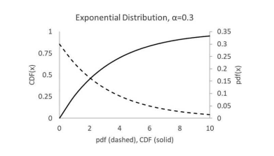
Figure $3.8$ illustrates the exponential distribution for $\alpha=0.3$. The mean and variance of the exponential distribution are
$$
\mu=\frac{1}{\alpha}
$$
and
$$
\sigma^{2}=\frac{1}{\alpha^{2}}
$$
The continuous random variable $X$ may have any units. The units on $\mu$ will be the same. The units on both $\alpha$ and $f(x)$ are the reciprocal of those of $X . F(x)$ is dimensionless. For a physical interpretation, $\alpha$ represents the fraction of events occurring per unit of space or time. The discrete geometric distribution, in its limit as the number of events is very large and the probability of success is small, approaches the continuous exponential distribution.
Example 3.10: One billion adsorption sites are available on the surface of a solid particle. Gas molecules, randomly and uniformly “looking” for a site, find one upon which to adsorb, which “hides” that site from other molecules. With an infinite gas volume, the rate at which the sites are occupied is therefore proportional to the number of unoccupied sites. If $40 \%$ of the sites are covered within the first 24 hours, how long will it take for $99 \%$ of the adsorption to be complete? What is the average lifetime of an unoccupied site?
From Equation (3.43),
$$
40 \%=0.40=F(t)=1-e^{-a t}=1-e^{-a(24)}
$$
which gives $\alpha=0.02128440 \ldots$ per hour. From Equation (3.43), $99 \%=0.99=F(t)=1-$ $e^{0.02128 .1}$, which gives $t=216.3636244$… hours or about 9 days. From Equation (3.44), $\mu=$ $1 / \alpha=46.9827645$ hours or almost 2 days.
统计代写|工程统计作业代写Engineering Statistics代考|Gamma Distribution
The gamma distribution can represent two mechanisms. In a general situation in which a number of partial random events must occur before a complete event is realized, the probability density function of the complete event is given by the gamma distribution. For instance, rust spots on your car (the partial event), may occur randomly at an average rate of one per month. If 16 spots occur before you decide to have your car repainted (the total event), the gamma distribution is the appropriate one to use to describe the repainting time interval. The gamma distribution is
$$
p d f(x)=\frac{\lambda}{\Gamma(\alpha)}(\lambda x)^{\alpha-1} \exp (-\lambda x), x \geq 0
$$
and where $\alpha$ and $\lambda>0$ and $\Gamma(\alpha)$ is the gamma function
$$
\Gamma(\alpha)=\int_{0}^{\infty} Z^{\alpha-1} e^{-z} d Z
$$
The gamma function has several properties
$$
\Gamma(\alpha)=(\alpha-1) \Gamma(\alpha-1)
$$
and if $\alpha$ is an integer, then
$$
\Gamma(\alpha)=(\alpha-1) !
$$
The variable $\alpha$ represents the number of partial events required to constitute a complete event, and $\lambda$ is the number of partial events per unit of $x$ (which may be time, distance, space, or item).
If $\alpha=1$, the gamma distribution reduces to the exponential distribution. For that reason, if an event rate is proportional to some power of $x$, then the gamma distribution can also be used as an adjusted exponential distribution. Let’s look at Example $3.10$ again. If adsorption reduces the number of gas molecules available for subsequent adsorption, then the probability of any site being occupied decreases with time. If the frequency with which gas molecules impinge on the particle surface decreases as $(\lambda x)^{a-1}$, then the gamma function describes $f(x)$. However, although close enough for most engineering applications, the power law decrease probably does not describe a real driving force exactly. For such a situation, use of the gamma distribution must be acknowledged as a convenient approximation.
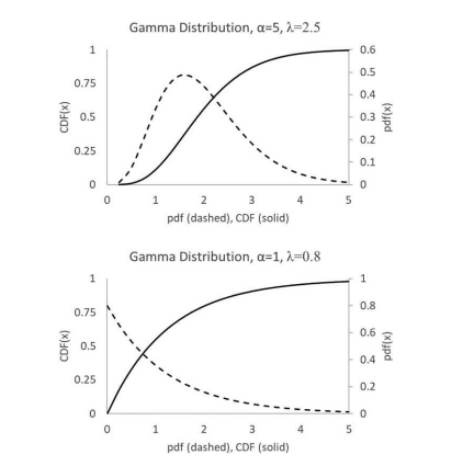
Depending on the values of $\alpha$ and $\lambda, f(x)$ may have various shapes, some of which are illustrated in Figure 3.9. A general analytical expression for $F(x)$ is intractable. For most $\alpha$ values, to obtain the cumulative distribution function, $f(x)$ must be integrated numerically. Excel provides the function GAMMA.DIST $(x, \alpha, 1 / \lambda, 0)$ to return the $p d f(x)$ value
and GAMMA.DIST $(x, \alpha, 1 / \lambda, 1)$ to return the CDF $(x)$ value. Note that the Excel parameter beta is the reciprocal of $\lambda$, here.
The mean and variance of the gamma distribution are
$$
\begin{aligned}
\mu &=\frac{\alpha}{\lambda} \
\sigma^{2} &=\frac{\alpha}{\lambda^{2}}
\end{aligned}
$$
The units of $X$ are usually count per some interval (time, distance, area, space, or item). Consequently, the units for $\lambda$ are the fraction of total failures per unit of $X$. The coefficient, $\boldsymbol{\alpha}$, is a counting number and is dimensionless, and $f(x)$ has units that are the reciprocal of the units of $X$.
统计代写|工程统计作业代写Engineering Statistics代考|Normal Distribution
The normal distribution, often called the Gaussian distribution or bell-shaped error curve, is the most widely used of all continuous probability density functions. The assumption behind this distribution is that any errors (sources of deviation from true) in the experimental results are due to the addition of many independent small perturbation sources. All experimental situations are subject to many random errors and usually yield data that can be adequately described by the normal distribution.
Even if your data is not normally distributed, the averages of data from a nonnormal distribution tend toward being normal. An average of independent samples will have some values above the mean and some below. The average will be close to the mean, and each sample would represent a small independent deviation. In the limit of large sample size, $n$, the standard deviation of the average is related to that of the individual data by $\sigma_{\bar{X}}=\sigma_{X} / \sqrt{n}$. So, when using averages, the normal distribution usually is applicable.
However, this situation is not always true. If you have any doubt that your data are distributed normally, you should use the nonparametric techniques in Chapter 7 to evaluate the distribution. Use of statistics that depend on the normal distribution for a dataset that is distinctly skewed may lead to erroneous results.
An acronym for data that is normally and independently distributed with a mean of $\mu$ and standard deviation of $\sigma$ is $\operatorname{NID}(\mu, \sigma)$.
Regardless of the shape of the distribution of the original population, the central limit theorem allows us to use the normal distribution for descriptive purposes, subject to a single restriction. The theorem simply states that if the population has a mean $\mu$ and a finite variance $\sigma^{2}$, then the distribution of the sample mean $\bar{X}$ approaches the normal distribution with mean $\mu$ and variance $\sigma^{2} / n$ as the sample size $n$ increases. The chief problem with the theorem is how to tell when the sample size is large enough to give reasonable compliance with the theorem. The selection of sample sizes is covered in Chapters 10,11 , and $17 .$
The probability density function $f(x)$ for the normal distribution is
$$
f(x)=\frac{1}{\sigma \sqrt{2 \pi}} \mathrm{e}^{\left[-\frac{1}{2}\left(\frac{x-\mu}{\sigma}\right)^{2}\right]},-\infty<x<\infty
$$
Note that the argument of the exponentiation, $\left[-\frac{1}{2}\left(\frac{x-\mu}{\sigma}\right)^{2}\right]$, must be dimensionless. As expected, $x, \mu$, and $\sigma$ each have identical units. The exponentiation value is also dimensionless. Also, since $f(x)$ is proportional to $1 / \sigma$, it has the reciprocal units of $x$.
As seen in Equation (3.52), the normal distribution has two parameters, $\mu$ and $\sigma$, which are the mean and standard deviation, respectively. The cumulative distribution function $(C D F)$, described by
$$
\operatorname{CDF}(x)=F(x)=P(X \leq x)=\frac{1}{\sigma \sqrt{2 \pi}} \int_{-\infty}^{x} e^{-(X-\mu)^{2} / 2 \sigma^{2}} d X
$$
In Equation (3.53) the variable $X$ is the generic variable, and the lower-case $x$ represents a particular value.
The logistic model, $\operatorname{CDF}(x)=F(x)=P(X \leq x)=\frac{1}{1+e^{-s(x-c)}}$, is a convenient and reasonably good approximation to the normal $C D F(x)$. Convenient: It is computationally simple, analytically invertible, and analytically differentiable. Reasonably good: Values are no more different from the normal CDF $(x)$ than that caused by uncertainty on $\mu$ and $\sigma$. For the scale factor, use $s=\sigma / 1.7$, and for the center, use $c=\mu$ (see Exercise 3.15).
工程统计代写
统计代写|工程统计作业代写Engineering Statistics代考|Continuous Distributions
指数(或负指数)分布描述了一种机制,其中在时间或距离间隔内发生故障(或事件)的概率直接取决于剩余的未失败项目的数量。它描述了诸如放射性同位素衰变、通过均匀特性物质的光强度衰减、灯泡的故障率以及颗粒在连续流动搅拌罐中的停留时间或年龄分布等事件。分布的要求是,在任何时候,任何一个特定项目失败的概率与任何其他项目失败的概率相同,并且与之前相同。另一个限制是数字太大以至于测量值似乎是连续的。概率分布函数是
pdF(X)=一种和−一种X,0≤X≤∞,一种>0
和
F(X)=1−和−一种X
变量X表示时间或距离间隔,而不是未失败项目的数量(或其他一些数量度量)。指数的参数必须是无量纲的,
所以单位一种是单位的倒数X. 这需要在单位pdF(X)也是单位的倒数X, 制造pdF(X)成为一个比率。
数字3.8说明了指数分布一种=0.3. 指数分布的均值和方差为
μ=1一种
和
σ2=1一种2
连续随机变量X可以有任何单位。上的单位μ将是相同的。双方的单位一种和F(X)是那些的倒数X.F(X)是无量纲的。对于物理解释,一种表示每单位空间或时间发生的事件的比例。离散几何分布,由于事件数量很大,成功概率很小,接近连续指数分布。
示例 3.10:固体颗粒表面有十亿个吸附位点。气体分子随机且均匀地“寻找”一个位点,找到一个要吸附的位点,从而使该位点对其他分子“隐藏”。因此,在无限气体体积的情况下,站点被占用的速率与未占用站点的数量成正比。如果40%的网站在前 24 小时内覆盖,需要多长时间99%吸附完成?空置站点的平均寿命是多少?
从方程(3.43),
40%=0.40=F(吨)=1−和−一种吨=1−和−一种(24)
这使一种=0.02128440…每小时。从方程(3.43),99%=0.99=F(吨)=1− 和0.02128.1, 这使吨=216.3636244… 小时或大约 9 天。从方程(3.44),μ= 1/一种=46.9827645小时或将近 2 天。
统计代写|工程统计作业代写Engineering Statistics代考|Gamma Distribution
伽马分布可以代表两种机制。在实现一个完整事件之前必须发生许多部分随机事件的一般情况下,完整事件的概率密度函数由伽马分布给出。例如,您的汽车上的锈斑(部分事件)可能以平均每月一个的速度随机出现。如果在您决定重新粉刷汽车(整个事件)之前出现 16 个点,则伽马分布是用于描述重新粉刷时间间隔的合适分布。伽马分布是
pdF(X)=λΓ(一种)(λX)一种−1经验(−λX),X≥0
和在哪里一种和λ>0和Γ(一种)是伽马函数
Γ(一种)=∫0∞从一种−1和−和d从
伽马函数有几个属性
Γ(一种)=(一种−1)Γ(一种−1)
而如果一种是一个整数,那么
Γ(一种)=(一种−1)!
变量一种表示构成完整事件所需的部分事件的数量,并且λ是每单位的部分事件数X(可能是时间、距离、空间或项目)。
如果一种=1,伽马分布减少到指数分布。因此,如果事件发生率与X,则伽马分布也可以用作调整后的指数分布。我们来看例子3.10再次。如果吸附减少了可用于后续吸附的气体分子的数量,那么任何位点被占据的概率都会随着时间的推移而降低。如果气体分子撞击颗粒表面的频率降低为(λX)一种−1,则伽马函数描述F(X). 然而,尽管对于大多数工程应用来说已经足够接近,但幂律下降可能并不能准确地描述真正的驱动力。对于这种情况,必须承认使用伽马分布是一种方便的近似。
取决于的值一种和λ,F(X)可能有各种形状,其中一些如图 3.9 所示。的一般解析表达式F(X)是棘手的。对于大多数一种值,以获得累积分布函数,F(X)必须进行数值积分。Excel 提供函数 GAMMA.DIST(X,一种,1/λ,0)返回pdF(X)价值
和 GAMMA.DIST(X,一种,1/λ,1)归还 CDF(X)价值。请注意,Excel 参数 beta 是λ, 这里。
伽马分布的均值和方差为
μ=一种λ σ2=一种λ2
的单位X通常按某个间隔(时间、距离、面积、空间或项目)计算。因此,单位为λ是每单位总故障的比例X. 系数,一种, 是一个计数并且是无量纲的,并且F(X)有单位是单位的倒数X.
统计代写|工程统计作业代写Engineering Statistics代考|Normal Distribution
正态分布,通常称为高斯分布或钟形误差曲线,是所有连续概率密度函数中使用最广泛的。这种分布背后的假设是,实验结果中的任何误差(偏离真实的来源)都是由于添加了许多独立的小扰动源。所有实验情况都会受到许多随机误差的影响,并且通常会产生可以用正态分布充分描述的数据。
即使您的数据不是正态分布的,来自非正态分布的数据的平均值也趋于正态分布。独立样本的平均值将具有一些高于平均值和一些低于平均值的值。平均值将接近平均值,并且每个样本将代表一个小的独立偏差。在大样本量的限制下,n, 平均值的标准差与单个数据的标准差相关σX¯=σX/n. 因此,在使用平均值时,通常适用正态分布。
然而,这种情况并非总是如此。如果你对你的数据是否正态分布有任何疑问,你应该使用第 7 章中的非参数技术来评估分布。对于明显偏斜的数据集,使用依赖于正态分布的统计数据可能会导致错误的结果。
正态且独立分布的数据的首字母缩写词,均值为μ和标准差σ是不是(μ,σ).
不管原始种群分布的形状如何,中心极限定理允许我们使用正态分布进行描述,但要受到单一限制。该定理简单地说,如果总体有一个均值μ和有限方差σ2, 那么样本均值的分布X¯均值接近正态分布μ和方差σ2/n作为样本量n增加。该定理的主要问题是如何判断样本量何时足够大以合理地符合该定理。第 10,11 章介绍了样本量的选择,以及17.
概率密度函数F(X)因为正态分布是
F(X)=1σ2圆周率和[−12(X−μσ)2],−∞<X<∞
请注意,取幂的参数,[−12(X−μσ)2], 必须是无量纲的。正如预期的那样,X,μ, 和σ每个都有相同的单位。取幂值也是无量纲的。另外,由于F(X)正比于1/σ, 它的倒数单位为X.
如公式 (3.52) 所示,正态分布有两个参数,μ和σ,分别是平均值和标准差。累积分布函数(CDF),描述为
CDF(X)=F(X)=磷(X≤X)=1σ2圆周率∫−∞X和−(X−μ)2/2σ2dX
在方程 (3.53) 中,变量X是泛型变量,小写X代表一个特定的值。
逻辑模型,CDF(X)=F(X)=磷(X≤X)=11+和−s(X−C), 是一个方便且相当好的近似法线CDF(X). 方便:计算简单,解析可逆,解析可微。相当不错:值与正常的 CDF 没有什么不同(X)比由不确定性引起的μ和σ. 对于比例因子,使用s=σ/1.7,对于中心,使用C=μ(见习题 3.15)。

统计代写请认准statistics-lab™. statistics-lab™为您的留学生涯保驾护航。
金融工程代写
金融工程是使用数学技术来解决金融问题。金融工程使用计算机科学、统计学、经济学和应用数学领域的工具和知识来解决当前的金融问题,以及设计新的和创新的金融产品。
非参数统计代写
非参数统计指的是一种统计方法,其中不假设数据来自于由少数参数决定的规定模型;这种模型的例子包括正态分布模型和线性回归模型。
广义线性模型代考
广义线性模型(GLM)归属统计学领域,是一种应用灵活的线性回归模型。该模型允许因变量的偏差分布有除了正态分布之外的其它分布。
术语 广义线性模型(GLM)通常是指给定连续和/或分类预测因素的连续响应变量的常规线性回归模型。它包括多元线性回归,以及方差分析和方差分析(仅含固定效应)。
有限元方法代写
有限元方法(FEM)是一种流行的方法,用于数值解决工程和数学建模中出现的微分方程。典型的问题领域包括结构分析、传热、流体流动、质量运输和电磁势等传统领域。
有限元是一种通用的数值方法,用于解决两个或三个空间变量的偏微分方程(即一些边界值问题)。为了解决一个问题,有限元将一个大系统细分为更小、更简单的部分,称为有限元。这是通过在空间维度上的特定空间离散化来实现的,它是通过构建对象的网格来实现的:用于求解的数值域,它有有限数量的点。边界值问题的有限元方法表述最终导致一个代数方程组。该方法在域上对未知函数进行逼近。[1] 然后将模拟这些有限元的简单方程组合成一个更大的方程系统,以模拟整个问题。然后,有限元通过变化微积分使相关的误差函数最小化来逼近一个解决方案。
tatistics-lab作为专业的留学生服务机构,多年来已为美国、英国、加拿大、澳洲等留学热门地的学生提供专业的学术服务,包括但不限于Essay代写,Assignment代写,Dissertation代写,Report代写,小组作业代写,Proposal代写,Paper代写,Presentation代写,计算机作业代写,论文修改和润色,网课代做,exam代考等等。写作范围涵盖高中,本科,研究生等海外留学全阶段,辐射金融,经济学,会计学,审计学,管理学等全球99%专业科目。写作团队既有专业英语母语作者,也有海外名校硕博留学生,每位写作老师都拥有过硬的语言能力,专业的学科背景和学术写作经验。我们承诺100%原创,100%专业,100%准时,100%满意。
随机分析代写
随机微积分是数学的一个分支,对随机过程进行操作。它允许为随机过程的积分定义一个关于随机过程的一致的积分理论。这个领域是由日本数学家伊藤清在第二次世界大战期间创建并开始的。
时间序列分析代写
随机过程,是依赖于参数的一组随机变量的全体,参数通常是时间。 随机变量是随机现象的数量表现,其时间序列是一组按照时间发生先后顺序进行排列的数据点序列。通常一组时间序列的时间间隔为一恒定值(如1秒,5分钟,12小时,7天,1年),因此时间序列可以作为离散时间数据进行分析处理。研究时间序列数据的意义在于现实中,往往需要研究某个事物其随时间发展变化的规律。这就需要通过研究该事物过去发展的历史记录,以得到其自身发展的规律。
回归分析代写
多元回归分析渐进(Multiple Regression Analysis Asymptotics)属于计量经济学领域,主要是一种数学上的统计分析方法,可以分析复杂情况下各影响因素的数学关系,在自然科学、社会和经济学等多个领域内应用广泛。
MATLAB代写
MATLAB 是一种用于技术计算的高性能语言。它将计算、可视化和编程集成在一个易于使用的环境中,其中问题和解决方案以熟悉的数学符号表示。典型用途包括:数学和计算算法开发建模、仿真和原型制作数据分析、探索和可视化科学和工程图形应用程序开发,包括图形用户界面构建MATLAB 是一个交互式系统,其基本数据元素是一个不需要维度的数组。这使您可以解决许多技术计算问题,尤其是那些具有矩阵和向量公式的问题,而只需用 C 或 Fortran 等标量非交互式语言编写程序所需的时间的一小部分。MATLAB 名称代表矩阵实验室。MATLAB 最初的编写目的是提供对由 LINPACK 和 EISPACK 项目开发的矩阵软件的轻松访问,这两个项目共同代表了矩阵计算软件的最新技术。MATLAB 经过多年的发展,得到了许多用户的投入。在大学环境中,它是数学、工程和科学入门和高级课程的标准教学工具。在工业领域,MATLAB 是高效研究、开发和分析的首选工具。MATLAB 具有一系列称为工具箱的特定于应用程序的解决方案。对于大多数 MATLAB 用户来说非常重要,工具箱允许您学习和应用专业技术。工具箱是 MATLAB 函数(M 文件)的综合集合,可扩展 MATLAB 环境以解决特定类别的问题。可用工具箱的领域包括信号处理、控制系统、神经网络、模糊逻辑、小波、仿真等。