如果你也在 怎样代写时间序列分析这个学科遇到相关的难题,请随时右上角联系我们的24/7代写客服。
时间序列分析是分析在一个时间间隔内收集的一系列数据点的具体方式。在时间序列分析中,分析人员在设定的时间段内以一致的时间间隔记录数据点,而不仅仅是间歇性或随机地记录数据点。
statistics-lab™ 为您的留学生涯保驾护航 在代写时间序列分析方面已经树立了自己的口碑, 保证靠谱, 高质且原创的统计Statistics代写服务。我们的专家在代写时间序列分析代写方面经验极为丰富,各种代写时间序列分析相关的作业也就用不着说。
我们提供的时间序列分析及其相关学科的代写,服务范围广, 其中包括但不限于:
- Statistical Inference 统计推断
- Statistical Computing 统计计算
- Advanced Probability Theory 高等概率论
- Advanced Mathematical Statistics 高等数理统计学
- (Generalized) Linear Models 广义线性模型
- Statistical Machine Learning 统计机器学习
- Longitudinal Data Analysis 纵向数据分析
- Foundations of Data Science 数据科学基础
统计代写|时间序列分析作业代写time series analysis代考|Determining the Order of Autoregressive Models
Seemingly, the availability of an exact formula for the spectral density means that the frequency resolution of autoregressive and other parametric spectral estimates is infinitely high because it can be calculated at any frequency. However, as follows from Eq. (3.13), the number of peaks, troughs, and inflection points in autoregressive spectral density estimates cannot exceed the model’s order $p$. Therefore, the AR order is the key parameter that defines the features of an AR (or MEM) spectral estimate. Similar considerations are true for the moving average and mixed ARMA models.
The role of the order $p$ is convenient to characterize with the following simple example. Let $x_{t}, t=1, \ldots 100$, be a sample record of a dimensionless white noise process with a unit variance and the sampling interval $\Delta t$ (e.g., 1 year, 1 day, etc.). According to Eq. (3.13), the true spectrum is a constant: $s(f)=2 \sigma_{a}^{2} \Delta t$. As the true model of the time series is not known at the initial stage of analysis, the spectral estimates should be sought for several values of $p$, say, from $p=0$ through $p=10$ for a time series of length $N=100$. To select higher values of the AR order would be unreasonable because of common sense considerations: it is not possible to obtain reliable estimates if the number of quantities to be estimated is comparable to the number of observations. The results of analysis of the white noise sequence are shown in Fig. 3.1. Obviously, if one were to choose the AR order $p=10$ arbitrarily, the conclusion would be that the time series contains “cycles” or quasi-periodic components at frequencies about $0.11$ cycles per $\Delta t(\mathrm{cp} \Delta t)$ and $0.39 \mathrm{cp} \Delta t$. However, the correctly defined confidence limits for the estimates given in Fig. $3.1$ show that such conclusions would have been false because one can draw a very smooth or even a horizontal line within the confidence interval for the estimate. Obviously, a high order (e.g., $p \geq 10$ ) does not necessarily mean that the spectral density contains significant peaks. An AR model having a high order may have a very smooth spectrum, while a low-order model can have very sharp peaks (see Fig. $2.8$ and the well-known AR(4) example given in the Percival and Walden book published in 1993, pp. 46, 148). Similar examples can be given for more complicated spectra, but the major conclusion is that determining the order of parametric models and showing a confidence interval constitute the absolutely necessary element of parametric spectral analysis.
Several methods can be used to determine the optimal order of an autoregressive model that is being fitted to a time series, but the best approach is to use the order selection criteria (OSC) developed in information theory. Such criteria recommend an optimal order by finding a compromise solution for the following dilemma: a higher order may reveal more details in the spectral density estimate, but at the same time a higher order means that the estimates of AR coefficients are less reliable. The order recommended by order selection criteria is optimal in the sense that it minimizes the variance of innovation sequence-the absolutely unpredictable component of the time series and takes into account the loss of reliability of estimates with the growing AR order. Several such OSCs are known and considered reliable for determining the AR order.
统计代写|时间序列分析作业代写time series analysis代考|Comparison of Autoregressive and Nonparametric
The statement that the spectral density is the most important statistics of any scalar time series is true for Gaussian and non-Gaussian data. The spectral density can be estimated with parametric and nonparametric methods, and if the time series is long, the estimates will be reliable and similar to each other. If the time series is short, which happens regularly in climatology and its branches and in other Earth sciences, the task of proper spectral analysis becomes vital. In this section, we will show the advantages of the parametric approach to the task of spectral estimation, which exist, in particular, due to the fact that many geophysical processes can be well approximated with stochastic difference equations of relatively low order. The examples given here include time series whose spectra are typical for climatic processes, including the
annual global surface temperature. The time series will always be short: the total number of its terms is just 50 . The autoregressive spectral estimates will be compared with respective nonparametric estimates obtained according to Blackman and Tukey (1958). Four time series of length $N=50$ have AR orders from 1 to 4 , and they are quite common for climate and for other geophysical phenomena. The true AR models are known in all cases, and the initial data for the analysis were obtained through simulation. Because of the small length of the time series, the sample estimates of AR coefficients may differ rather significantly from the true values.
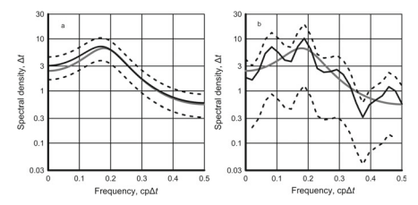
The true model of the first time series is an $\operatorname{AR}(1)$ with the AR coefficient $\varphi=0.5$. It can be the annual river streamflow, daily temperature, sea level variations in coastal areas with no tides, etc. The sample AR (or MEM) estimate of the spectrum is shown in Fig. 3.3a along with the true spectrum.
According to Fig. $3.3 \mathrm{a}$, the $90 \%$ confidence interval for the AR spectral estimate contains the true spectrum; this estimate can be regarded as satisfactory. The shape of the spectrum is reproduced accurately, and the bias occurs due to the sampling variability of the variance estimate. The nonparametric estimate (Fig. 3.3b) has several peaks, but the peaks are statistically insignificant. The $90 \%$ confidence interval is wide and asymmetric with respect to the spectral estimate due to the asymmetry of $\chi^{2}$ distribution at low degrees of freedom in this and the other three examples below.
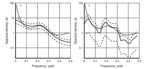
More complicated AR models are shown in Figs. 3.4, 3.5, and 3.6. In the first case, the true model is $\operatorname{AR}(2)$ with AR coefficients $\varphi_{1}=0.5$ and $\varphi_{2}=-0.4$. The true spectrum is close to the spectrum of the Southern Oscillation Index. The characteristic equation of this model is
cases, the natural frequency of the system is approximately $0.23 \Delta t^{-1}$. The estimate for the AR(3) time series, which simulates the Palmer Draught Severity Index over the contiguous USA, stays close to the true spectral density for the AR(3) time series (Fig. 3.5a) and becomes less accurate for the $\mathrm{AR}(4)$ time series (Fig. 3.6a). However, the shape of the spectrum is reproduced rather accurately including the hump at intermediate frequencies. This simulated time series is similar to the actual annual global surface temperature (Privalsky and Yushkov 2018). In all cases, the nonparametric estimates given in Figs. $3.5 \mathrm{~b}$ and $3.6 \mathrm{~b}$ are less accurate, but one has to remember that the time series are very short for the nonparametric spectral estimation to be efficient. The incorrect behavior of the spectral estimates at low frequencies in Fig. $3.6$ is the results of a poor estimate of the time series variance due to its short length.
These examples are given here to illustrate the following argument: when the optimal autoregressive model of a geophysical or any other time series indicated by order selection criteria is low, the autoregressive approach allows one to obtain statistically reliable estimates of AR coefficients and, consequently, of the spectral density even when the time series is very short. Also, a low AR order does not necessarily mean that the spectrum of the time series does not contain any sharp peaks.
统计代写|时间序列分析作业代写time series analysis代考|Advantages and Disadvantages of Autoregressive
The autoregressive approach provides quantitative information about statistical properties of time series in both time and frequency domains. This can also be achieved with other parametric models, but the moving average operator is less reasonable physically and is difficult to deal with. The nonparametric methods of analysis do not produce explicit information about the time series behavior in the time domain and, if the time series is short, the nonparametric spectral estimates are less reliable than the AR estimates.
The autoregressive stochastic difference equation possesses a number of useful features for analysis of stationary time series:
- it presents a ready-to-use tool for linear extrapolation of time series (Chap. 6);
- it allows one to get quantitative estimates of time series dependence upon its previous values (up to the AR order $p$ ) and upon the innovation sequence;
- it can be used to determine the natural frequencies and damping coefficients of the time series, that is, the frequencies, at which the spectral density may have peaks;
- it provides an analytical expression for the time series spectral density;
- the autoregressive approach to spectral estimation satisfies the requirements of the maximum entropy method (MEM), and it is capable of producing satisfactory estimates of the spectrum when the time series is short.
This author is not aware of any disadvantages in applying the autoregressive time and frequency domain approach to time series research in climatology and other Earth and solar sciences.
时间序列分析代写
统计代写|时间序列分析作业代写time series analysis代考|Determining the Order of Autoregressive Models
看起来,谱密度的精确公式的可用性意味着自回归和其他参数谱估计的频率分辨率是无限高的,因为它可以在任何频率下计算。但是,如下式所示。(3.13),自回归谱密度估计中的波峰、波谷和拐点的数量不能超过模型的阶数p. 因此,AR 阶是定义 AR(或 MEM)谱估计特征的关键参数。移动平均和混合 ARMA 模型也有类似的考虑。
命令的作用p用下面的简单例子来表征很方便。让X吨,吨=1,…100,是具有单位方差和采样间隔的无量纲白噪声过程的样本记录Δ吨(例如,1 年、1 天等)。根据方程式。(3.13),真谱是一个常数:s(F)=2σ一种2Δ吨. 由于时间序列的真实模型在分析的初始阶段是未知的,因此应该为几个值寻找谱估计p,比如说,从p=0通过p=10对于长度的时间序列ñ=100. 出于常识考虑,选择更高的 AR 阶值是不合理的:如果要估计的数量的数量与观察的数量相当,则不可能获得可靠的估计。白噪声序列的分析结果如图 3.1 所示。显然,如果要选择 AR 订单p=10任意地,结论将是时间序列包含“周期”或准周期分量,频率约为0.11每周期Δ吨(CpΔ吨)和0.39CpΔ吨. 然而,图 2 中给出的估计值的正确定义的置信限。3.1表明这样的结论是错误的,因为人们可以在估计的置信区间内绘制一条非常平滑甚至水平的线。显然,高阶(例如,p≥10) 并不一定意味着光谱密度包含显着的峰值。具有高阶的 AR 模型可能具有非常平滑的光谱,而低阶模型可能具有非常尖锐的峰(见图 1)。2.8以及在 1993 年出版的 Percival 和 Walden 书中给出的著名 AR(4) 示例,第 46、148 页)。对于更复杂的光谱可以给出类似的例子,但主要结论是确定参数模型的顺序和显示置信区间构成了参数光谱分析的绝对必要元素。
有几种方法可用于确定适合时间序列的自回归模型的最佳顺序,但最好的方法是使用信息论中开发的顺序选择标准 (OSC)。这些标准通过为以下困境找到折衷解决方案来推荐最佳阶数:更高阶可能会在谱密度估计中揭示更多细节,但同时更高阶意味着 AR 系数的估计不太可靠。订单选择标准推荐的订单是最优的,因为它最小化了创新序列的方差 – 时间序列的绝对不可预测的组件,并考虑了随着 AR 订单的增长而失去估计的可靠性。几个这样的 OSC 是已知的并且被认为对于确定 AR 顺序是可靠的。
统计代写|时间序列分析作业代写time series analysis代考|Comparison of Autoregressive and Nonparametric
对于高斯和非高斯数据,谱密度是任何标量时间序列中最重要的统计量这一说法是正确的。谱密度可以用参数和非参数方法估计,如果时间序列很长,估计将是可靠的并且彼此相似。如果时间序列很短,这在气候学及其分支和其他地球科学中经常发生,那么适当的光谱分析任务就变得至关重要。在本节中,我们将展示参数方法在光谱估计任务中的优势,特别是由于许多地球物理过程可以用相对低阶的随机差分方程很好地近似这一事实而存在。这里给出的例子包括时间序列,其光谱是典型的气候过程,包括
年全球地表温度。时间序列总是很短:它的项总数只有 50 。自回归谱估计将与根据 Blackman 和 Tukey (1958) 获得的相应非参数估计进行比较。四个时间序列的长度ñ=50AR 阶数从 1 到 4 ,它们在气候和其他地球物理现象中很常见。真正的 AR 模型在所有情况下都是已知的,用于分析的初始数据是通过模拟获得的。由于时间序列的长度较小,AR 系数的样本估计值可能与真实值有很大差异。
第一个时间序列的真实模型是和(1)与 AR 系数披=0.5. 它可以是年河流流量、日温度、沿海地区无潮汐的海平面变化等。光谱的样本 AR(或 MEM)估计与真实光谱一起显示在图 3.3a 中。
根据图。3.3一种, 这90%AR 谱估计的置信区间包含真实谱;这个估计可以认为是令人满意的。谱的形状被准确地再现,并且由于方差估计的抽样变异性而出现偏差。非参数估计(图 3.3b)有几个峰值,但峰值在统计上不显着。这90%由于频谱估计的不对称性,置信区间很宽且不对称χ2在这个和下面的其他三个例子中,分布在低自由度。
更复杂的 AR 模型如图 1 所示。3.4、3.5 和 3.6。在第一种情况下,真实模型是和(2)具有 AR 系数披1=0.5和披2=−0.4. 真实光谱接近南方涛动指数的光谱。该模型的特征方程为
情况下,系统的固有频率约为0.23Δ吨−1. AR(3) 时间序列的估计值模拟了美国邻近地区的 Palmer Draft Severity Index,它与 AR(3) 时间序列的真实光谱密度保持接近(图 3.5a),并且对于一种R(4)时间序列(图 3.6a)。然而,频谱的形状被相当准确地再现,包括中频的驼峰。这个模拟的时间序列类似于实际的年度全球地表温度(Privalsky 和 Yushkov 2018)。在所有情况下,图 2 中给出的非参数估计。3.5 b和3.6 b不太准确,但必须记住时间序列非常短,非参数谱估计是有效的。图 3 中低频频谱估计的不正确行为。3.6是由于长度短而对时间序列方差的估计不佳的结果。
在这里给出这些例子来说明以下论点:当地球物理或任何其他由顺序选择标准指示的时间序列的最佳自回归模型较低时,自回归方法允许人们获得统计上可靠的 AR 系数估计值,因此,即使时间序列很短,谱密度也是如此。此外,低 AR 阶并不一定意味着时间序列的频谱不包含任何尖峰。
统计代写|时间序列分析作业代写time series analysis代考|Advantages and Disadvantages of Autoregressive
自回归方法提供有关时间序列在时域和频域中的统计特性的定量信息。这也可以通过其他参数模型来实现,但移动平均算子在物理上不太合理,难以处理。非参数分析方法不会产生有关时域中时间序列行为的明确信息,如果时间序列很短,则非参数谱估计不如 AR 估计可靠。
自回归随机差分方程具有许多用于分析平稳时间序列的有用特征:
- 它为时间序列的线性外推提供了一个现成的工具(第 6 章);
- 它允许人们根据其先前的值(直到 AR 顺序)获得时间序列依赖的定量估计p) 和创新序列;
- 它可用于确定时间序列的固有频率和阻尼系数,即频谱密度可能出现峰值的频率;
- 它提供了时间序列谱密度的解析表达式;
- 谱估计的自回归方法满足最大熵法(MEM)的要求,并且能够在时间序列较短的情况下产生令人满意的谱估计。
作者没有意识到将自回归时域和频域方法应用于气候学和其他地球和太阳科学的时间序列研究的任何缺点。

统计代写请认准statistics-lab™. statistics-lab™为您的留学生涯保驾护航。
金融工程代写
金融工程是使用数学技术来解决金融问题。金融工程使用计算机科学、统计学、经济学和应用数学领域的工具和知识来解决当前的金融问题,以及设计新的和创新的金融产品。
非参数统计代写
非参数统计指的是一种统计方法,其中不假设数据来自于由少数参数决定的规定模型;这种模型的例子包括正态分布模型和线性回归模型。
广义线性模型代考
广义线性模型(GLM)归属统计学领域,是一种应用灵活的线性回归模型。该模型允许因变量的偏差分布有除了正态分布之外的其它分布。
术语 广义线性模型(GLM)通常是指给定连续和/或分类预测因素的连续响应变量的常规线性回归模型。它包括多元线性回归,以及方差分析和方差分析(仅含固定效应)。
有限元方法代写
有限元方法(FEM)是一种流行的方法,用于数值解决工程和数学建模中出现的微分方程。典型的问题领域包括结构分析、传热、流体流动、质量运输和电磁势等传统领域。
有限元是一种通用的数值方法,用于解决两个或三个空间变量的偏微分方程(即一些边界值问题)。为了解决一个问题,有限元将一个大系统细分为更小、更简单的部分,称为有限元。这是通过在空间维度上的特定空间离散化来实现的,它是通过构建对象的网格来实现的:用于求解的数值域,它有有限数量的点。边界值问题的有限元方法表述最终导致一个代数方程组。该方法在域上对未知函数进行逼近。[1] 然后将模拟这些有限元的简单方程组合成一个更大的方程系统,以模拟整个问题。然后,有限元通过变化微积分使相关的误差函数最小化来逼近一个解决方案。
tatistics-lab作为专业的留学生服务机构,多年来已为美国、英国、加拿大、澳洲等留学热门地的学生提供专业的学术服务,包括但不限于Essay代写,Assignment代写,Dissertation代写,Report代写,小组作业代写,Proposal代写,Paper代写,Presentation代写,计算机作业代写,论文修改和润色,网课代做,exam代考等等。写作范围涵盖高中,本科,研究生等海外留学全阶段,辐射金融,经济学,会计学,审计学,管理学等全球99%专业科目。写作团队既有专业英语母语作者,也有海外名校硕博留学生,每位写作老师都拥有过硬的语言能力,专业的学科背景和学术写作经验。我们承诺100%原创,100%专业,100%准时,100%满意。
随机分析代写
随机微积分是数学的一个分支,对随机过程进行操作。它允许为随机过程的积分定义一个关于随机过程的一致的积分理论。这个领域是由日本数学家伊藤清在第二次世界大战期间创建并开始的。
时间序列分析代写
随机过程,是依赖于参数的一组随机变量的全体,参数通常是时间。 随机变量是随机现象的数量表现,其时间序列是一组按照时间发生先后顺序进行排列的数据点序列。通常一组时间序列的时间间隔为一恒定值(如1秒,5分钟,12小时,7天,1年),因此时间序列可以作为离散时间数据进行分析处理。研究时间序列数据的意义在于现实中,往往需要研究某个事物其随时间发展变化的规律。这就需要通过研究该事物过去发展的历史记录,以得到其自身发展的规律。
回归分析代写
多元回归分析渐进(Multiple Regression Analysis Asymptotics)属于计量经济学领域,主要是一种数学上的统计分析方法,可以分析复杂情况下各影响因素的数学关系,在自然科学、社会和经济学等多个领域内应用广泛。
MATLAB代写
MATLAB 是一种用于技术计算的高性能语言。它将计算、可视化和编程集成在一个易于使用的环境中,其中问题和解决方案以熟悉的数学符号表示。典型用途包括:数学和计算算法开发建模、仿真和原型制作数据分析、探索和可视化科学和工程图形应用程序开发,包括图形用户界面构建MATLAB 是一个交互式系统,其基本数据元素是一个不需要维度的数组。这使您可以解决许多技术计算问题,尤其是那些具有矩阵和向量公式的问题,而只需用 C 或 Fortran 等标量非交互式语言编写程序所需的时间的一小部分。MATLAB 名称代表矩阵实验室。MATLAB 最初的编写目的是提供对由 LINPACK 和 EISPACK 项目开发的矩阵软件的轻松访问,这两个项目共同代表了矩阵计算软件的最新技术。MATLAB 经过多年的发展,得到了许多用户的投入。在大学环境中,它是数学、工程和科学入门和高级课程的标准教学工具。在工业领域,MATLAB 是高效研究、开发和分析的首选工具。MATLAB 具有一系列称为工具箱的特定于应用程序的解决方案。对于大多数 MATLAB 用户来说非常重要,工具箱允许您学习和应用专业技术。工具箱是 MATLAB 函数(M 文件)的综合集合,可扩展 MATLAB 环境以解决特定类别的问题。可用工具箱的领域包括信号处理、控制系统、神经网络、模糊逻辑、小波、仿真等。