如果你也在 怎样代写生物统计biostatistics这个学科遇到相关的难题,请随时右上角联系我们的24/7代写客服。
生物统计学是将统计技术应用于健康相关领域的科学研究,包括医学、生物学和公共卫生,并开发新的工具来研究这些领域。
statistics-lab™ 为您的留学生涯保驾护航 在代写生物统计biostatistics方面已经树立了自己的口碑, 保证靠谱, 高质且原创的统计Statistics代写服务。我们的专家在代写生物统计biostatistics代写方面经验极为丰富,各种生物统计biostatistics相关的作业也就用不着说。
我们提供的生物统计biostatistics及其相关学科的代写,服务范围广, 其中包括但不限于:
- Statistical Inference 统计推断
- Statistical Computing 统计计算
- Advanced Probability Theory 高等概率论
- Advanced Mathematical Statistics 高等数理统计学
- (Generalized) Linear Models 广义线性模型
- Statistical Machine Learning 统计机器学习
- Longitudinal Data Analysis 纵向数据分析
- Foundations of Data Science 数据科学基础
统计代写|生物统计代写biostatistics代考|Qualitative Variables
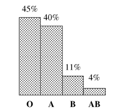
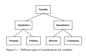
Qualitative variables take on nonnumeric values and are usually used to represent a distinct quality of a population unit. When the possible values of a qualitative variable have no intrinsic ordering, the variable is called a nominal variable; when there is a natural ordering of the possible values of the variable, then the variable is called an ordinal variable. An example of a nominal variable is Blood Type where the standard values for blood type are $\mathrm{A}, \mathrm{B}, \mathrm{AB}$, and $\mathrm{O}$. Clearly, there is no intrinsic ordering of these blood types, and hence, Blood Type is a nominal variable. An example of an ordinal variable is the variable Pain where a subject is asked to describe their pain verbally as
- No pain,
- Mild pain,
- Discomforting pain,
- Distressing pain,
- Intense pain,
- Excruciating pain.
In this case, since the verbal descriptions describe increasing levels of pain, there is a clear ordering of the possible values of the variable Pain levels, and therefore, Pain is an ordinal qualitative variable.
Example 2.2
In the Framingham Heart Study of coronary heart disease, the following two nominal qualitative variables were recorded:
$$
\text { Smokes }=\left{\begin{array}{l}
\text { Yes } \
\text { No }
\end{array}\right.
$$ - and
- $$
- \text { Diabetes }=\left{\begin{array}{l}
- \text { Yes } \
- \text { No }
- \end{array}\right.
- $$
- Example $2.3$
- An example of an ordinal variable is the variable Baldness when measured on the Norwood-Hamilton scale for male-pattern baldness. The variable Baldness is measured according to the seven categories listed below:
- I Full head of hair without any hair loss.
- II Minor recession at the front of the hairline.
- III Further loss at the front of the hairline, which is considered “cosmetically significant.”
- IV Progressively more loss along the front hairline and at the crown.
- V Hair loss extends toward the vertex.
- VI Frontal and vertex balding areas merge into one and increase in size.
- VII All hair is lost along the front hairline and crown.
- Clearly, the values of the variable Baldness indicate an increasing degree of hair loss, and thus, Baldness as measured on the Norwood-Hamilton scale is an ordinal variable. This variable is also measured on the Offspring Cohort in the Framingham Heart Study.
统计代写|生物统计代写biostatistics代考|A quantitative variable
A quantitative variable is a variable that takes only numeric values. The values of a quantitative variable are said to be measured on an interval scale when the difference between two values is meaningful; the values of a quantitative variable are said to be measured on a ratio scale when the ratio of two values is meaningful. The key difference between a variable measured on an interval scale and a ratio scale is that on a ratio scale there is a “natural zero” representing absence of the attribute being measured, while there is no natural zero for variables measured on only an interval scale. Some scales of measurement will have natural zero and some will not. When a measurement scale has a natural zero, then the ratio of two measurements is a meaningful measure of how many times larger one value is than the other. For example, the variable Fat that represents the grams of fat in a food product is measured on a ratio scale because the value Fat $=0$ indicates that the unit contained absolutely no fat. When a scale of measurement does not have a natural zero, then only the difference between two measurements is a meaningful comparison of the values of the two measurements. For example, the variable Body Temperature is measured on a scale that has no natural zero since Body Temperature $=0$ does not indicate that the body has no temperature.
Since interval scales are ordered, the difference between two values measures how much larger one value is than another. A ratio scale is also an interval scale but has the additional property that the ratio of two values is meaningful. Thus, for a variable measured on an interval scale the difference of two values is the meaningful way to compare the values, and for a variable measured on a ratio scale both the difference and the ratio of two values are meaningful ways to compare difference values of the variable. For example, body temperature in degrees Fahrenheit is a variable that is measured on an interval scale so that it is meaningful to say that a body temperature of $98.6$ and a body temperature of $102.3$ differ by $3.7$ degrees; however, it would not be meaningful to say that a temperature of $102.3$ is $1.04$ times as much as a temperature of $98.6$. On the other hand, the variable weight in pounds is measured on a ratio scale, and therefore, it would be proper to say that a weight of $210 \mathrm{lb}$ is $1.4$ times a weight of $150 \mathrm{lb}$; it would also be meaningful to say that a weight of $210 \mathrm{lb}$ is $60 \mathrm{lb}$ more than a weight of $150 \mathrm{lb}$.
统计代写|生物统计代写biostatistics代考|Multivariate Data
In most research problems, there will be many variables that need to be measured. When the collection of variables measured on each unit consists of two or more variables, a data set is called a multivariate data set, and a multivariate data set consisting of only two variables is called a bivariate data set. In a multivariate data set, there is usually one variable that is of primary interest to a research question that is believed to be explained by some of the other variables measured in the study. The variable of primary interest is called a response variable and the variables believed to cause changes in the response are called explanatory variables or predictor variables. The explanatory variables are often referred to as the input variables and the response variable is often referred to as the output variable. Furthermore, in a statistical model, the response variable is the variable that is being modeled; the explanatory variables are the input variables in the model that are believed to cause or explain differences in the response variable. For example, in studying the survival of melanoma patients, the response variable might be Survival Time that is expected to be influenced by the explanatory variables Age, Gender, Clark’s Stage, and Tumor Size. In this case, a model relating Survival Time to the explanatory variables Age, Gender, Clark’s Stage, and Tumor Size might be investigated in the research study.
A multivariate data set often consists of a mixture of qualitative and quantitative variables. For example, in a biomedical study, several variables that are commonly measured are a subject’s age, race, gender, height, and weight. When data have been collected, the multivariate data set is generally stored in a spreadsheet with the columns containing the data on each variable and the rows of the spreadsheet containing the observations on each subject in the study.
In studying the response variable, it is often the case that there are subpopulations that are determined by a particular set of values of the explanatory variables that will be important in answering the research questions. In this case, it is critical that a variable be included in the data set that identifies which subpopulation each unit belongs to. For example, in the National Health and Nutrition Examination Survey (NHANES) study, the distribution of the weight of female children was studied. The response variable in this study was weight and some of the explanatory variables measured in this study were height, age, and gender. The result of this part of the NHANES study was a distribution of the weights of females over a certain range of age. The resulting distributions were summarized in the chart given in Figure $2.2$ that shows the weight ranges for females for several different ages.
生物统计代考
统计代写|生物统计代写biostatistics代考|Qualitative Variables
定性变量采用非数字值,通常用于表示人口单位的不同质量。当定性变量的可能值没有内在顺序时,该变量称为名义变量;当变量的可能值具有自然顺序时,该变量称为序数变量。名义变量的一个例子是血型,其中血型的标准值是一个,乙,一个乙, 和○. 显然,这些血型没有内在的顺序,因此,血型是一个名义变量。序数变量的一个示例是变量疼痛,其中要求受试者口头描述他们的疼痛为
- 不痛,
- 轻微的疼痛,
- 令人不适的疼痛,
- 让人心疼的痛,
- 剧烈的疼痛,
- 难以忍受的疼痛。
在这种情况下,由于口头描述描述了疼痛程度的增加,因此变量疼痛水平的可能值有一个明确的顺序,因此,疼痛是一个有序的定性变量。
例 2.2
在冠心病的弗雷明汉心脏研究中,记录了以下两个名义上的定性变量:
$$
\text { Smokes }=\left{ 是的 不 \正确的。
$$ - 和
- $$
- \text { 糖尿病 }=\left{\begin{array}{l}
- \文本{是} \
- \文本{没有}
- \end{数组}\对。
- $$
- 例子2.3
- 序数变量的一个例子是变量 Baldness,当用 Norwood-Hamilton 量表测量男性型秃发时。变量秃头根据以下列出的七个类别进行测量:
- 我满头的头发没有任何脱发。
- II 发际线前部的轻微后退。
- III 发际线前部的进一步损失,这被认为是“具有美容意义的”。
- IV 沿着前发际线和头顶逐渐减少。
- V 脱发向顶点延伸。
- VI 前额和头顶秃发区域合并为一个并增加大小。
- VII 所有的头发都沿着前发际线和头顶脱落。
- 显然,变量秃头的值表明脱发程度的增加,因此,在诺伍德-汉密尔顿量表上测量的秃头是一个序数变量。这个变量也在弗雷明汉心脏研究的后代队列中测量。
统计代写|生物统计代写biostatistics代考|A quantitative variable
定量变量是只取数值的变量。当两个值之间的差异有意义时,就说定量变量的值是在区间尺度上测量的;当两个值的比率有意义时,就可以说定量变量的值是在比率尺度上测量的。在区间尺度和比率尺度上测量的变量之间的主要区别在于,在比率尺度上,有一个“自然零”表示不存在被测量的属性,而仅在区间尺度上测量的变量没有自然零. 一些测量尺度将具有自然零,而一些则没有。当测量尺度具有自然零时,两个测量值的比率是一个有意义的度量,用于衡量一个值比另一个值大多少倍。例如,=0表示该单位绝对不含脂肪。当测量尺度没有自然零时,只有两次测量之间的差异才是两次测量值的有意义的比较。例如,变量体温是在一个没有自然零的标度上测量的,因为体温=0并不表示身体没有温度。
由于区间尺度是有序的,因此两个值之间的差值衡量一个值比另一个值大多少。比率刻度也是一个区间刻度,但具有两个值的比率有意义的附加属性。因此,对于在区间尺度上测量的变量,两个值的差异是比较值的有意义的方式,而对于在比率尺度上测量的变量,两个值的差异和比率都是比较差异值的有意义的方式变量。例如,以华氏度为单位的体温是一个在区间尺度上测量的变量,因此说体温为98.6和体温102.3区别于3.7学位;然而,说温度为102.3是1.04温度的几倍98.6. 另一方面,以磅为单位的可变重量是在比例尺度上测量的,因此,可以说重量为210lb是1.4重量的倍150lb; 说一个重量210lb是60lb超过一个重量150lb.
统计代写|生物统计代写biostatistics代考|Multivariate Data
在大多数研究问题中,都会有很多变量需要衡量。当在每个单元上测量的变量集合由两个或多个变量组成时,一个数据集称为多变量数据集,仅由两个变量组成的多变量数据集称为二元数据集。在多变量数据集中,通常有一个变量对研究问题具有主要兴趣,据信该变量可以通过研究中测量的其他一些变量来解释。主要关注的变量称为响应变量,而被认为导致响应变化的变量称为解释变量或预测变量。解释变量通常称为输入变量,响应变量通常称为输出变量。此外,在统计模型中,响应变量是正在建模的变量;解释变量是模型中被认为导致或解释响应变量差异的输入变量。例如,在研究黑色素瘤患者的生存情况时,响应变量可能是预计受解释变量年龄、性别、克拉克分期和肿瘤大小影响的生存时间。在这种情况下,可以在研究中研究将生存时间与解释变量年龄、性别、克拉克阶段和肿瘤大小相关联的模型。在研究黑色素瘤患者的生存情况时,响应变量可能是预计受解释变量年龄、性别、克拉克分期和肿瘤大小影响的生存时间。在这种情况下,可以在研究中研究将生存时间与解释变量年龄、性别、克拉克阶段和肿瘤大小相关联的模型。在研究黑色素瘤患者的生存情况时,响应变量可能是预计受解释变量年龄、性别、克拉克分期和肿瘤大小影响的生存时间。在这种情况下,可以在研究中研究将生存时间与解释变量年龄、性别、克拉克阶段和肿瘤大小相关联的模型。
多变量数据集通常由定性和定量变量的混合组成。例如,在生物医学研究中,通常测量的几个变量是受试者的年龄、种族、性别、身高和体重。收集数据后,多变量数据集通常存储在电子表格中,其中列包含每个变量的数据,电子表格的行包含研究中每个受试者的观察结果。
在研究响应变量时,通常存在由一组特定的解释变量值确定的子群体,这些解释变量对回答研究问题很重要。在这种情况下,关键是要在数据集中包含一个变量,以识别每个单元属于哪个亚群。例如,在全国健康和营养检查调查 (NHANES) 研究中,研究了女童的体重分布。本研究中的响应变量是体重,本研究中测量的一些解释变量是身高、年龄和性别。NHANES 研究的这一部分的结果是女性在一定年龄范围内的体重分布。得到的分布总结在图中给出的图表中2.2这显示了几个不同年龄的女性的体重范围。

统计代写请认准statistics-lab™. statistics-lab™为您的留学生涯保驾护航。
金融工程代写
金融工程是使用数学技术来解决金融问题。金融工程使用计算机科学、统计学、经济学和应用数学领域的工具和知识来解决当前的金融问题,以及设计新的和创新的金融产品。
非参数统计代写
非参数统计指的是一种统计方法,其中不假设数据来自于由少数参数决定的规定模型;这种模型的例子包括正态分布模型和线性回归模型。
广义线性模型代考
广义线性模型(GLM)归属统计学领域,是一种应用灵活的线性回归模型。该模型允许因变量的偏差分布有除了正态分布之外的其它分布。
术语 广义线性模型(GLM)通常是指给定连续和/或分类预测因素的连续响应变量的常规线性回归模型。它包括多元线性回归,以及方差分析和方差分析(仅含固定效应)。
有限元方法代写
有限元方法(FEM)是一种流行的方法,用于数值解决工程和数学建模中出现的微分方程。典型的问题领域包括结构分析、传热、流体流动、质量运输和电磁势等传统领域。
有限元是一种通用的数值方法,用于解决两个或三个空间变量的偏微分方程(即一些边界值问题)。为了解决一个问题,有限元将一个大系统细分为更小、更简单的部分,称为有限元。这是通过在空间维度上的特定空间离散化来实现的,它是通过构建对象的网格来实现的:用于求解的数值域,它有有限数量的点。边界值问题的有限元方法表述最终导致一个代数方程组。该方法在域上对未知函数进行逼近。[1] 然后将模拟这些有限元的简单方程组合成一个更大的方程系统,以模拟整个问题。然后,有限元通过变化微积分使相关的误差函数最小化来逼近一个解决方案。
tatistics-lab作为专业的留学生服务机构,多年来已为美国、英国、加拿大、澳洲等留学热门地的学生提供专业的学术服务,包括但不限于Essay代写,Assignment代写,Dissertation代写,Report代写,小组作业代写,Proposal代写,Paper代写,Presentation代写,计算机作业代写,论文修改和润色,网课代做,exam代考等等。写作范围涵盖高中,本科,研究生等海外留学全阶段,辐射金融,经济学,会计学,审计学,管理学等全球99%专业科目。写作团队既有专业英语母语作者,也有海外名校硕博留学生,每位写作老师都拥有过硬的语言能力,专业的学科背景和学术写作经验。我们承诺100%原创,100%专业,100%准时,100%满意。
随机分析代写
随机微积分是数学的一个分支,对随机过程进行操作。它允许为随机过程的积分定义一个关于随机过程的一致的积分理论。这个领域是由日本数学家伊藤清在第二次世界大战期间创建并开始的。
时间序列分析代写
随机过程,是依赖于参数的一组随机变量的全体,参数通常是时间。 随机变量是随机现象的数量表现,其时间序列是一组按照时间发生先后顺序进行排列的数据点序列。通常一组时间序列的时间间隔为一恒定值(如1秒,5分钟,12小时,7天,1年),因此时间序列可以作为离散时间数据进行分析处理。研究时间序列数据的意义在于现实中,往往需要研究某个事物其随时间发展变化的规律。这就需要通过研究该事物过去发展的历史记录,以得到其自身发展的规律。
回归分析代写
多元回归分析渐进(Multiple Regression Analysis Asymptotics)属于计量经济学领域,主要是一种数学上的统计分析方法,可以分析复杂情况下各影响因素的数学关系,在自然科学、社会和经济学等多个领域内应用广泛。
MATLAB代写
MATLAB 是一种用于技术计算的高性能语言。它将计算、可视化和编程集成在一个易于使用的环境中,其中问题和解决方案以熟悉的数学符号表示。典型用途包括:数学和计算算法开发建模、仿真和原型制作数据分析、探索和可视化科学和工程图形应用程序开发,包括图形用户界面构建MATLAB 是一个交互式系统,其基本数据元素是一个不需要维度的数组。这使您可以解决许多技术计算问题,尤其是那些具有矩阵和向量公式的问题,而只需用 C 或 Fortran 等标量非交互式语言编写程序所需的时间的一小部分。MATLAB 名称代表矩阵实验室。MATLAB 最初的编写目的是提供对由 LINPACK 和 EISPACK 项目开发的矩阵软件的轻松访问,这两个项目共同代表了矩阵计算软件的最新技术。MATLAB 经过多年的发展,得到了许多用户的投入。在大学环境中,它是数学、工程和科学入门和高级课程的标准教学工具。在工业领域,MATLAB 是高效研究、开发和分析的首选工具。MATLAB 具有一系列称为工具箱的特定于应用程序的解决方案。对于大多数 MATLAB 用户来说非常重要,工具箱允许您学习和应用专业技术。工具箱是 MATLAB 函数(M 文件)的综合集合,可扩展 MATLAB 环境以解决特定类别的问题。可用工具箱的领域包括信号处理、控制系统、神经网络、模糊逻辑、小波、仿真等。