如果你也在 怎样代写统计模型Statistical Modelling这个学科遇到相关的难题,请随时右上角联系我们的24/7代写客服。
统计建模是使用数学模型和统计假设来生成样本数据并对现实世界进行预测。统计模型是一组实验的所有可能结果的概率分布的集合。
statistics-lab™ 为您的留学生涯保驾护航 在代写统计模型Statistical Modelling方面已经树立了自己的口碑, 保证靠谱, 高质且原创的统计Statistics代写服务。我们的专家在代写统计模型Statistical Modelling代写方面经验极为丰富,各种代写统计模型Statistical Modelling相关的作业也就用不着说。
我们提供的统计模型Statistical Modelling及其相关学科的代写,服务范围广, 其中包括但不限于:
- Statistical Inference 统计推断
- Statistical Computing 统计计算
- Advanced Probability Theory 高等楖率论
- Advanced Mathematical Statistics 高等数理统计学
- (Generalized) Linear Models 广义线性模型
- Statistical Machine Learning 统计机器学习
- Longitudinal Data Analysis 纵向数据分析
- Foundations of Data Science 数据科学基础

统计代写|统计模型作业代写Statistical Modelling代考|Large Sample Asymptotics
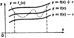
For simplicity of notation we suppose the exponential family is regular, so $\boldsymbol{\Theta}$ is open, but the results hold for any full family if $\boldsymbol{\Theta}$ is only restricted to its interior. Proposition $3.10$ showed that the log likelihood function is strictly concave and therefore has a unique maximum, corresponding to a unique root of the likelihood equations, provided there is a (finite) maximal value. We have seen examples in Chapter 3 of likelihoods without a finite maximum, for example in the binomial and Poisson families. We shall here first show that if we have a sample of size $n$ from a regular exponential family, the risk for such an event tends to zero with increasing $n$, and the MLE $\hat{\boldsymbol{\theta}}$ approaches the true $\boldsymbol{\theta}$, i.e. $\hat{\boldsymbol{\theta}}$ is a consistent estimator. The next step, to an asymptotic Gaussian distribution of $\hat{\boldsymbol{\theta}}$, is not big.
We shall use the following notation. Let $t(y)$ be the canonical statistic for a single observation, and $t_{n}=\sum_{i} t\left(y_{i}\right)$ the corresponding canonical statistic for the whole sample. Let $\mu_{t}(\theta)=E_{\theta}{t(y)}=E_{\theta}\left{t_{n} / n\right}$, i.e. the mean value per observational unit. The one-to-one canonical and mean-
value parameterizations by $\boldsymbol{\theta}$ and $\boldsymbol{\mu}$ are related by $\hat{\theta}(\boldsymbol{t})=\boldsymbol{\mu}^{-1}(\boldsymbol{t})$, and for a regular family both $\Theta$ and $\boldsymbol{\mu}(\boldsymbol{\Theta})$ are open sets in $\mathbb{R}^{k}$, where $k=\operatorname{dim} \theta$.
The existence and consistency of the MLE is essentially only a simple application of the law of large numbers under the mean value parameterization (when the MLE is $\hat{\mu}{t}=\boldsymbol{t}{n} / n$ ), followed by a reparameterization. In an analogous way, asymptotic normality of the MLE follows from the central limit theorem applied on $\hat{\mu}_{t}$. However, we will also indicate stronger versions of these results, utilizing more of the exponential family structure.
统计代写|统计模型作业代写Statistical Modelling代考|Existence and consistency of the MLE of θ
For a sample of size n from a regular exponential family, and for any $\boldsymbol{\theta} \in \boldsymbol{\Theta}$,
$$
\operatorname{Pr}\left{\hat{\boldsymbol{\theta}}\left(\boldsymbol{t}{n} / n\right) \text { exists; } \boldsymbol{\theta}\right} \rightarrow 1 \text { as } n \rightarrow \infty, $$ and furthermore, $$ \hat{\boldsymbol{\theta}}\left(\boldsymbol{t}{n} / n\right) \rightarrow \boldsymbol{\theta} \text { in probability as } n \rightarrow \infty
$$
These convergences are uniform on compact subsets of $\Theta$.
Proof By the (weak) law of large numbers (Khinchine version), $t_{n} / n \rightarrow$ $\boldsymbol{\mu}{t}\left(=\boldsymbol{\mu}{t}(\boldsymbol{\theta})\right)$ in probability as $n \rightarrow \infty$. More precisely expressed, for any fixed $\delta>0$,
$$
\operatorname{Pr}\left{\left|\boldsymbol{t}{n} / n-\boldsymbol{\mu}{t}\right|<\delta\right} \rightarrow 1 $$ Note that as soon as $\delta>0$ is small enough, the $\delta$-neighbourhood (4.1) of $\boldsymbol{\mu}{t}$ is wholly contained in the open set $\boldsymbol{\mu}(\boldsymbol{\Theta})$, and that $\boldsymbol{t}{n} / n$ is identical with the MLE $\hat{\boldsymbol{\mu}}{t}$. This is the existence and consistency result for the MLE of the mean value parameter, $\hat{\boldsymbol{\mu}}{t}$. Next we transform this to a result for $\hat{\boldsymbol{\theta}}$ in $\boldsymbol{\Theta}$.
Consider an open $\delta^{\prime}$-neighbourhood of $\theta$. For $\delta^{\prime}>0$ small enough, it is wholly within the open set $\boldsymbol{\Theta}$. There the image function $\boldsymbol{\mu}{t}(\boldsymbol{\theta})$ is welldefined, and the image of the $\delta^{\prime}$-neighbourhood of $\theta$ is an open neighbourhood of $\boldsymbol{\mu}(\boldsymbol{\theta})$ in $\boldsymbol{\mu}(\boldsymbol{\Theta})$ (since $\hat{\boldsymbol{\theta}}=\boldsymbol{\mu}{t}^{-1}$ is a continuous function). Inside that open neighbourhood we can always find (for some $\delta>0$ ) an open $\delta$ neighbourhood of type (4.1), whose probability goes to 1 . Thus, the probability for $\hat{\theta}\left(t_{n} / n\right)$ to be in the $\delta^{\prime}$-neighbourhood of $\theta$ also goes to 1 . This shows the asymptotic existence and consistency of $\hat{\boldsymbol{\theta}}$ for any fixed $\boldsymbol{\theta}$ in $\boldsymbol{\Theta}$.
Finally, this can be strengthened (Martin-Löf, 1970) to uniform convergence on compact subsets of the parameter space $\Theta$. Specifically, Chebyshev’s inequality can be used to give a more explicit upper bound of order $1 / n$ to the complementary probability, $\operatorname{Pr}\left{\left|t_{n} / n-\mu_{t}(\theta)\right| \geq \delta\right}$, proportional to $\operatorname{var}_{t}(\theta)$, that is bounded on compact subsets of $\boldsymbol{\Theta}$, since it is a continuous function of $\theta$. Details are omitted.
统计代写|统计模型作业代写Statistical Modelling代考|Uniform convergence on compacts
General results tells that under a set of suitable regularity conditions, the MLE is correspondingly asymptotically normally distributed as $n \rightarrow \infty$, but with the asymptotic variance expressed as being the inverse of the Fisher information. First note that when we are in a regular exponential family, we require no additional regularity conditions. Secondly, the variance $\operatorname{var}\left(\boldsymbol{t}{n} / n\right)=\operatorname{var}(t) / n$ for $\hat{\boldsymbol{\mu}}{\boldsymbol{t}}$ is precisely the inverse of the Fisher information matrix for $\mu_{t}$ (Proposition $\left.3.15\right)$, and unless $\psi\left(\mu_{t}\right)$ is of lower dimension than $\mu_{t}$ itself, the variance formula in Proposition $4.3$ can alternatively be obtained from $\operatorname{var}(t)$ by use of the Reparameterization lemma (Proposition 3.14). When $\psi$ and $\boldsymbol{\mu}{t}$ are not one-to-one, but $\operatorname{dim} \psi\left(\boldsymbol{\mu}{t}\right)<$ $\operatorname{dim} \mu_{t}$, e.g. $\psi$ a subvector of $\mu_{t}$, the theory of profile likelihoods (Section 3.3.4) can be useful, yielding correct formulas expressed in Fisher information terms. In a concrete situation we are of course free to calculate the estimator variance directly from the explicit form of $\hat{\psi}$. In any case, a conditional inference approach, eliminating nuisance parameters (Section $3.5)$, should also be considered. Asymptotically, however, we should not expect the conditional and unconditional results to differ, unless the nuisance parameters are incidental and increase in number with $n$, as in Exercise 3.16.
Note the special case of the canonical parameterization, with $\boldsymbol{\theta}$ as canonical parameter for the distribution of the single observation $(n=1)$. For this parameter, the asymptotic variance of the MLE is $\operatorname{var}(t)^{-1} / n$, where $t$ is the single observation statistic. This is the special case of Proposition $4.3$ for which
$$
\left(\frac{\partial \psi}{\partial \mu_{t}}\right)=\left(\frac{\partial \theta}{\partial \mu_{t}}\right)=\left(\frac{\partial \mu_{t}}{\partial \theta}\right)^{-1}=\operatorname{var}{\theta}(t)^{-1} $$ Like in the general large sample statistical theory, we may use the result of Proposition $4.3$ to construct asymptotically correct confidence regions. For example, expressed for the canonical parameter $\boldsymbol{\theta}$, it follows from Proposition $4.3$ that the quadratic form in $\hat{\theta}$, $$ Q(\boldsymbol{\theta})=n(\hat{\boldsymbol{\theta}}-\boldsymbol{\theta})^{T} \operatorname{var}{\theta}(\boldsymbol{t})(\hat{\boldsymbol{\theta}}-\boldsymbol{\theta})
$$

统计模型代考
统计代写|统计模型作业代写Statistical Modelling代考|Large Sample Asymptotics
为了符号的简单,我们假设指数族是规则的,所以θ是开放的,但结果适用于任何完整的家庭,如果θ仅限于其内部。主张3.10表明对数似然函数是严格凹的,因此具有唯一的最大值,对应于似然方程的唯一根,前提是存在(有限)最大值。我们已经在第 3 章中看到了没有有限最大值的可能性的例子,例如在二项式和泊松族中。我们将在这里首先证明,如果我们有一个大小为n从正则指数族中,此类事件的风险随着增加而趋于零n, 和 MLEθ^接近真实θ, IEθ^是一致的估计量。下一步,渐近高斯分布θ^,不大。
我们将使用以下符号。让吨(是)是单个观察的典型统计量,并且吨n=∑一世吨(是一世)整个样本的相应规范统计量。让\mu_{t}(\theta)=E_{\theta}{t(y)}=E_{\theta}\left{t_{n} / n\right}\mu_{t}(\theta)=E_{\theta}{t(y)}=E_{\theta}\left{t_{n} / n\right},即每个观测单位的平均值。一对一的规范和平均
值参数化θ和μ与θ^(吨)=μ−1(吨),对于普通家庭来说θ和μ(θ)是开集在Rķ, 在哪里ķ=暗淡θ.
MLE的存在性和一致性本质上只是在均值参数化下大数定律的简单应用(当MLE为$\hat{\mu} {t}=\boldsymbol{t} {n} / n),F这ll这在和db是一种r和p一种r一种米和吨和r一世和一种吨一世这n.一世n一种n一种n一种l这G这在s在一种是,一种s是米p吨这吨一世Cn这r米一种l一世吨是这F吨H和米大号和F这ll这在sFr这米吨H和C和n吨r一种ll一世米一世吨吨H和这r和米一种ppl一世和d这n\hat{\mu}_{t}$。但是,我们还将使用更多的指数族结构来指示这些结果的更强版本。
统计代写|统计模型作业代写Statistical Modelling代考|Existence and consistency of the MLE of θ
对于来自正则指数族的大小为 n 的样本,并且对于任何θ∈θ,
\operatorname{Pr}\left{\hat{\boldsymbol{\theta}}\left(\boldsymbol{t}{n} / n\right) \text { 存在;} \boldsymbol{\theta}\right} \rightarrow 1 \text { as } n \rightarrow \infty,\operatorname{Pr}\left{\hat{\boldsymbol{\theta}}\left(\boldsymbol{t}{n} / n\right) \text { 存在;} \boldsymbol{\theta}\right} \rightarrow 1 \text { as } n \rightarrow \infty,此外,θ^(吨n/n)→θ 概率为 n→∞
这些收敛在紧凑子集上是一致的θ.
证明由(弱)大数定律(Khinchin 版本),吨n/n→ μ吨(=μ吨(θ))概率为n→∞. 更准确地说,对于任何固定的d>0,
\operatorname{Pr}\left{\left|\boldsymbol{t}{n} / n-\boldsymbol{\mu}{t}\right|<\delta\right} \rightarrow 1\operatorname{Pr}\left{\left|\boldsymbol{t}{n} / n-\boldsymbol{\mu}{t}\right|<\delta\right} \rightarrow 1请注意,只要d>0足够小,则d- 邻里(4.1)μ吨完全包含在开集中μ(θ), 然后吨n/n与 MLE 相同μ^吨. 这是均值参数的 MLE 的存在性和一致性结果,μ^吨. 接下来我们将其转换为结果θ^在θ.
考虑一个开放的d′- 邻里θ. 为了d′>0足够小,它完全在开集中θ. 有图像功能μ吨(θ)定义明确,并且图像d′- 邻里θ是一个开放的邻域μ(θ)在μ(θ)(自从θ^=μ吨−1是一个连续函数)。在那个开放的社区里,我们总能找到(对于某些人来说d>0) 一个开放的d类型 (4.1) 的邻域,其概率为 1 。因此,概率为θ^(吨n/n)在d′- 邻里θ也去 1 。这说明了渐近存在性和一致性θ^对于任何固定θ在θ.
最后,这可以得到加强(Martin-Löf,1970)以在参数空间的紧凑子集上均匀收敛θ. 具体来说,切比雪夫不等式可用于给出更明确的阶数上限1/n到互补概率,\operatorname{Pr}\left{\left|t_{n} / n-\mu_{t}(\theta)\right| \geq \delta\right}\operatorname{Pr}\left{\left|t_{n} / n-\mu_{t}(\theta)\right| \geq \delta\right}, 与曾是吨(θ), 是有界的紧子集θ, 因为它是一个连续函数θ. 细节省略。
统计代写|统计模型作业代写Statistical Modelling代考|Uniform convergence on compacts
一般结果表明,在一组合适的正则性条件下,MLE 相应地渐近正态分布为n→∞,但渐近方差表示为 Fisher 信息的倒数。首先请注意,当我们在正则指数族中时,我们不需要额外的正则条件。其次,方差曾是(吨n/n)=曾是(吨)/n为了μ^吨正好是 Fisher 信息矩阵的逆μ吨(主张3.15), 除非ψ(μ吨)比μ吨本身,命题中的方差公式4.3也可以从曾是(吨)通过使用重新参数化引理(命题 3.14)。什么时候ψ和μ吨不是一对一的,而是暗淡ψ(μ吨)< 暗淡μ吨,例如ψ的子向量μ吨,轮廓似然理论(第 3.3.4 节)可能很有用,可以产生用 Fisher 信息项表示的正确公式。在具体情况下,我们当然可以直接从ψ^. 在任何情况下,条件推理方法,消除讨厌的参数(第3.5), 也应该考虑。然而,渐近地,我们不应该期望有条件和无条件的结果会有所不同,除非令人讨厌的参数是偶然的并且随着数量的增加而增加n,如练习 3.16 中所示。
请注意规范参数化的特殊情况,其中θ作为单一观测值分布的规范参数(n=1). 对于该参数,MLE 的渐近方差为曾是(吨)−1/n, 在哪里吨是单一观察统计量。这是命题的特例4.3为此
(∂ψ∂μ吨)=(∂θ∂μ吨)=(∂μ吨∂θ)−1=曾是θ(吨)−1就像在一般的大样本统计理论中,我们可以使用 Proposition 的结果4.3构造渐近正确的置信区域。例如,表示为规范参数θ, 它来自命题4.3二次形式在θ^,问(θ)=n(θ^−θ)吨曾是θ(吨)(θ^−θ)

统计代写请认准statistics-lab™. statistics-lab™为您的留学生涯保驾护航。
金融工程代写
金融工程是使用数学技术来解决金融问题。金融工程使用计算机科学、统计学、经济学和应用数学领域的工具和知识来解决当前的金融问题,以及设计新的和创新的金融产品。
非参数统计代写
非参数统计指的是一种统计方法,其中不假设数据来自于由少数参数决定的规定模型;这种模型的例子包括正态分布模型和线性回归模型。
广义线性模型代考
广义线性模型(GLM)归属统计学领域,是一种应用灵活的线性回归模型。该模型允许因变量的偏差分布有除了正态分布之外的其它分布。
术语 广义线性模型(GLM)通常是指给定连续和/或分类预测因素的连续响应变量的常规线性回归模型。它包括多元线性回归,以及方差分析和方差分析(仅含固定效应)。
有限元方法代写
有限元方法(FEM)是一种流行的方法,用于数值解决工程和数学建模中出现的微分方程。典型的问题领域包括结构分析、传热、流体流动、质量运输和电磁势等传统领域。
有限元是一种通用的数值方法,用于解决两个或三个空间变量的偏微分方程(即一些边界值问题)。为了解决一个问题,有限元将一个大系统细分为更小、更简单的部分,称为有限元。这是通过在空间维度上的特定空间离散化来实现的,它是通过构建对象的网格来实现的:用于求解的数值域,它有有限数量的点。边界值问题的有限元方法表述最终导致一个代数方程组。该方法在域上对未知函数进行逼近。[1] 然后将模拟这些有限元的简单方程组合成一个更大的方程系统,以模拟整个问题。然后,有限元通过变化微积分使相关的误差函数最小化来逼近一个解决方案。
tatistics-lab作为专业的留学生服务机构,多年来已为美国、英国、加拿大、澳洲等留学热门地的学生提供专业的学术服务,包括但不限于Essay代写,Assignment代写,Dissertation代写,Report代写,小组作业代写,Proposal代写,Paper代写,Presentation代写,计算机作业代写,论文修改和润色,网课代做,exam代考等等。写作范围涵盖高中,本科,研究生等海外留学全阶段,辐射金融,经济学,会计学,审计学,管理学等全球99%专业科目。写作团队既有专业英语母语作者,也有海外名校硕博留学生,每位写作老师都拥有过硬的语言能力,专业的学科背景和学术写作经验。我们承诺100%原创,100%专业,100%准时,100%满意。
随机分析代写
随机微积分是数学的一个分支,对随机过程进行操作。它允许为随机过程的积分定义一个关于随机过程的一致的积分理论。这个领域是由日本数学家伊藤清在第二次世界大战期间创建并开始的。
时间序列分析代写
随机过程,是依赖于参数的一组随机变量的全体,参数通常是时间。 随机变量是随机现象的数量表现,其时间序列是一组按照时间发生先后顺序进行排列的数据点序列。通常一组时间序列的时间间隔为一恒定值(如1秒,5分钟,12小时,7天,1年),因此时间序列可以作为离散时间数据进行分析处理。研究时间序列数据的意义在于现实中,往往需要研究某个事物其随时间发展变化的规律。这就需要通过研究该事物过去发展的历史记录,以得到其自身发展的规律。
回归分析代写
多元回归分析渐进(Multiple Regression Analysis Asymptotics)属于计量经济学领域,主要是一种数学上的统计分析方法,可以分析复杂情况下各影响因素的数学关系,在自然科学、社会和经济学等多个领域内应用广泛。
MATLAB代写
MATLAB 是一种用于技术计算的高性能语言。它将计算、可视化和编程集成在一个易于使用的环境中,其中问题和解决方案以熟悉的数学符号表示。典型用途包括:数学和计算算法开发建模、仿真和原型制作数据分析、探索和可视化科学和工程图形应用程序开发,包括图形用户界面构建MATLAB 是一个交互式系统,其基本数据元素是一个不需要维度的数组。这使您可以解决许多技术计算问题,尤其是那些具有矩阵和向量公式的问题,而只需用 C 或 Fortran 等标量非交互式语言编写程序所需的时间的一小部分。MATLAB 名称代表矩阵实验室。MATLAB 最初的编写目的是提供对由 LINPACK 和 EISPACK 项目开发的矩阵软件的轻松访问,这两个项目共同代表了矩阵计算软件的最新技术。MATLAB 经过多年的发展,得到了许多用户的投入。在大学环境中,它是数学、工程和科学入门和高级课程的标准教学工具。在工业领域,MATLAB 是高效研究、开发和分析的首选工具。MATLAB 具有一系列称为工具箱的特定于应用程序的解决方案。对于大多数 MATLAB 用户来说非常重要,工具箱允许您学习和应用专业技术。工具箱是 MATLAB 函数(M 文件)的综合集合,可扩展 MATLAB 环境以解决特定类别的问题。可用工具箱的领域包括信号处理、控制系统、神经网络、模糊逻辑、小波、仿真等。