如果你也在 怎样代写蒙特卡洛方法Monte Carlo method这个学科遇到相关的难题,请随时右上角联系我们的24/7代写客服。
蒙特卡洛方法,或称蒙特卡洛实验,是一类广泛的计算算法,依靠重复随机抽样来获得数值结果。其基本概念是利用随机性来解决原则上可能是确定性的问题。
statistics-lab™ 为您的留学生涯保驾护航 在代写蒙特卡洛方法Monte Carlo method方面已经树立了自己的口碑, 保证靠谱, 高质且原创的统计Statistics代写服务。我们的专家在代写蒙特卡洛方法Monte Carlo method代写方面经验极为丰富,各种代写蒙特卡洛方法Monte Carlo method相关的作业也就用不着说。
我们提供的蒙特卡洛方法Monte Carlo method及其相关学科的代写,服务范围广, 其中包括但不限于:
- Statistical Inference 统计推断
- Statistical Computing 统计计算
- Advanced Probability Theory 高等概率论
- Advanced Mathematical Statistics 高等数理统计学
- (Generalized) Linear Models 广义线性模型
- Statistical Machine Learning 统计机器学习
- Longitudinal Data Analysis 纵向数据分析
- Foundations of Data Science 数据科学基础
统计代写|蒙特卡洛方法代写Monte Carlo method代考|Definition of Models for Emission, Absorption
A surface is formally defined in Section $1.4$ as the interface between two regions of space having different optical properties, where the optical properties in question are the refractive and absorptive indices $n$ and $k$. We distinguish between these two properties and the models used to characterize the interaction between thermal radiation and surfaces. We are now in a position to elaborate on the definition and use of the surface
interaction models for emission, reflection, and absorption introduced in Chapter $1 .$
We define the directional spectral emissivity $\varepsilon(\lambda, T, \vartheta, \varphi)$ as the ratio of the spectral intensity of emission from a real body in direction $(\vartheta, \varphi)$ to the spectral intensity of a blackbody at the same temperature,
$$
\varepsilon(\lambda, T, \vartheta, \varphi) \equiv \frac{i_{\lambda, e}(\lambda, T, \vartheta, \varphi)}{i_{b \lambda}(\lambda, T)}
$$
Note that the symbol for the directional spectral emissivity can also be written $\varepsilon_{\lambda}^{\prime}(T)$, where the prime $\left({ }^{\prime}\right)$ indicates directionality and the subscript $\lambda$ identifies the model as spectral.
The directional total emissivity of a surface is then related to the directional spectral emissivity according to
$$
\varepsilon^{\prime}(T)=\varepsilon(T, \vartheta, \varphi)=\frac{\int_{\lambda=0}^{\omega} \varepsilon(\lambda, T, \vartheta, \varphi) i_{b \lambda}(\lambda, T) d \lambda}{\int_{\lambda=0}^{\infty} i_{b \lambda}(\lambda, T) d \lambda} .
$$
We know that the denominator is $\sigma T^{4} / \pi$, so Eq. (2.31) can be rewritten
$$
\varepsilon^{\prime}(T)=\varepsilon(T, \vartheta, \varphi)=\frac{\pi}{\sigma T^{4}} \int_{\lambda=0}^{\infty} \varepsilon(\lambda, T, \vartheta, \varphi) i_{b \lambda}(\lambda, T) d \lambda .
$$
A surface is said to be gray in a given direction $\left(\vartheta_{1}, \varphi_{1}\right)$ if the directional spectral emissivity is independent of wavelength in that direction. Equation (2.32) then defines a gray equivalent directional emissivity for spectral surfaces. The spectral intensities of a blackbody, a graybody, and a hypothetical real surface, all at $6000 \mathrm{~K}$, are compared in Figure $2.11$.
统计代写|蒙特卡洛方法代写Monte Carlo method代考|Introduction to the Radiation Behavior of Surfaces
The primary surface conditions that influence the radiation behavior of a solid surfacé ăré its bulk êlectricall propertiês (èléctrical conductor or non-conductor), its topography (smooth, polished, sanded, sand blasted, turned, lapped, honed, ground, peened, etc.), its chemical condition (reduced, oxidized, anodized, galvanized, etc.), its degree of contamination (clean or dirty, dusty, dry or oily, etc.), and its surface grain structure (annealed, cold rolled, hot rolled, etc.). Surfaces may also be painted, sputter coated, or evaporation coated to enhance or diminish emission, absorption, or reflection or to bias directionality and/or wavelength dependence. In addition, all surface preparations are subject to damage and aging. The result is a bewilderingly subjective array of adjectives, often open to interpretation, which renders effective communication between designers and modelers difficult if not impossible. Still, it is imperative, once a project moves out of the preliminary design phase, that engineers charged with performance modeling have access to accurate models for surface radiation behavior. In the extreme this often requires a surface characterization campaign, typically based on measurement of the bidirectional spectral reflectivity of key surfaces. The following brief review is intended as a guide to the reader tasked with formulating surface radiation behavior models, a topic treated in more detail in Chapter $4 .$
Maxwell’s Equations [10],
$$
\nabla \times \boldsymbol{H}=\varepsilon_{0} \frac{\partial \boldsymbol{E}}{\partial t}+\frac{\boldsymbol{E}}{r_{e}}
$$
$$
\begin{gathered}
\nabla \times \boldsymbol{E}=-\mu_{0} \frac{\partial \boldsymbol{H}}{\partial t} \
\nabla \cdot \boldsymbol{E}=\frac{\rho_{e}}{\varepsilon} \
\nabla \cdot \boldsymbol{H}=0
\end{gathered}
$$
are the point of departure for understanding the interaction of EM radiation with a surface. In Eqs. (2.62) to (2.65), $\boldsymbol{H}\left(\mathrm{Am}^{-1}\right)$ is the magnetic field strength, $\mathrm{E}\left(\mathrm{V} \mathrm{m}^{-1}\right)$ is the electric field strength, $\varepsilon_{0}=8.854 \mathrm{C}^{2} / \mathrm{N} \cdot \mathrm{m}^{2}$ is the permittivity of free space, $r_{e}(\Omega-\mathrm{m})$ is the electrical resistivity, $\rho_{e}\left(\mathrm{C} \mathrm{m}^{-3}\right)$ is the electric charge density, and $\mu_{0}=4 \pi \times 10^{-7} \mathrm{~N} \mathrm{~A}^{-2}$ is the magnetic permeability. These celebrated equations were formulated in 1864 by the British physicist and mathematician James Clerk Maxwell, who synthesized them from already known relationships between electricity and magnetism. Their solution permitted for the first time the theoretical calculation (see Problem 2.7) of the already known speed of light in a vacuum, thereby removing any doubt as to their validity.
统计代写|蒙特卡洛方法代写Monte Carlo method代考|Radiation Behavior of Surfaces Composed
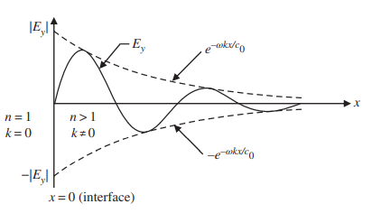
In the following paragraphs we consider the two limiting cases in which a monochromatic EM wave is incident to the plane interface separating two ideal regions. In the first extreme, the wave passes from a dielectric whose optical properties are $n_{1}$ and $k_{1}=0\left(r_{e} \rightarrow \infty\right)$ into another dielectric whose optical properties are $n_{2}$ and $k_{2}=0$; in the second extreme, the wave passes from a dielectric whose optical properties are $n_{1}$ and $k_{1}=0$ into an electrical conductor, or metal, whose optical properties are $n_{2}$ and $k_{2} \neq 0$
The case of a smooth plane interface between two dielectrics with $n_{2}>n_{1}$ is illustrated in Figure 2.19. In the figure $\boldsymbol{E}_{p, i}$ represents the
eléctric component of a transverse-magnetic (TM), p-polarized, monochromatic electromagnetic wave incident to the interface, or surface. The arrows labeled “Incident,” “Reflected,” and “Transmitted” can be thought of as “rays,” in which case the lines passing normal to the rays indicate wavefronts separated by a distance $\lambda$. Following convention, the subscript ” $p$ ” is used to remind us that the electric field vector in this case lies in the plane of incidence, the plane containing both the incident ray and the unit normal vector $\boldsymbol{n}=-i$. Without loss of generality we consider only the real part of the incident electric field,
$$
\operatorname{Re}\left[E_{p, i}\right]=\left|E_{p, i}\right| \cos \left[\omega\left(\frac{n_{1} x^{\prime}}{c_{0}}-t\right)\right],
$$
where $\omega=2 \pi c_{0} / \lambda$ and $x^{\prime}=y / \sin \vartheta_{i}$. This is equivalent to assuming that the phase angle of the incident wave, $\phi_{i}=\tan ^{-1}\left[\operatorname{Im}\left(E_{p, i}\right) / \operatorname{Re}\left(E_{p, i}\right)\right]$, is zero.
Careful consideration of Figure $2.19$ reveals that the $y$-component (parallel to the interface) of the electric field above the interface (region 1) is
$$
\begin{aligned}
\left|E_{y, 1}\right|=&\left|E_{p, i}\right| \cos \vartheta_{i} \cos \left[\omega\left(\frac{n_{1} y / \sin \vartheta_{i}}{c_{0}}-t\right)\right] \
&-\left|E_{p, r}\right| \cos \vartheta_{r} \cos \left[\omega\left(\frac{n_{1} y / \sin \vartheta_{r}}{c_{0}}-t\right)\right]
\end{aligned}
$$
and the $y$-component below the interface (region 2) is
$$
\left|E_{y, 2}\right|=\left|E_{p, t}\right| \cos \vartheta_{t} \cos \left[\omega\left(\frac{n_{2} y / \sin \vartheta_{t}}{c_{0}}-t\right)\right] .
$$
蒙特卡洛方法代考
统计代写|蒙特卡洛方法代写Monte Carlo method代考|Definition of Models for Emission, Absorption
表面在第 部分正式定义1.4作为具有不同光学特性的两个空间区域之间的界面,其中所讨论的光学特性是折射率和吸收指数n和ķ. 我们区分这两个属性和用于表征热辐射和表面之间相互作用的模型。我们现在可以详细说明表面的定义和使用
本章介绍的发射、反射和吸收的相互作用模型1.
我们定义了方向光谱发射率e(λ,吨,ϑ,披)作为来自真实物体的发射光谱强度在方向上的比率(ϑ,披)为相同温度下黑体的光谱强度,
e(λ,吨,ϑ,披)≡一世λ,和(λ,吨,ϑ,披)一世bλ(λ,吨)
请注意,方向光谱发射率的符号也可以写成eλ′(吨), 其中素数(′)指示方向性和下标λ将模型标识为光谱。
然后,表面的定向总发射率与定向光谱发射率相关,根据
e′(吨)=e(吨,ϑ,披)=∫λ=0ωe(λ,吨,ϑ,披)一世bλ(λ,吨)dλ∫λ=0∞一世bλ(λ,吨)dλ.
我们知道分母是σ吨4/圆周率,所以方程。(2.31) 可以改写
e′(吨)=e(吨,ϑ,披)=圆周率σ吨4∫λ=0∞e(λ,吨,ϑ,披)一世bλ(λ,吨)dλ.
表面在给定方向上是灰色的(ϑ1,披1)如果定向光谱发射率与该方向上的波长无关。然后等式 (2.32) 定义了光谱表面的灰色等效定向发射率。黑体、灰体和假设的真实表面的光谱强度,全部在6000 ķ, 比较如图2.11.
统计代写|蒙特卡洛方法代写Monte Carlo method代考|Introduction to the Radiation Behavior of Surfaces
影响固体表面辐射行为的主要表面条件包括其体积电性能(电导体或非导体)、其形貌(光滑、抛光、打磨、喷砂、车削、研磨、珩磨、研磨、喷丸等) .)、其化学状态(还原、氧化、阳极氧化、镀锌等)、污染程度(清洁或肮脏、多尘、干燥或油腻等)及其表面晶粒结构(退火、冷轧、热轧制等)。表面还可以被涂漆、溅射涂层或蒸发涂层以增强或减少发射、吸收或反射或偏向方向性和/或波长依赖性。此外,所有表面处理都会受到损坏和老化。结果是一系列令人眼花缭乱的主观形容词,通常可以解释,这使得设计师和建模师之间的有效沟通即使不是不可能也很困难。尽管如此,一旦项目退出初步设计阶段,负责性能建模的工程师必须能够获得准确的表面辐射行为模型。在极端情况下,这通常需要进行表面表征活动,通常基于对关键表面的双向光谱反射率的测量。以下简要回顾旨在为负责制定表面辐射行为模型的读者提供指南,该主题将在本章中更详细地讨论 负责性能建模的工程师可以获得表面辐射行为的准确模型。在极端情况下,这通常需要进行表面表征活动,通常基于对关键表面的双向光谱反射率的测量。以下简要回顾旨在为负责制定表面辐射行为模型的读者提供指南,该主题将在本章中更详细地讨论 负责性能建模的工程师可以获得表面辐射行为的准确模型。在极端情况下,这通常需要进行表面表征活动,通常基于对关键表面的双向光谱反射率的测量。以下简要回顾旨在为负责制定表面辐射行为模型的读者提供指南,该主题将在本章中更详细地讨论4.
麦克斯韦方程[10],
∇×H=e0∂和∂吨+和r和
∇×和=−μ0∂H∂吨 ∇⋅和=ρ和e ∇⋅H=0
是理解 EM 辐射与表面相互作用的出发点。在方程式中。(2.62)至(2.65),H(一个米−1)是磁场强度,和(在米−1)是电场强度,e0=8.854C2/ñ⋅米2是自由空间的介电常数,r和(Ω−米)是电阻率,ρ和(C米−3)是电荷密度,并且μ0=4圆周率×10−7 ñ 一个−2是磁导率。这些著名的方程是由英国物理学家和数学家詹姆斯·克拉克·麦克斯韦于 1864 年制定的,他从已知的电和磁之间的关系中合成了它们。他们的解决方案首次允许对已知的真空光速进行理论计算(参见问题 2.7),从而消除了对其有效性的任何怀疑。
统计代写|蒙特卡洛方法代写Monte Carlo method代考|Radiation Behavior of Surfaces Composed
在下面的段落中,我们考虑两种限制情况,其中单色 EM 波入射到分隔两个理想区域的平面界面。在第一个极端情况下,波从光学特性为n1和ķ1=0(r和→∞)进入另一个电介质,其光学特性是n2和ķ2=0; 在第二个极端中,波从其光学特性为n1和ķ1=0进入电导体或金属,其光学特性是n2和ķ2≠0
两种电介质之间的光滑平面界面的情况n2>n1如图 2.19 所示。图中和p,一世代表
入射到界面或表面的横磁 (TM)、p 极化、单色电磁波的电分量。标记为“入射”、“反射”和“透射”的箭头可以被认为是“射线”,在这种情况下,垂直于射线通过的线表示相隔一段距离的波前λ. 按照约定,下标“p”用来提醒我们,这种情况下的电场矢量位于入射平面,该平面同时包含入射光线和单位法向量n=−一世. 不失一般性,我们只考虑入射电场的实部,
回覆[和p,一世]=|和p,一世|因[ω(n1X′C0−吨)],
在哪里ω=2圆周率C0/λ和X′=是/罪ϑ一世. 这相当于假设入射波的相位角,φ一世=棕褐色−1[在里面(和p,一世)/回覆(和p,一世)], 为零。
仔细考虑图2.19揭示了是- 界面(区域 1)上方电场的分量(平行于界面)是
|和是,1|=|和p,一世|因ϑ一世因[ω(n1是/罪ϑ一世C0−吨)] −|和p,r|因ϑr因[ω(n1是/罪ϑrC0−吨)]
和是- 界面下方的组件(区域 2)是
|和是,2|=|和p,吨|因ϑ吨因[ω(n2是/罪ϑ吨C0−吨)].

统计代写请认准statistics-lab™. statistics-lab™为您的留学生涯保驾护航。
金融工程代写
金融工程是使用数学技术来解决金融问题。金融工程使用计算机科学、统计学、经济学和应用数学领域的工具和知识来解决当前的金融问题,以及设计新的和创新的金融产品。
非参数统计代写
非参数统计指的是一种统计方法,其中不假设数据来自于由少数参数决定的规定模型;这种模型的例子包括正态分布模型和线性回归模型。
广义线性模型代考
广义线性模型(GLM)归属统计学领域,是一种应用灵活的线性回归模型。该模型允许因变量的偏差分布有除了正态分布之外的其它分布。
术语 广义线性模型(GLM)通常是指给定连续和/或分类预测因素的连续响应变量的常规线性回归模型。它包括多元线性回归,以及方差分析和方差分析(仅含固定效应)。
有限元方法代写
有限元方法(FEM)是一种流行的方法,用于数值解决工程和数学建模中出现的微分方程。典型的问题领域包括结构分析、传热、流体流动、质量运输和电磁势等传统领域。
有限元是一种通用的数值方法,用于解决两个或三个空间变量的偏微分方程(即一些边界值问题)。为了解决一个问题,有限元将一个大系统细分为更小、更简单的部分,称为有限元。这是通过在空间维度上的特定空间离散化来实现的,它是通过构建对象的网格来实现的:用于求解的数值域,它有有限数量的点。边界值问题的有限元方法表述最终导致一个代数方程组。该方法在域上对未知函数进行逼近。[1] 然后将模拟这些有限元的简单方程组合成一个更大的方程系统,以模拟整个问题。然后,有限元通过变化微积分使相关的误差函数最小化来逼近一个解决方案。
tatistics-lab作为专业的留学生服务机构,多年来已为美国、英国、加拿大、澳洲等留学热门地的学生提供专业的学术服务,包括但不限于Essay代写,Assignment代写,Dissertation代写,Report代写,小组作业代写,Proposal代写,Paper代写,Presentation代写,计算机作业代写,论文修改和润色,网课代做,exam代考等等。写作范围涵盖高中,本科,研究生等海外留学全阶段,辐射金融,经济学,会计学,审计学,管理学等全球99%专业科目。写作团队既有专业英语母语作者,也有海外名校硕博留学生,每位写作老师都拥有过硬的语言能力,专业的学科背景和学术写作经验。我们承诺100%原创,100%专业,100%准时,100%满意。
随机分析代写
随机微积分是数学的一个分支,对随机过程进行操作。它允许为随机过程的积分定义一个关于随机过程的一致的积分理论。这个领域是由日本数学家伊藤清在第二次世界大战期间创建并开始的。
时间序列分析代写
随机过程,是依赖于参数的一组随机变量的全体,参数通常是时间。 随机变量是随机现象的数量表现,其时间序列是一组按照时间发生先后顺序进行排列的数据点序列。通常一组时间序列的时间间隔为一恒定值(如1秒,5分钟,12小时,7天,1年),因此时间序列可以作为离散时间数据进行分析处理。研究时间序列数据的意义在于现实中,往往需要研究某个事物其随时间发展变化的规律。这就需要通过研究该事物过去发展的历史记录,以得到其自身发展的规律。
回归分析代写
多元回归分析渐进(Multiple Regression Analysis Asymptotics)属于计量经济学领域,主要是一种数学上的统计分析方法,可以分析复杂情况下各影响因素的数学关系,在自然科学、社会和经济学等多个领域内应用广泛。
MATLAB代写
MATLAB 是一种用于技术计算的高性能语言。它将计算、可视化和编程集成在一个易于使用的环境中,其中问题和解决方案以熟悉的数学符号表示。典型用途包括:数学和计算算法开发建模、仿真和原型制作数据分析、探索和可视化科学和工程图形应用程序开发,包括图形用户界面构建MATLAB 是一个交互式系统,其基本数据元素是一个不需要维度的数组。这使您可以解决许多技术计算问题,尤其是那些具有矩阵和向量公式的问题,而只需用 C 或 Fortran 等标量非交互式语言编写程序所需的时间的一小部分。MATLAB 名称代表矩阵实验室。MATLAB 最初的编写目的是提供对由 LINPACK 和 EISPACK 项目开发的矩阵软件的轻松访问,这两个项目共同代表了矩阵计算软件的最新技术。MATLAB 经过多年的发展,得到了许多用户的投入。在大学环境中,它是数学、工程和科学入门和高级课程的标准教学工具。在工业领域,MATLAB 是高效研究、开发和分析的首选工具。MATLAB 具有一系列称为工具箱的特定于应用程序的解决方案。对于大多数 MATLAB 用户来说非常重要,工具箱允许您学习和应用专业技术。工具箱是 MATLAB 函数(M 文件)的综合集合,可扩展 MATLAB 环境以解决特定类别的问题。可用工具箱的领域包括信号处理、控制系统、神经网络、模糊逻辑、小波、仿真等。