statistics-lab™ 为您的留学生涯保驾护航 在代写运筹学operational research方面已经树立了自己的口碑, 保证靠谱, 高质且原创的统计Statistics代写服务。我们的专家在代写运筹学operational research代写方面经验极为丰富,各种代写运筹学operational research相关的作业也就用不着说。
我们提供的运筹学operational research及其相关学科的代写,服务范围广, 其中包括但不限于:
- Statistical Inference 统计推断
- Statistical Computing 统计计算
- Advanced Probability Theory 高等楖率论
- Advanced Mathematical Statistics 高等数理统计学
- (Generalized) Linear Models 广义线性模型
- Statistical Machine Learning 统计机器学习
- Longitudinal Data Analysis 纵向数据分析
- Foundations of Data Science 数据科学基础
统计代写|运筹学作业代写operational research代考|Concept of Transshipment Problem
The transshipment problem is an extension of the transportation problem. For the transportation problem, it is assumed that a commodity can only be shipped from an origin to a destination. In many real-life situations, it is also possible to distribute the commodity through the points of origins or through the points of destinations. Sometimes it might be advantageous to distribute a commodity from an origin to an intermediate, or transshipment, point before shipping it to a destination. The transshipment problem allows for these shipments.
The transshipment problem can be described as follows. A manufacturing company has a number of plants, each of which has a limited available capacity, $s_{i}$. After manufacturing, the semifinished products are delivered to the warehouses for final assembly and packaging. Finally, the finished products are shipped to the customers according to their requirements, $d_{j}$. The problem is how to fulfill each customer’s order while not exceeding the capacity of any plant at the minimum cost, $c_{i j \text { – }}$ The problem can be transformed as a conventional transportation model with $(n-b)$ origins and $(n-a)$ destinations, where $n$ is the total number of nodes in the network (i.e., total number of plants, warehouses, and customers), $a$ is the number of node that has supply only (or pure origin), and $b$ is the number of nodes that has demand only (or pure destination). Any node that has both supply and demand is referred to as a transshipment point. The unit transportation costs, $c_{i j}$ are often dependent on the travel distances from node $i$ to node $j$. It is assumed that the cost on a particular route of the network is directly proportional to the amount of products shipped on that route. If there is no route connecting node $i$ and node $j$-or arc $(i, j)$ does not exist-then the cost is considered $\infty$. The cost of delivering 1 unit of product from node $i$ to itself is 0 . By introducing decision variables $x_{i j}$ to represent the amount of product sent from node $i$ to node $j$, the transshipment model can be written as shown in Model 2.3.1.
统计代写|运筹学作业代写operational research代考|Example of Transshipment Problem
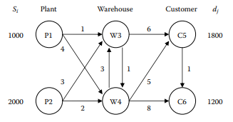
The following example, illustrated in Figure $2.12$, shows a transshipment problem. A manufacturing company has two plants. Plant 1 can produce up to 1000 units of products per day, whereas plant 2 can produce as many as 2000 units of products per day. Instead of shipping the products directly to its customers, each product must be distributed to a warehouse first. After assembling and packaging in the warehouses, the products are shipped to the customers. The demand amounts of customer 1 and customer 2 are 1800 and 1200 , respectively. The problem is how to fulfill each customer’s order
while not exceeding the capacity of any plant at the minimum cost, $c_{i \ddot{ }}$. Unit transportation costs, $c_{i j}$, are shown above the arcs (or arrows).
This transshipment model can be converted into a conventional transportation model with five origins (i.e., P1, P2, W3, W4, and C5) and four destinations (i.e., W3, W4, C5, and C6). The supplies of origins and the demands of destinations are computed as follows. For the five origins, each plant (i.e., $P 1$ and P2) will have a supply equal to its original supply, whereas each warehouse and the first customer (i.e., W3, W4, and C5) will have a supply equal to the total available supply. For the four destinations, each warehouse (i.e., W3 and W4) will have a demand equal to the total available supply. The first customer (i.e, C5) will have a demand equal to the summation of its original demand and total available supply, whereas the second customer (i.e., C6) will have a demand equal to its original demand. The reasons for adding the total available supply to the supply and demand at each transshipment point are to ensure that the total amount of products shipped through each transshipment point will not exceed the total available supply and to also balance the transportation model.
Table $2.5$ details this transshipment problem. Decision variables $x_{i j}$ represent the amount of the products delivered from origin $i$ to destination $j$. The demand of each destination, $d_{j}$, and the supply of each origin, $s_{j}$, are shown. The upperright corner of each cell in the tableau represents the unit transportation cost, $c_{i j}$. By introducing decision variables $x_{i j}$ to represent the shipment from origin $i$ to destination $j$, this transshipment problem can be formulated as shown in Model 2.3.2.
统计代写|运筹学作业代写operational research代考| SAS Code for Transshipment Problem
ORTRANS, explained in Section $2.1$ (see also program “sasor_2_3.sas”), is a macro that solves transportation problems, the objective of which is to yield the minimum cost of shipment through a transportation network to destinations. The transshipment problem is an extension of the transportation problem, hence the same macro can be used for this example.
The only difference is that in the transshipment tableau (Table $2.5$ ) some of the costs are set to be $\infty$. Hence in the dataset, we use a large number instead (e.g., $1 \mathrm{E} 10$, which is $10^{10}$ ) because using a large number forces the user to set a variable to 0 . However, such a practice introduces numerical instability, hence we added the code shown next in the program. This constraint explicity fixes the value of the corresponding variables to 0 .
con zero{c in CUSTOMERS, $s$ in SUPPLIERS : cost $[s, c]=1 E 10}$ :
$x[s, c]=0$;
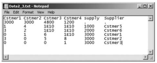
An example data file is seen in Figure 2.13.
Note that the following notations are used in this data file: Cstmer1 (W3), Cstmer2 (W4), Cstmer3 (C5), Cstmer4 (C6), Cstmer5 (P1), and Cstmer6 (P2).
Similar to Section 2.1, two parameters need to be set before calling the \%ortrans macro:
_data: Indicates the name and location of the data file (a text tab delimited file) and contains the cost matrix
_itle: Gives a title in the output of the SAS
运筹学代考
统计代写|运筹学作业代写operational research代考|Concept of Transshipment Problem
转运问题是运输问题的延伸。对于运输问题,假设商品只能从原产地运送到目的地。在许多现实生活中,还可以通过起点或通过目的地分配商品。有时,在将商品运送到目的地之前,将商品从原产地分发到中间或转运点可能是有利的。转运问题允许这些货物。
转运问题可以描述如下。一家制造公司有许多工厂,每个工厂都有有限的可用产能,s一世. 制造完成后,将半成品运送到仓库进行最终组装和包装。最后,根据客户的要求将成品运送给客户,dj. 问题是如何以最低成本完成每个客户的订单,同时不超过任何工厂的产能,C一世j – 该问题可以转化为传统的交通模型(n−b)起源和(n−一种)目的地,在哪里n是网络中的节点总数(即工厂、仓库和客户的总数),一种是仅具有供应(或纯来源)的节点数,并且b是仅具有需求(或纯目的地)的节点数。任何既有供给又有需求的节点称为转运点。单位运输成本,C一世j通常取决于到节点的行进距离一世到节点j. 假设网络特定路线的成本与该路线上运送的产品数量成正比。如果没有路由连接节点一世和节点j- 或弧(一世,j)不存在-则考虑成本∞. 从节点交付 1 单位产品的成本一世对自身是 0 。通过引入决策变量X一世j表示从节点发送的产品数量一世到节点j, 转运模型可写成模型 2.3.1 所示。
统计代写|运筹学作业代写operational research代考|Example of Transshipment Problem
下面的例子,如图2.12,表示转运问题。一家制造公司有两个工厂。工厂 1 每天最多可以生产 1000 件产品,而工厂 2 每天可以生产多达 2000 件产品。每个产品都必须先分发到仓库,而不是直接将产品运送给客户。在仓库组装和包装后,将产品运送给客户。客户 1 和客户 2 的需求量分别为 1800 和 1200 。问题是如何完成每个客户的订单
在不以最低成本超出任何工厂的产能的同时,C一世¨. 单位运输成本,C一世j, 显示在弧线(或箭头)上方。
这种转运模型可以转换为具有五个起点(即P1、P2、W3、W4 和C5)和四个目的地(即W3、W4、C5 和C6)的常规运输模型。来源地的供给和目的地的需求计算如下。对于五个起源,每个植物(即,磷1和 P2) 的供应量将等于其原始供应量,而每个仓库和第一个客户(即 W3、W4 和 C5)的供应量将等于总可用供应量。对于四个目的地,每个仓库(即 W3 和 W4)的需求量将等于总可用供应量。第一个客户(即 C5)的需求等于其原始需求和总可用供应的总和,而第二个客户(即 C6)的需求等于其原始需求。将可用供应总量添加到每个转运点的供需中的原因是为了确保通过每个转运点运输的产品总量不会超过可用供应总量,同时也是为了平衡运输模式。
桌子2.5详细说明了这个转运问题。决策变量X一世j代表从原产地交付的产品数量一世到目的地j. 每个目的地的需求,dj,以及每个来源的供应,sj, 显示。表格中每个单元格的右上角代表单位运输成本,C一世j. 通过引入决策变量X一世j代表从原产地发货一世到目的地j,这个转运问题可以表述为模型2.3.2。
统计代写|运筹学作业代写operational research代考| SAS Code for Transshipment Problem
ORTRANS,在章节中解释2.1(另见程序“sasor_2_3.sas”),是一个解决运输问题的宏,其目标是通过运输网络产生最小的运输成本到目的地。转运问题是运输问题的扩展,因此本例可以使用相同的宏。
唯一的区别是在转运画面(表2.5) 一些成本设定为∞. 因此,在数据集中,我们使用了一个很大的数字(例如,1和10,即1010) 因为使用大数会迫使用户将变量设置为 0 。但是,这种做法会引入数值不稳定,因此我们在程序中添加了接下来显示的代码。此约束明确地将相应变量的值固定为 0 。
客户中的 con zero{c,s在供应商中:成本[s, c]=1 E 10}[s, c]=1 E 10} :
X[s,C]=0;
示例数据文件如图 2.13 所示。
请注意,此数据文件中使用了以下符号:Cstmer1 (W3)、Cstmer2 (W4)、Cstmer3 (C5)、Cstmer4 (C6)、Cstmer5 (P1) 和 Cstmer6 (P2)。
与 2.1 节类似,在调用 \%ortrans 宏之前需要设置两个参数: _data
:指示数据文件的名称和位置(文本制表符分隔的文件)并包含成本矩阵
_itle:在输出中给出标题SAS 的

统计代写请认准statistics-lab™. statistics-lab™为您的留学生涯保驾护航。
金融工程代写
金融工程是使用数学技术来解决金融问题。金融工程使用计算机科学、统计学、经济学和应用数学领域的工具和知识来解决当前的金融问题,以及设计新的和创新的金融产品。
非参数统计代写
非参数统计指的是一种统计方法,其中不假设数据来自于由少数参数决定的规定模型;这种模型的例子包括正态分布模型和线性回归模型。
广义线性模型代考
广义线性模型(GLM)归属统计学领域,是一种应用灵活的线性回归模型。该模型允许因变量的偏差分布有除了正态分布之外的其它分布。
术语 广义线性模型(GLM)通常是指给定连续和/或分类预测因素的连续响应变量的常规线性回归模型。它包括多元线性回归,以及方差分析和方差分析(仅含固定效应)。
有限元方法代写
有限元方法(FEM)是一种流行的方法,用于数值解决工程和数学建模中出现的微分方程。典型的问题领域包括结构分析、传热、流体流动、质量运输和电磁势等传统领域。
有限元是一种通用的数值方法,用于解决两个或三个空间变量的偏微分方程(即一些边界值问题)。为了解决一个问题,有限元将一个大系统细分为更小、更简单的部分,称为有限元。这是通过在空间维度上的特定空间离散化来实现的,它是通过构建对象的网格来实现的:用于求解的数值域,它有有限数量的点。边界值问题的有限元方法表述最终导致一个代数方程组。该方法在域上对未知函数进行逼近。[1] 然后将模拟这些有限元的简单方程组合成一个更大的方程系统,以模拟整个问题。然后,有限元通过变化微积分使相关的误差函数最小化来逼近一个解决方案。
tatistics-lab作为专业的留学生服务机构,多年来已为美国、英国、加拿大、澳洲等留学热门地的学生提供专业的学术服务,包括但不限于Essay代写,Assignment代写,Dissertation代写,Report代写,小组作业代写,Proposal代写,Paper代写,Presentation代写,计算机作业代写,论文修改和润色,网课代做,exam代考等等。写作范围涵盖高中,本科,研究生等海外留学全阶段,辐射金融,经济学,会计学,审计学,管理学等全球99%专业科目。写作团队既有专业英语母语作者,也有海外名校硕博留学生,每位写作老师都拥有过硬的语言能力,专业的学科背景和学术写作经验。我们承诺100%原创,100%专业,100%准时,100%满意。
随机分析代写
随机微积分是数学的一个分支,对随机过程进行操作。它允许为随机过程的积分定义一个关于随机过程的一致的积分理论。这个领域是由日本数学家伊藤清在第二次世界大战期间创建并开始的。
时间序列分析代写
随机过程,是依赖于参数的一组随机变量的全体,参数通常是时间。 随机变量是随机现象的数量表现,其时间序列是一组按照时间发生先后顺序进行排列的数据点序列。通常一组时间序列的时间间隔为一恒定值(如1秒,5分钟,12小时,7天,1年),因此时间序列可以作为离散时间数据进行分析处理。研究时间序列数据的意义在于现实中,往往需要研究某个事物其随时间发展变化的规律。这就需要通过研究该事物过去发展的历史记录,以得到其自身发展的规律。
回归分析代写
多元回归分析渐进(Multiple Regression Analysis Asymptotics)属于计量经济学领域,主要是一种数学上的统计分析方法,可以分析复杂情况下各影响因素的数学关系,在自然科学、社会和经济学等多个领域内应用广泛。
MATLAB代写
MATLAB 是一种用于技术计算的高性能语言。它将计算、可视化和编程集成在一个易于使用的环境中,其中问题和解决方案以熟悉的数学符号表示。典型用途包括:数学和计算算法开发建模、仿真和原型制作数据分析、探索和可视化科学和工程图形应用程序开发,包括图形用户界面构建MATLAB 是一个交互式系统,其基本数据元素是一个不需要维度的数组。这使您可以解决许多技术计算问题,尤其是那些具有矩阵和向量公式的问题,而只需用 C 或 Fortran 等标量非交互式语言编写程序所需的时间的一小部分。MATLAB 名称代表矩阵实验室。MATLAB 最初的编写目的是提供对由 LINPACK 和 EISPACK 项目开发的矩阵软件的轻松访问,这两个项目共同代表了矩阵计算软件的最新技术。MATLAB 经过多年的发展,得到了许多用户的投入。在大学环境中,它是数学、工程和科学入门和高级课程的标准教学工具。在工业领域,MATLAB 是高效研究、开发和分析的首选工具。MATLAB 具有一系列称为工具箱的特定于应用程序的解决方案。对于大多数 MATLAB 用户来说非常重要,工具箱允许您学习和应用专业技术。工具箱是 MATLAB 函数(M 文件)的综合集合,可扩展 MATLAB 环境以解决特定类别的问题。可用工具箱的领域包括信号处理、控制系统、神经网络、模糊逻辑、小波、仿真等。