如果你也在 怎样代写金融统计Mathematics with Statistics for Finance G1GH这个学科遇到相关的难题,请随时右上角联系我们的24/7代写客服。
金融统计描述了应用数学和数学模型来解决金融问题。它有时被称为定量金融,金融工程,和计算金融。
statistics-lab™ 为您的留学生涯保驾护航 在代写金融统计Mathematics with Statistics for Finance G1GH方面已经树立了自己的口碑, 保证靠谱, 高质且原创的统计Statistics代写服务。我们的专家在代写金融统计Mathematics with Statistics for Finance G1GH方面经验极为丰富,各种代写金融统计Mathematics with Statistics for Finance G1GH相关的作业也就用不着说。
我们提供的金融统计Mathematics with Statistics for Finance G1GH及其相关学科的代写,服务范围广, 其中包括但不限于:
- Statistical Inference 统计推断
- Statistical Computing 统计计算
- Advanced Probability Theory 高等楖率论
- Advanced Mathematical Statistics 高等数理统计学
- (Generalized) Linear Models 广义线性模型
- Statistical Machine Learning 统计机器学习
- Longitudinal Data Analysis 纵向数据分析
- Foundations of Data Science 数据科学基础
统计代写|金融统计代写Mathematics with Statistics for Finance代考|SKEWNESS
The second central moment, variance, tells us how spread-out a random variable is around the mean. The third central moment tells us how symmetrical
the distribution is around the mean. Rather than working with the third central moment directly, by convention we first standardize the statistic. This standardized third central moment is known as skewness:
$$
\text { Skewness }=\frac{E\left[(X-\mu)^{3}\right]}{\sigma^{3}}
$$
where $\sigma$ is the standard deviation of $X$.
By standardizing the central moment, it is much easier to compare two random variables. Multiplying a random variable by a constant will not change the skewness.
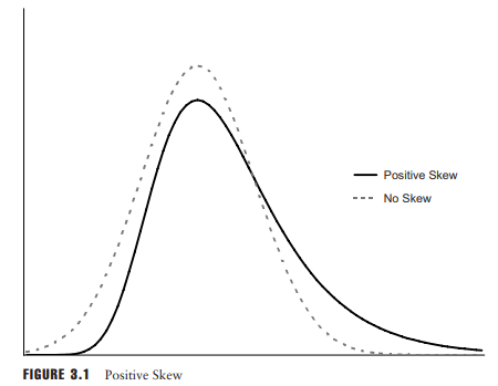
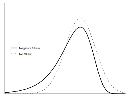
A random variable that is symmetrical about its mean will have zero skewness. If the skewness of the random variable is positive, we say that the random variable exhibits positive skew. Figures $3.1$ and $3.2$ show examples of positive and negative skewness.
Skewness is a very important concept in risk management. If the distributions of returns of two investments are the same in all respects, with the same mean and standard deviation but different skews, then the investment with more negative skew is generally considered to be more risky. Historical data suggest that many financial assets exhibit negative skew.
统计代写|金融统计代写Mathematics with Statistics for Finance代考|Negative Skew
As with variance, the equation for skewness differs depending on whether we are calculating the population skewness or the sample skewness. For the population statistic, the skewness of a random variable $X$, based on $n$ observations, $x_{1}, x_{2}, \ldots, x_{n}$, can be calculated as:
$$
\hat{s}=\sum_{i=1}^{n}\left(\frac{x_{i}-\mu}{\sigma}\right)^{3}
$$
where $\mu$ is the population mean and $\sigma$ is the population standard deviation. Similar to our calculation of sample variance, if we are calculating the sample skewness, there is going to be an overlap with the calculation of the sample mean and sample standard deviation. We need to correct for that. The sample skewness can be calculated as:
$$
\tilde{s}=\frac{n}{(n-1)(n-2)} \sum_{i=1}^{n}\left(\frac{x_{i}-\hat{\mu}}{\hat{\sigma}}\right)^{3}
$$
Based on Equation $3.20$ for variance, it is tempting to guess that the formula for the third central moment can be written simply in terms of $E\left[X^{3}\right]$ and $\mu$. Be careful, as the two sides of this equation are not equal:
$$
E\left[(X-\mu)^{k}\right] \neq E\left[X^{3}\right]-\mu^{3}
$$
The correct equation is:
$$
E\left[(X-\mu)^{3}\right]=E\left[X^{3}\right]-3 \mu \sigma^{2}-\mu^{3}
$$
统计代写|金融统计代写Mathematics with Statistics for Finance代考|KURTOSIS
The fourth central moment is similar to the second central moment, in that it tells us how spread-out a random variable is, but it puts more weight on extreme points. As with skewness, rather than working with the central moment directly, we typically work with a standardized statistic. This standardized fourth central moment is known as the kurtosis. For a random variable $X$, we can define the kurtosis as $K$, where:
$$
K=\frac{E\left[(X-\mu)^{4}\right]}{\sigma^{4}}
$$
where $\sigma$ is the standard deviation of $X$, and $\mu$ is its mean.
By standardizing the central moment, it is much easier to compare two random variables. As with skewness, multiplying a random variable by a constant will not change the kurtosis.
The following two populations have the same mean, variance, and skewness. The second population has a higher kurtosis.
Population 1: ${-17,-17,17,17}$
Population 2: ${-23,-7,7,23}$
Notice, to balance out the variance, when we moved the outer two points out six units, we had to move the inner two points in 10 units. Because the random variable with higher kurtosis has points further from the mean, we often refer to distribution with high kurtosis as fat-tailed. Figures $3.3$ and $3.4$ show examples of continuous distributions with high and low kurtosis.
Like skewness, kurtosis is an important concept in risk management. Many financial assets exhibit high levels of kurtosis. If the distribution of
returns of two assets have the same mean, variance, and skewness, but different kurtosis, then the distribution with the higher kurtosis will tend to have more extreme points, and be considered more risky.
As with variance and skewness, the equation for kurtosis differs depending on whether we are calculating the population kurtosis or the sample kurtosis. For the population statistic, the kurtosis of a random variable $X$ can be calculated as:
$$
\hat{K}=\sum_{i=1}^{n}\left(\frac{x_{i}-\mu}{\sigma}\right)^{4}
$$
where $\mu$ is the population mean and $\sigma$ is the population standard deviation. Similar to our calculation of sample variance, if we are calculating the sample kurtosis, there is going to be an overlap with the calculation of the sample mean and sample standard deviation. We need to correct for that. The sample kurtosis can be calculated as:
$$
\tilde{K}=\frac{n(n+1)}{(n-1)(n-2)(n-3)} \sum_{i=1}^{n}\left(\frac{x_{i}-\hat{\mu}}{\hat{\sigma}}\right)^{4}
$$
In the next chapter we will study the normal distribution, which has a kurtosis of 3 . Because normal distributions are so common, many people refer to “excess kurtosis,” which is simply the kurtosis minus 3 .
$$
K_{\text {excess }}=K-3
$$
In this way, the normal distribution has an excess kurtosis of 0 . Distributions with positive excess kurtosis are termed leptokurtotic. Distributions with negative excess kurtosis are termed platykurtotic. Be careful; by default, many applications calculate excess kurtosis.
When we are also estimating the mean and variance, calculating the sample excess kurtosis is somewhat more complicated than just subtracting 3. The correct formula is:
$$
\tilde{K}_{\text {excess }}=\tilde{K}-3 \frac{(n-1)^{2}}{(n-2)(n-3)}
$$
where $\tilde{K}$ is the sample kurtosis from Equation 3.46. As $n$ increases, the last term on the right-hand side converges to 3 .
金融统计代写
统计代写|金融统计代写Mathematics with Statistics for Finance代考|SKEWNESS
第二个中心矩,方差,告诉我们随机变量在均值附近的分布程度。第三个中心矩告诉我们如何对称
分布在均值附近。按照惯例,我们首先对统计数据进行标准化,而不是直接使用第三个中心矩。这个标准化的第三个中心矩称为偏度:
偏度 =和[(X−μ)3]σ3
在哪里σ是标准差X.
通过标准化中心矩,比较两个随机变量要容易得多。将随机变量乘以常数不会改变偏度。
一个关于其均值对称的随机变量将具有零偏度。如果随机变量的偏度为正,我们称随机变量呈现正偏度。数据3.1和3.2显示正偏度和负偏度的示例。
偏度是风险管理中一个非常重要的概念。如果两种投资的收益分布在所有方面都相同,均值和标准差相同,但偏度不同,则通常认为具有更大负偏度的投资风险更大。历史数据表明,许多金融资产呈现负偏斜。
统计代写|金融统计代写Mathematics with Statistics for Finance代考|Negative Skew
与方差一样,偏度方程的不同取决于我们计算的是总体偏度还是样本偏度。对于总体统计量,随机变量的偏度X, 基于n观察,X1,X2,…,Xn, 可以计算为:
s^=∑一世=1n(X一世−μσ)3
在哪里μ是总体均值和σ是总体标准差。与我们对样本方差的计算类似,如果我们在计算样本偏度,那么样本均值和样本标准差的计算将会有重叠。我们需要对此进行纠正。样本偏度可以计算为:
s~=n(n−1)(n−2)∑一世=1n(X一世−μ^σ^)3
基于方程3.20对于方差,很容易猜测第三个中心矩的公式可以简单地写成和[X3]和μ. 小心,因为这个等式的两边不相等:
和[(X−μ)ķ]≠和[X3]−μ3
正确的方程式是:
和[(X−μ)3]=和[X3]−3μσ2−μ3
统计代写|金融统计代写Mathematics with Statistics for Finance代考|KURTOSIS
第四中心矩与第二中心矩相似,它告诉我们随机变量的分散程度,但它更重视极值点。与偏度一样,我们通常不是直接使用中心矩,而是使用标准化的统计数据。这个标准化的第四中心矩称为峰度。对于随机变量X,我们可以将峰度定义为ķ, 在哪里:
ķ=和[(X−μ)4]σ4
在哪里σ是标准差X, 和μ是它的意思。
通过标准化中心矩,比较两个随机变量要容易得多。与偏度一样,将随机变量乘以常数不会改变峰度。
以下两个总体具有相同的均值、方差和偏度。第二个群体的峰度较高。
人口 1:−17,−17,17,17
人口 2:−23,−7,7,23
请注意,为了平衡方差,当我们将外部两个点移出 6 个单位时,我们必须将内部两个点移出 10 个单位。因为具有较高峰度的随机变量的点距均值较远,所以我们通常将具有高峰度的分布称为肥尾分布。数据3.3和3.4显示具有高峰度和低峰度的连续分布的示例。
像偏度一样,峰度是风险管理中的一个重要概念。许多金融资产表现出高水平的峰态。如果分布
两种资产的收益具有相同的均值、方差和偏度,但峰度不同,那么峰度较高的分布往往会出现更多的极值点,被认为风险更大。
与方差和偏度一样,峰度方程的不同取决于我们计算的是总体峰度还是样本峰度。对于总体统计量,随机变量的峰度X可以计算为:
ķ^=∑一世=1n(X一世−μσ)4
在哪里μ是总体均值和σ是总体标准差。与我们对样本方差的计算类似,如果我们在计算样本峰度,那么样本均值和样本标准差的计算将会有重叠。我们需要对此进行纠正。样本峰度可以计算为:
ķ~=n(n+1)(n−1)(n−2)(n−3)∑一世=1n(X一世−μ^σ^)4
在下一章中,我们将研究峰度为 3 的正态分布。因为正态分布非常普遍,所以很多人提到“过度峰态”,即峰态减 3。
ķ过量的 =ķ−3
这样,正态分布的超峰度为 0 。具有正超峰态的分布称为细峰态。具有负超峰度的分布称为 platykurtotic。当心; 默认情况下,许多应用程序计算超额峰度。
当我们也在估计均值和方差时,计算样本超峰度比仅仅减去 3 稍微复杂一些。正确的公式是:
ķ~过量的 =ķ~−3(n−1)2(n−2)(n−3)
在哪里ķ~是来自公式 3.46 的样本峰度。作为n增加,右侧的最后一项收敛到 3 。

统计代写请认准statistics-lab™. statistics-lab™为您的留学生涯保驾护航。统计代写|python代写代考
随机过程代考
在概率论概念中,随机过程是随机变量的集合。 若一随机系统的样本点是随机函数,则称此函数为样本函数,这一随机系统全部样本函数的集合是一个随机过程。 实际应用中,样本函数的一般定义在时间域或者空间域。 随机过程的实例如股票和汇率的波动、语音信号、视频信号、体温的变化,随机运动如布朗运动、随机徘徊等等。
贝叶斯方法代考
贝叶斯统计概念及数据分析表示使用概率陈述回答有关未知参数的研究问题以及统计范式。后验分布包括关于参数的先验分布,和基于观测数据提供关于参数的信息似然模型。根据选择的先验分布和似然模型,后验分布可以解析或近似,例如,马尔科夫链蒙特卡罗 (MCMC) 方法之一。贝叶斯统计概念及数据分析使用后验分布来形成模型参数的各种摘要,包括点估计,如后验平均值、中位数、百分位数和称为可信区间的区间估计。此外,所有关于模型参数的统计检验都可以表示为基于估计后验分布的概率报表。
广义线性模型代考
广义线性模型(GLM)归属统计学领域,是一种应用灵活的线性回归模型。该模型允许因变量的偏差分布有除了正态分布之外的其它分布。
statistics-lab作为专业的留学生服务机构,多年来已为美国、英国、加拿大、澳洲等留学热门地的学生提供专业的学术服务,包括但不限于Essay代写,Assignment代写,Dissertation代写,Report代写,小组作业代写,Proposal代写,Paper代写,Presentation代写,计算机作业代写,论文修改和润色,网课代做,exam代考等等。写作范围涵盖高中,本科,研究生等海外留学全阶段,辐射金融,经济学,会计学,审计学,管理学等全球99%专业科目。写作团队既有专业英语母语作者,也有海外名校硕博留学生,每位写作老师都拥有过硬的语言能力,专业的学科背景和学术写作经验。我们承诺100%原创,100%专业,100%准时,100%满意。
机器学习代写
随着AI的大潮到来,Machine Learning逐渐成为一个新的学习热点。同时与传统CS相比,Machine Learning在其他领域也有着广泛的应用,因此这门学科成为不仅折磨CS专业同学的“小恶魔”,也是折磨生物、化学、统计等其他学科留学生的“大魔王”。学习Machine learning的一大绊脚石在于使用语言众多,跨学科范围广,所以学习起来尤其困难。但是不管你在学习Machine Learning时遇到任何难题,StudyGate专业导师团队都能为你轻松解决。
多元统计分析代考
基础数据: $N$ 个样本, $P$ 个变量数的单样本,组成的横列的数据表
变量定性: 分类和顺序;变量定量:数值
数学公式的角度分为: 因变量与自变量
时间序列分析代写
随机过程,是依赖于参数的一组随机变量的全体,参数通常是时间。 随机变量是随机现象的数量表现,其时间序列是一组按照时间发生先后顺序进行排列的数据点序列。通常一组时间序列的时间间隔为一恒定值(如1秒,5分钟,12小时,7天,1年),因此时间序列可以作为离散时间数据进行分析处理。研究时间序列数据的意义在于现实中,往往需要研究某个事物其随时间发展变化的规律。这就需要通过研究该事物过去发展的历史记录,以得到其自身发展的规律。
回归分析代写
多元回归分析渐进(Multiple Regression Analysis Asymptotics)属于计量经济学领域,主要是一种数学上的统计分析方法,可以分析复杂情况下各影响因素的数学关系,在自然科学、社会和经济学等多个领域内应用广泛。
MATLAB代写
MATLAB 是一种用于技术计算的高性能语言。它将计算、可视化和编程集成在一个易于使用的环境中,其中问题和解决方案以熟悉的数学符号表示。典型用途包括:数学和计算算法开发建模、仿真和原型制作数据分析、探索和可视化科学和工程图形应用程序开发,包括图形用户界面构建MATLAB 是一个交互式系统,其基本数据元素是一个不需要维度的数组。这使您可以解决许多技术计算问题,尤其是那些具有矩阵和向量公式的问题,而只需用 C 或 Fortran 等标量非交互式语言编写程序所需的时间的一小部分。MATLAB 名称代表矩阵实验室。MATLAB 最初的编写目的是提供对由 LINPACK 和 EISPACK 项目开发的矩阵软件的轻松访问,这两个项目共同代表了矩阵计算软件的最新技术。MATLAB 经过多年的发展,得到了许多用户的投入。在大学环境中,它是数学、工程和科学入门和高级课程的标准教学工具。在工业领域,MATLAB 是高效研究、开发和分析的首选工具。MATLAB 具有一系列称为工具箱的特定于应用程序的解决方案。对于大多数 MATLAB 用户来说非常重要,工具箱允许您学习和应用专业技术。工具箱是 MATLAB 函数(M 文件)的综合集合,可扩展 MATLAB 环境以解决特定类别的问题。可用工具箱的领域包括信号处理、控制系统、神经网络、模糊逻辑、小波、仿真等。