如果你也在 怎样代写随机过程stochastic process这个学科遇到相关的难题,请随时右上角联系我们的24/7代写客服。
随机过程被定义为随机变量X={Xt:t∈T}的集合,定义在一个共同的概率空间上,在一个共同的集合S(状态空间)中取值,并以一个集合T为索引,通常是N或[0,∞],并被认为是时间(分别为离散或连续)。
statistics-lab™ 为您的留学生涯保驾护航 在代写随机过程stochastic process方面已经树立了自己的口碑, 保证靠谱, 高质且原创的统计Statistics代写服务。我们的专家在代写随机过程stochastic process代写方面经验极为丰富,各种代写随机过程stochastic process相关的作业也就用不着说。
我们提供的随机过程stochastic process及其相关学科的代写,服务范围广, 其中包括但不限于:
- Statistical Inference 统计推断
- Statistical Computing 统计计算
- Advanced Probability Theory 高等概率论
- Advanced Mathematical Statistics 高等数理统计学
- (Generalized) Linear Models 广义线性模型
- Statistical Machine Learning 统计机器学习
- Longitudinal Data Analysis 纵向数据分析
- Foundations of Data Science 数据科学基础
统计代写|随机过程代写stochastic process代考|plot the counts of lightning deaths
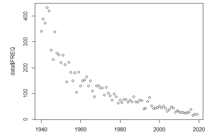
EXERCISE 4.6. (a) We run the following code to plot the counts of lightning deaths against year.
data<- read.csv (file=”./lightningdata.csv”, header=TRUE, sep=”, “)
plot (data\$YEAR, data\$FREQ)
We can see from the plot that the intensity rate decreases over time roughly exponentially. A possible explanation for it is that over the years more awareness has been created among citizens through educational efforts, so fewer people are exposed to the hazard.
(b) We can see that lightning strikes are essentially a seasonal phenomenon. The majority of them happen between May and September. It means that some interarrival times have very large values not inherent to an exponential distribution. Moreover, some incidents resulted in multiple fatalities which would be an event of probability zero under the Poisson law.
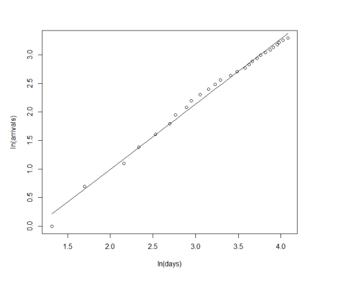
EXERCISE 4.7. (a) The code and output below estimate the parameters of the model using the regression approach.
port. data<- read.csv (file=”./Exercise $4.4$ Data.csv”, header=TRUE, sep=”, “)
$x<-\log$ (port. data\$days)
$y<-\log$ (port. data\$arrivals)
$g \ln \left(y^{\sim} x\right)$
plot $\left(x, y, x l a b=” \ln (\text { days })^{\prime \prime}, \quad y l a b=” \ln (\operatorname{arrivals})^{}\right)$ Coefficients: (Intercept) $\begin{array}{lr}-1.294 & 1.145\end{array}$ $\operatorname{lines}\left(x,-1.294+1.145^{} x\right)$
统计代写|随机过程代写stochastic process代考|The code that follows estimates
(b) The code that follows estimates the parameters using the maximum likelihood approach.
port. data<- read.csv(file=” ./Exercise $4.4$ Data.csv”, header=TRUE, sep=”, “)
$x<-\log$ (port. data\$days)
$y<-\log ($ port. data\$arrivals)
$\mathrm{N}<-27$
print (beta. hat $\left.<-N /\left(N^{*} x[N]-\operatorname{sum}(x)\right)\right)$
- 162782
print (alpha. hat<- N/exp (x[N] *eta . hat) )
$0.2351766$
The MLEs are $\hat{\alpha}=0.2351766$, and $\hat{\beta}=1.162782$.
(c) To predict when the next 10,000 TEUs arrive at the port, we submit the following lines of code.
port. data<- read.csv(file=”. /Exercise4. 4 Data.csv”, header=TRUE, sep=”, “)
$x<-\log ($ port. data\$days)
$y<-\log$ (port.data\$arrivals)
$\mathbb{N}<-27$
alpha. hat<-c(0.274172, 0.2351766)
beta.hat<-c(1.145, 1.162782)
S. hat<- c()
library (pracma)
for $(i$ in $1: 2)$
print (s. hat $[1]<-$ alpha. hat $[i]^{\wedge}(-$
$1 /$ beta.hat [i] $)^{} \exp \left(a 1 p h a \cdot h a t[i]^{} \exp (x[N])^{\wedge} \text { beta.hat }[i]\right)^{}$ gammainc (alpha. hat [i]exp (x[N]) ‘beta.hat [i], 1/beta. hat [i]+1) [2])
$60.85581$ $60.97308$
According to the data, the 27 th arrival was on day $59.1$. The 28 th arrival is predicted to be on day $60.85581$ (by the linear regression), or $60.97308$ (by the maximum likelihood).
统计代写|随机过程代写stochastic process代考|the total amount paid
EXERCISE 5.1. (a) Let $X(t)=\sum_{i=1}^{N(t)} Y_{i}$ be the total amount paid in prizes up to time $t$ hours. We know that it is a compound Poisson process with $N(t) \sim$ Poisson $(1.5 t)$, and $Y_{i}$ independent of each other and $N(t)$. The first two moments of $Y_{1}$ are $E\left(Y_{1}\right)=(\$ 5000)(0.15)+(2000)(0.35)+$ $(\$ 500)(0.2)+(\$ 100)(0.3)=\$ 1,580$, and $E\left(Y_{1}^{2}\right)=(\$ 5000)^{2}(0.15)+(2000)^{2}(0.35)+$ $(\$ 500)^{2}(0.2)+(\$ 100)^{2}(0.3)=\$^{2} 5,203,000 .$
Therefore, the mean of $X(200)$ is $E(X(200))=(1.5)(200)(\$ 1,580)=\$ 474,000$. The variance is $\operatorname{Var}(X(200))=(1.5)(200)\left(\$^{2} 5,203,000\right)=\$^{2} 1,560,900,000$, and the standard deviation is $\sqrt{\operatorname{Var}(X(200))}=\sqrt{\$^{2} 1,560,900,000}=\$ 39,508.23 .$
The budget for 100 games should be $E(X(200))+\sqrt{\operatorname{Var}(X(200))}=\$ 474,000+\$ 39,508.23=$ $\$ 513,508.23$.
(b) Below are the codes, all relevant output, and the graph for the simulated 100 games.
specifying parameters
lambda<- $1.5$
total. hours<- 200
$p<-c(0.15,0.35,0.2,0.3)$
specifying seed set. seed ( 704661$)$ #generating number of prizes nprizes<- rpois (1, lambda*total. hours)
defining vectors
payof $f<-c$ time<- c()
$u<-c()$
setting initial values
specifying se set.seed (704 661 ) #generating numbinising vect nprizes<- rpois #defining vayf<- c() payofime<- c() u<- c() #setting initia) payoff [1]<- 0 u[1]<- 0
generating standard uniforms for (i in 2: (nprizest1))
$u[i]<-$ runif $(1)$
payoff $[i]<-$ payoff [i-1] $+$ amount [sample $(1: 4,1$, prob=p)]
)
computing event times
hour<- total. hours * sort (u)
simulating trajectory
plot (hour, payoff, type=” $1^{\prime \prime}, 1$ ty=1, lwd=2, col=”green”, $x l a b=”$ Hours”, ylab=”Amount
of payoff (\$)”, panel.first = grid())
随机过程代写
统计代写|随机过程代写stochastic process代考|plot the counts of lightning deaths
练习 4.6。(a) 我们运行以下代码来绘制闪电死亡人数与年份的关系图。
数据<- read.csv (file=”./lightningdata.csv”, header=TRUE, sep=”, “)
图(数据$ YEAR,数据$ FREQ)
我们可以从图中看到,强度率随时间大致呈指数下降。对此的一种可能解释是,多年来,通过教育努力提高了公民的意识,因此接触危险的人越来越少。
(b) 我们可以看到,雷击本质上是一种季节性现象。其中大多数发生在 5 月至 9 月之间。这意味着某些到达间隔时间具有非常大的值,而不是指数分布所固有的。此外,一些事件导致多人死亡,根据泊松定律,这将是概率为零的事件。
练习 4.7。(a) 下面的代码和输出使用回归方法估计模型的参数。
港口。数据<- read.csv (file=”./Exercise4.4数据.csv”, header=TRUE, sep=”, “)
X<−日志(端口。数据$天)
是<−日志(港口。数据$抵港)
Gln(是∼X)
阴谋(X,是,Xl一种b=”ln( 天 )′′,是l一种b=”ln(到达))系数:(截距)−1.2941.145 线条(X,−1.294+1.145X)
统计代写|随机过程代写stochastic process代考|The code that follows estimates
(b) 下面的代码使用最大似然法估计参数。
港口。数据<- read.csv(file=” ./Exercise4.4数据.csv”, header=TRUE, sep=”, “)
X<−日志(端口。数据$天)
是<−日志(港口。数据$到达)
ñ<−27
打印(测试版。帽子<−ñ/(ñ∗X[ñ]−和(X)))
- 162782
打印 (alpha. hat<- N/exp (x[N] *eta . hat) )
0.2351766
MLE 是一种^=0.2351766, 和b^=1.162782.
(c) 为了预测下一个 10,000 TEU 何时到达港口,我们提交以下代码行。
港口。数据<- read.csv(file=”./Exercise4.4 Data.csv”, header=TRUE, sep=”, “)
X<−日志(港口。数据$天)
是<−日志(port.data $到达)
ñ<−27
α。hat<-c(0.274172, 0.2351766)
beta.hat<-c(1.145, 1.162782)
S. hat<- c()
库 (pracma)
用于(一世在1:2)
打印 (s. 帽子[1]<−α。帽子[一世]∧(−
1/beta.hat [我])经验(一种1pH一种⋅H一种吨[一世]经验(X[ñ])∧ beta.hat [一世])gammainc (alpha. hat [i]exp (x[N]) ‘beta.hat [i], 1/beta. hat [i]+1) [2])
60.85581 60.97308
据资料显示,27日到达当天59.1. 预计28号当天到货60.85581(通过线性回归),或60.97308(通过最大可能性)。
统计代写|随机过程代写stochastic process代考|the total amount paid
练习 5.1。(a) 让X(吨)=∑一世=1ñ(吨)是一世是截至时间支付的奖金总额吨小时。我们知道这是一个复合泊松过程ñ(吨)∼泊松(1.5吨), 和是一世彼此独立并且ñ(吨). 前两个时刻是1是和(是1)=($5000)(0.15)+(2000)(0.35)+ ($500)(0.2)+($100)(0.3)=$1,580, 和和(是12)=($5000)2(0.15)+(2000)2(0.35)+ ($500)2(0.2)+($100)2(0.3)=$25,203,000.
因此,平均值X(200)是和(X(200))=(1.5)(200)($1,580)=$474,000. 方差为曾是(X(200))=(1.5)(200)($25,203,000)=$21,560,900,000,标准差为曾是(X(200))=$21,560,900,000=$39,508.23.
100场比赛的预算应该是和(X(200))+曾是(X(200))=$474,000+$39,508.23= $513,508.23.
(b) 以下是模拟 100 场比赛的代码、所有相关输出和图表。
指定参数
λ<-1.5
全部的。小时<- 200
p<−C(0.15,0.35,0.2,0.3)
指定种子集。种子 ( 704661)#生成奖品数量 nprizes<- rpois (1, lambda*total. hours)
定义向量
支付F<−C时间<- c()
在<−C()
设置初始值
指定 se set.seed (704 661 ) #generating numbinising vect nprizes<- rpois #defining vayf<- c() payofime<- c() u<- c() #setting initia) payoff [1]<- 0 u[ 1]<- 0
为 (i in 2: (nprizest1)) 生成标准制服
在[一世]<−鲁尼夫(1)
清偿[一世]<−回报 [i-1]+数量 [样品(1:4,1, 概率=p)]
)
计算事件时间
小时<-总计。小时 * 排序 (u)
模拟轨迹
情节(小时,收益,类型=”1′′,1ty=1,lwd=2,col=“绿色”,Xl一种b=”小时”, ylab=”
支付金额 ( $ )”, panel.first = grid())

统计代写请认准statistics-lab™. statistics-lab™为您的留学生涯保驾护航。
金融工程代写
金融工程是使用数学技术来解决金融问题。金融工程使用计算机科学、统计学、经济学和应用数学领域的工具和知识来解决当前的金融问题,以及设计新的和创新的金融产品。
非参数统计代写
非参数统计指的是一种统计方法,其中不假设数据来自于由少数参数决定的规定模型;这种模型的例子包括正态分布模型和线性回归模型。
广义线性模型代考
广义线性模型(GLM)归属统计学领域,是一种应用灵活的线性回归模型。该模型允许因变量的偏差分布有除了正态分布之外的其它分布。
术语 广义线性模型(GLM)通常是指给定连续和/或分类预测因素的连续响应变量的常规线性回归模型。它包括多元线性回归,以及方差分析和方差分析(仅含固定效应)。
有限元方法代写
有限元方法(FEM)是一种流行的方法,用于数值解决工程和数学建模中出现的微分方程。典型的问题领域包括结构分析、传热、流体流动、质量运输和电磁势等传统领域。
有限元是一种通用的数值方法,用于解决两个或三个空间变量的偏微分方程(即一些边界值问题)。为了解决一个问题,有限元将一个大系统细分为更小、更简单的部分,称为有限元。这是通过在空间维度上的特定空间离散化来实现的,它是通过构建对象的网格来实现的:用于求解的数值域,它有有限数量的点。边界值问题的有限元方法表述最终导致一个代数方程组。该方法在域上对未知函数进行逼近。[1] 然后将模拟这些有限元的简单方程组合成一个更大的方程系统,以模拟整个问题。然后,有限元通过变化微积分使相关的误差函数最小化来逼近一个解决方案。
tatistics-lab作为专业的留学生服务机构,多年来已为美国、英国、加拿大、澳洲等留学热门地的学生提供专业的学术服务,包括但不限于Essay代写,Assignment代写,Dissertation代写,Report代写,小组作业代写,Proposal代写,Paper代写,Presentation代写,计算机作业代写,论文修改和润色,网课代做,exam代考等等。写作范围涵盖高中,本科,研究生等海外留学全阶段,辐射金融,经济学,会计学,审计学,管理学等全球99%专业科目。写作团队既有专业英语母语作者,也有海外名校硕博留学生,每位写作老师都拥有过硬的语言能力,专业的学科背景和学术写作经验。我们承诺100%原创,100%专业,100%准时,100%满意。
随机分析代写
随机微积分是数学的一个分支,对随机过程进行操作。它允许为随机过程的积分定义一个关于随机过程的一致的积分理论。这个领域是由日本数学家伊藤清在第二次世界大战期间创建并开始的。
时间序列分析代写
随机过程,是依赖于参数的一组随机变量的全体,参数通常是时间。 随机变量是随机现象的数量表现,其时间序列是一组按照时间发生先后顺序进行排列的数据点序列。通常一组时间序列的时间间隔为一恒定值(如1秒,5分钟,12小时,7天,1年),因此时间序列可以作为离散时间数据进行分析处理。研究时间序列数据的意义在于现实中,往往需要研究某个事物其随时间发展变化的规律。这就需要通过研究该事物过去发展的历史记录,以得到其自身发展的规律。
回归分析代写
多元回归分析渐进(Multiple Regression Analysis Asymptotics)属于计量经济学领域,主要是一种数学上的统计分析方法,可以分析复杂情况下各影响因素的数学关系,在自然科学、社会和经济学等多个领域内应用广泛。
MATLAB代写
MATLAB 是一种用于技术计算的高性能语言。它将计算、可视化和编程集成在一个易于使用的环境中,其中问题和解决方案以熟悉的数学符号表示。典型用途包括:数学和计算算法开发建模、仿真和原型制作数据分析、探索和可视化科学和工程图形应用程序开发,包括图形用户界面构建MATLAB 是一个交互式系统,其基本数据元素是一个不需要维度的数组。这使您可以解决许多技术计算问题,尤其是那些具有矩阵和向量公式的问题,而只需用 C 或 Fortran 等标量非交互式语言编写程序所需的时间的一小部分。MATLAB 名称代表矩阵实验室。MATLAB 最初的编写目的是提供对由 LINPACK 和 EISPACK 项目开发的矩阵软件的轻松访问,这两个项目共同代表了矩阵计算软件的最新技术。MATLAB 经过多年的发展,得到了许多用户的投入。在大学环境中,它是数学、工程和科学入门和高级课程的标准教学工具。在工业领域,MATLAB 是高效研究、开发和分析的首选工具。MATLAB 具有一系列称为工具箱的特定于应用程序的解决方案。对于大多数 MATLAB 用户来说非常重要,工具箱允许您学习和应用专业技术。工具箱是 MATLAB 函数(M 文件)的综合集合,可扩展 MATLAB 环境以解决特定类别的问题。可用工具箱的领域包括信号处理、控制系统、神经网络、模糊逻辑、小波、仿真等。