标签: STAT433

统计代写|随机过程代写stochastic process代考|IE2084

如果你也在 怎样代写随机过程Stochastic Porcesses 这个学科遇到相关的难题,请随时右上角联系我们的24/7代写客服。随机过程Stochastic Porcesses是指一个系统在特定的时间有观测值,结果,即每次的观测值是一个随机变量。

随机过程Stochastic Porcesses在是由一些数学集合索引的随机变量的集合。每个概率和随机过程都与集合中的一个元素唯一地相关联。索引集是用来索引随机变量的集合。索引集传统上是实数的子集,例如自然数,这为索引集提供了时间解释。

statistics-lab™ 为您的留学生涯保驾护航 在代写随机过程stochastic process方面已经树立了自己的口碑, 保证靠谱, 高质且原创的统计Statistics代写服务。我们的专家在代写随机过程stochastic process代写方面经验极为丰富,各种代写随机过程stochastic process相关的作业也就用不着说。

统计代写|随机过程代写stochastic process代考|STAT433

统计代写|随机过程代写stochastic process代考|Probability distribution

It may be seen that the probability distribution of $X_r, X_{r+1}, \ldots, X_{r+n}$ can be computed in terms of the transition probabilities $p_{j k}$ and the initial distribution of $X_r$. Suppose, for simplicity, that $r=0$, then
$$
\begin{aligned}
\operatorname{Pr}\left{X_0\right. & \left.=a, X_1=b, \ldots, X_{n-2}=i, X_{n-1}=j, X_n=k\right} \
& =\operatorname{Pr}\left{X_n=k \mid X_{n-1}=j, \cdots, X_0=a\right} \operatorname{Pr}\left{X_{n-1}=j, \cdots, X_0=a\right} \
& =\operatorname{Pr}\left{X_n=k \mid X_{n-1}=j\right} \operatorname{Pr}\left{X_{n-1}=j \mid X_{n-2}=i\right} \operatorname{Pr}\left{X_{n-2}=i, \cdots, X_0=a\right} \
& =\operatorname{Pr}\left{X_n=k \mid X_{n-1}=j\right} \operatorname{Pr}\left{X_{n-1}=j \mid X_{n-2}=i\right} \cdots \operatorname{Pr}\left{X_1=b \mid X_0=a\right} \operatorname{Pr}\left{X_0=a\right} \
& =\left{\operatorname{Pr}\left(X_0=a\right)\right} p_{a b} \cdots p_{i j} p_{j k} .
\end{aligned}
$$
Thus,
$$
\begin{aligned}
\operatorname{Pr}\left{X_r\right. & \left.=a, X_{r+1}=b, \ldots, X_{r+n-2}=i, X_{r+n-1}=j, X_{r+n}=k\right} \
& =\left{\operatorname{Pr}\left(X_r=a\right)\right} p_{a b} \ldots p_{i j} p_{j k} .
\end{aligned}
$$
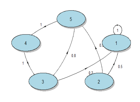
Example 1(g). Let $\left{X_n, n \geq 0\right}$ be a Markov chain with three states $0,1,2$ and with transition matrix
$$
\left(\begin{array}{ccc}
3 / 4 & 1 / 4 & 0 \
1 / 4 & 1 / 2 & 1 / 4 \
0 & 3 / 4 & 1 / 4
\end{array}\right)
$$
and the initial distribution $\operatorname{Pr}\left{X_0=i\right}=\frac{1}{3}, i=0,1,2$.
We have
$$
\begin{aligned}
& \operatorname{Pr}\left{X_1=1 \mid X_0=2\right}=\frac{3}{4} \
& \operatorname{Pr}\left{X_2=2 \mid X_1=1\right}=\frac{1}{4} \
& \operatorname{Pr}\left{X_2=2, X_1=1 \mid X_0=2\right} \
& =\operatorname{Pr}\left{X_2=2 \mid X_1=1\right} \operatorname{Pr}\left{X_1=1 \mid X_0=2\right}=\frac{1}{4} \cdot \frac{3}{4}=\frac{3}{16}
\end{aligned}
$$

\begin{aligned}
\operatorname{Pr}\left{X_2\right. & \left.=2, X_1=1, X_0=2\right} \
& =\operatorname{Pr}\left{X_2=2, X_1=1 \mid X_0=2\right} \operatorname{Pr}\left{X_0=2\right}=\frac{3}{16} \cdot \frac{1}{3}=\frac{1}{16} \
\operatorname{Pr}\left{X_3\right. & \left.=1, X_2=2, X_1=1, X_0=2\right} \
& =\operatorname{Pr}\left{X_3=1 \mid X_2=2, X_1=1, X_0=2\right} \times \operatorname{Pr}\left{X_2=2, X_1=1, X_0=2\right} \
& =\operatorname{Pr}\left{X_3=1 \mid X_2=2\right}\left(\frac{1}{16}\right)=\frac{3}{4} \cdot \frac{1}{16}=\frac{3}{64} .
\end{aligned}

统计代写|随机过程代写stochastic process代考|Strong Markov property

Stopping time for a sequence of r.v.’s $\left{X_n\right}$ is a random variable (see Sec. 6.4.1).
Let $N$ be a stopping time for a Markov chain $\left{X_n, n>0\right}$ and let $A$ and $B$ to two events (relating to $X_n$ and happening) prior and posterior respectively to $N$. Then
$$
\operatorname{Pr}\left{B \mid X_N=i, A\right}=\operatorname{Pr}\left{B \mid X_N=i\right} .
$$
This is called the strong Markov property. It shows that if $N$ is a stopping time for a Markov chain $\left{X_n, n>0\right}$, then the evolution of the chain starts afresh from the state reached at time $N$.

Strong Markov property is implied by the Markov property; both the properties are equivalent when $N$ is constant (a degenerate r.v.).
Every discrete time Markov chain $\left{X_n, n \geq 0\right}$ possesses the strong Markov property.

Definition. A Markov chain $\left{X_n\right}$ is said to be of order $s(s=1,2,3, \ldots)$, if, for all $n$,
$$
\begin{aligned}
\operatorname{Pr}\left{X_n\right. & \left.=k \mid X_{n-1}=j, X_{n-2}=j_1, \ldots, X_{n-s}=j_{s-1}, \ldots\right} \
& =\operatorname{Pr}\left{X_n=k \mid X_{n-1}=j, \ldots, X_{n-s}=j_{s-1}\right} .
\end{aligned}
$$
whenever the 1.h.s. is defined.
A Markov chain $\left{X_n\right}$ is said to be of order one (or simply a Markov chain) if
$$
\begin{aligned}
\operatorname{Pr}\left{X_n\right. & \left.=k \mid X_{n-1}=j, X_{n-2}=j_1, \ldots\right}=\operatorname{Pr}\left{X_n=k \mid X_{n-1}=j\right} \
& =p_{j k} .
\end{aligned}
$$
whenever $\operatorname{Pr}\left{X_{n-1}=j, X_{n-2}=j_1, \ldots\right}>0$.
Unless explicitly stated otherwise, we shall mean by Markov chain, a chain of order one, to which we shall mostly confine ourselves here. A chain is said to be of order zero if $p_{j k}=p_k$ for all $j$. This implies independence of $X_n$ and $X_{n-1}$. For example, for the Bernoulli coin tossing experiment, the t.p.m. is $\left(\begin{array}{ll}q & p \ q & p\end{array}\right)=\left(\begin{array}{l}1 \ 1\end{array}\right)(q, p)=\mathbf{e}(q, p)$.
Denote the state that a day is rainy by 1 and that a day is not rainy by 0 .
Let (1.5) hold for $s=2$ and let
$p_{i j k}=\operatorname{Pr}{$ actual day is in state $k \mid$ the preceding day was in state $j$, the day before the preceding was in state $i}, i, j, k=0,1$.
We then have a Markov chain of order two. Note that the matrix $\left(p_{i j k}\right)$ is not a stochastic matrix. It is a $(4 \times 2)$ matrix and not a square matrix.
Let (1.5) hold for $s=1$ and let
$p_{j k}=\operatorname{Pr}{$ actual day is in state $k \mid$ preceding day was in state $j}$. We then have a Markov chain (i.e. a chain of order one) with t.p.m. $\left(p_{j k}\right), j, k=0,1$.

统计代写|随机过程代写stochastic process代考|STAT433

随机过程代考

统计代写|随机过程代写stochastic process代考|Probability distribution

可以看出,$X_r, X_{r+1}, \ldots, X_{r+n}$的概率分布可以用过渡概率$p_{j k}$和$X_r$的初始分布来计算。为简单起见,假设是$r=0$
$$
\begin{aligned}
\operatorname{Pr}\left{X_0\right. & \left.=a, X_1=b, \ldots, X_{n-2}=i, X_{n-1}=j, X_n=k\right} \
& =\operatorname{Pr}\left{X_n=k \mid X_{n-1}=j, \cdots, X_0=a\right} \operatorname{Pr}\left{X_{n-1}=j, \cdots, X_0=a\right} \
& =\operatorname{Pr}\left{X_n=k \mid X_{n-1}=j\right} \operatorname{Pr}\left{X_{n-1}=j \mid X_{n-2}=i\right} \operatorname{Pr}\left{X_{n-2}=i, \cdots, X_0=a\right} \
& =\operatorname{Pr}\left{X_n=k \mid X_{n-1}=j\right} \operatorname{Pr}\left{X_{n-1}=j \mid X_{n-2}=i\right} \cdots \operatorname{Pr}\left{X_1=b \mid X_0=a\right} \operatorname{Pr}\left{X_0=a\right} \
& =\left{\operatorname{Pr}\left(X_0=a\right)\right} p_{a b} \cdots p_{i j} p_{j k} .
\end{aligned}
$$
因此,
$$
\begin{aligned}
\operatorname{Pr}\left{X_r\right. & \left.=a, X_{r+1}=b, \ldots, X_{r+n-2}=i, X_{r+n-1}=j, X_{r+n}=k\right} \
& =\left{\operatorname{Pr}\left(X_r=a\right)\right} p_{a b} \ldots p_{i j} p_{j k} .
\end{aligned}
$$
例1(g)。设$\left{X_n, n \geq 0\right}$为具有三态$0,1,2$和转移矩阵的马尔可夫链
$$
\left(\begin{array}{ccc}
3 / 4 & 1 / 4 & 0 \
1 / 4 & 1 / 2 & 1 / 4 \
0 & 3 / 4 & 1 / 4
\end{array}\right)
$$
初始分布$\operatorname{Pr}\left{X_0=i\right}=\frac{1}{3}, i=0,1,2$。
我们有
$$
\begin{aligned}
& \operatorname{Pr}\left{X_1=1 \mid X_0=2\right}=\frac{3}{4} \
& \operatorname{Pr}\left{X_2=2 \mid X_1=1\right}=\frac{1}{4} \
& \operatorname{Pr}\left{X_2=2, X_1=1 \mid X_0=2\right} \
& =\operatorname{Pr}\left{X_2=2 \mid X_1=1\right} \operatorname{Pr}\left{X_1=1 \mid X_0=2\right}=\frac{1}{4} \cdot \frac{3}{4}=\frac{3}{16}
\end{aligned}
$$

\begin{aligned}
\operatorname{Pr}\left{X_2\right. & \left.=2, X_1=1, X_0=2\right} \& =\operatorname{Pr}\left{X_2=2, X_1=1 \mid X_0=2\right} \operatorname{Pr}\left{X_0=2\right}=\frac{3}{16} \cdot \frac{1}{3}=\frac{1}{16} \operatorname{Pr}\left{X_3\right. & \left.=1, X_2=2, X_1=1, X_0=2\right} \& =\operatorname{Pr}\left{X_3=1 \mid X_2=2, X_1=1, X_0=2\right} \times \operatorname{Pr}\left{X_2=2, X_1=1, X_0=2\right} \& =\operatorname{Pr}\left{X_3=1 \mid X_2=2\right}\left(\frac{1}{16}\right)=\frac{3}{4} \cdot \frac{1}{16}=\frac{3}{64} .
\end{aligned}

统计代写|随机过程代写stochastic process代考|Strong Markov property

rv序列的停止时间。的$\left{X_n\right}$是一个随机变量(见第6.4.1节)。
设$N$为马尔可夫链$\left{X_n, n>0\right}$的停止时间,并设$A$和$B$分别表示两个事件(与$X_n$和正在发生的事件有关)在$N$之前和之后。然后
$$
\operatorname{Pr}\left{B \mid X_N=i, A\right}=\operatorname{Pr}\left{B \mid X_N=i\right} .
$$
这被称为强马尔可夫性质。它表明,如果$N$是马尔可夫链$\left{X_n, n>0\right}$的停止时间,则该链的进化从时间$N$所达到的状态重新开始。

强马尔可夫性质由马尔可夫性质隐含;当$N$为常数时,这两个属性是等价的(简并的r.v.)。
每一个离散时间马尔可夫链$\left{X_n, n \geq 0\right}$都具有强马尔可夫性。

定义。一个马尔可夫链$\left{X_n\right}$的阶为$s(s=1,2,3, \ldots)$,如果对于所有$n$,
$$
\begin{aligned}
\operatorname{Pr}\left{X_n\right. & \left.=k \mid X_{n-1}=j, X_{n-2}=j_1, \ldots, X_{n-s}=j_{s-1}, \ldots\right} \
& =\operatorname{Pr}\left{X_n=k \mid X_{n-1}=j, \ldots, X_{n-s}=j_{s-1}\right} .
\end{aligned}
$$
每当1。h。s。已定义。
一个马尔可夫链$\left{X_n\right}$被认为是一阶(或简单的马尔可夫链),如果
$$
\begin{aligned}
\operatorname{Pr}\left{X_n\right. & \left.=k \mid X_{n-1}=j, X_{n-2}=j_1, \ldots\right}=\operatorname{Pr}\left{X_n=k \mid X_{n-1}=j\right} \
& =p_{j k} .
\end{aligned}
$$
每当$\operatorname{Pr}\left{X_{n-1}=j, X_{n-2}=j_1, \ldots\right}>0$。
除非另有明确说明,我们所说的马尔可夫链是指一阶的链,我们在这里主要限于此。如果$p_{j k}=p_k$对于所有的$j$链都是0阶。这意味着$X_n$和$X_{n-1}$的独立性。例如,在伯努利抛硬币实验中,t.p.m.是$\left(\begin{array}{ll}q & p \ q & p\end{array}\right)=\left(\begin{array}{l}1 \ 1\end{array}\right)(q, p)=\mathbf{e}(q, p)$。
表示某天下雨的状态为1,某天不下雨的状态为0。
Let (1.5) hold for $s=2$, Let
$p_{i j k}=\operatorname{Pr}{$实际日期为状态$k \mid$前一天为状态$j$,前一天为状态$i}, i, j, k=0,1$。
然后我们有一个二阶马尔可夫链。注意,矩阵$\left(p_{i j k}\right)$不是一个随机矩阵。它是一个$(4 \times 2)$矩阵而不是一个方阵。
Let (1.5) hold for $s=1$, Let
$p_{j k}=\operatorname{Pr}{$实际日期为$k \mid$前一天为$j}$。然后我们有一个带有t.p.m. $\left(p_{j k}\right), j, k=0,1$的马尔可夫链(即一阶链)。

数学代写|随机过程统计代写Stochastic process statistics代考 请认准statistics-lab™

统计代写请认准statistics-lab™. statistics-lab™为您的留学生涯保驾护航。

金融工程代写

金融工程是使用数学技术来解决金融问题。金融工程使用计算机科学、统计学、经济学和应用数学领域的工具和知识来解决当前的金融问题,以及设计新的和创新的金融产品。

非参数统计代写

非参数统计指的是一种统计方法,其中不假设数据来自于由少数参数决定的规定模型;这种模型的例子包括正态分布模型和线性回归模型。

广义线性模型代考

广义线性模型(GLM)归属统计学领域,是一种应用灵活的线性回归模型。该模型允许因变量的偏差分布有除了正态分布之外的其它分布。

术语 广义线性模型(GLM)通常是指给定连续和/或分类预测因素的连续响应变量的常规线性回归模型。它包括多元线性回归,以及方差分析和方差分析(仅含固定效应)。

有限元方法代写

有限元方法(FEM)是一种流行的方法,用于数值解决工程和数学建模中出现的微分方程。典型的问题领域包括结构分析、传热、流体流动、质量运输和电磁势等传统领域。

有限元是一种通用的数值方法,用于解决两个或三个空间变量的偏微分方程(即一些边界值问题)。为了解决一个问题,有限元将一个大系统细分为更小、更简单的部分,称为有限元。这是通过在空间维度上的特定空间离散化来实现的,它是通过构建对象的网格来实现的:用于求解的数值域,它有有限数量的点。边界值问题的有限元方法表述最终导致一个代数方程组。该方法在域上对未知函数进行逼近。[1] 然后将模拟这些有限元的简单方程组合成一个更大的方程系统,以模拟整个问题。然后,有限元通过变化微积分使相关的误差函数最小化来逼近一个解决方案。

tatistics-lab作为专业的留学生服务机构,多年来已为美国、英国、加拿大、澳洲等留学热门地的学生提供专业的学术服务,包括但不限于Essay代写,Assignment代写,Dissertation代写,Report代写,小组作业代写,Proposal代写,Paper代写,Presentation代写,计算机作业代写,论文修改和润色,网课代做,exam代考等等。写作范围涵盖高中,本科,研究生等海外留学全阶段,辐射金融,经济学,会计学,审计学,管理学等全球99%专业科目。写作团队既有专业英语母语作者,也有海外名校硕博留学生,每位写作老师都拥有过硬的语言能力,专业的学科背景和学术写作经验。我们承诺100%原创,100%专业,100%准时,100%满意。

随机分析代写


随机微积分是数学的一个分支,对随机过程进行操作。它允许为随机过程的积分定义一个关于随机过程的一致的积分理论。这个领域是由日本数学家伊藤清在第二次世界大战期间创建并开始的。

时间序列分析代写

随机过程,是依赖于参数的一组随机变量的全体,参数通常是时间。 随机变量是随机现象的数量表现,其时间序列是一组按照时间发生先后顺序进行排列的数据点序列。通常一组时间序列的时间间隔为一恒定值(如1秒,5分钟,12小时,7天,1年),因此时间序列可以作为离散时间数据进行分析处理。研究时间序列数据的意义在于现实中,往往需要研究某个事物其随时间发展变化的规律。这就需要通过研究该事物过去发展的历史记录,以得到其自身发展的规律。

回归分析代写

多元回归分析渐进(Multiple Regression Analysis Asymptotics)属于计量经济学领域,主要是一种数学上的统计分析方法,可以分析复杂情况下各影响因素的数学关系,在自然科学、社会和经济学等多个领域内应用广泛。

MATLAB代写

MATLAB 是一种用于技术计算的高性能语言。它将计算、可视化和编程集成在一个易于使用的环境中,其中问题和解决方案以熟悉的数学符号表示。典型用途包括:数学和计算算法开发建模、仿真和原型制作数据分析、探索和可视化科学和工程图形应用程序开发,包括图形用户界面构建MATLAB 是一个交互式系统,其基本数据元素是一个不需要维度的数组。这使您可以解决许多技术计算问题,尤其是那些具有矩阵和向量公式的问题,而只需用 C 或 Fortran 等标量非交互式语言编写程序所需的时间的一小部分。MATLAB 名称代表矩阵实验室。MATLAB 最初的编写目的是提供对由 LINPACK 和 EISPACK 项目开发的矩阵软件的轻松访问,这两个项目共同代表了矩阵计算软件的最新技术。MATLAB 经过多年的发展,得到了许多用户的投入。在大学环境中,它是数学、工程和科学入门和高级课程的标准教学工具。在工业领域,MATLAB 是高效研究、开发和分析的首选工具。MATLAB 具有一系列称为工具箱的特定于应用程序的解决方案。对于大多数 MATLAB 用户来说非常重要,工具箱允许您学习应用专业技术。工具箱是 MATLAB 函数(M 文件)的综合集合,可扩展 MATLAB 环境以解决特定类别的问题。可用工具箱的领域包括信号处理、控制系统、神经网络、模糊逻辑、小波、仿真等。

R语言代写问卷设计与分析代写
PYTHON代写回归分析与线性模型代写
MATLAB代写方差分析与试验设计代写
STATA代写机器学习/统计学习代写
SPSS代写计量经济学代写
EVIEWS代写时间序列分析代写
EXCEL代写深度学习代写
SQL代写各种数据建模与可视化代写

统计代写|随机过程代写stochastic process代考|STAT433

如果你也在 怎样代写随机过程Stochastic Porcesses 这个学科遇到相关的难题,请随时右上角联系我们的24/7代写客服。随机过程Stochastic Porcesses是指一个系统在特定的时间有观测值,结果,即每次的观测值是一个随机变量。

随机过程Stochastic Porcesses在是由一些数学集合索引的随机变量的集合。每个概率和随机过程都与集合中的一个元素唯一地相关联。索引集是用来索引随机变量的集合。索引集传统上是实数的子集,例如自然数,这为索引集提供了时间解释。

statistics-lab™ 为您的留学生涯保驾护航 在代写随机过程stochastic process方面已经树立了自己的口碑, 保证靠谱, 高质且原创的统计Statistics代写服务。我们的专家在代写随机过程stochastic process代写方面经验极为丰富,各种代写随机过程stochastic process相关的作业也就用不着说。

统计代写|随机过程代写stochastic process代考|STAT433

统计代写|随机过程代写stochastic process代考|DEFINITION AND EXAMPLES

Consider a simple coin tossing experiment repeated for a number of times. The possible outcomes at each trial are two: head with probability, say, $p$ and tail with probability $q, p+q=1$. Let us denote head by 1 and tail by 0 and the random variable denoting the result of the $n$th toss by $X_n$. Then for $n=1,2$, $3, \ldots$,
$$
\operatorname{Pr}\left(X_n=1\right)=p, \operatorname{Pr}\left{X_n=0\right}=q .
$$
Thus we have a sequence of random variables $X_1, X_2, \ldots$. The trials are independent and the result of the $n$th trial does not depend in any way on the previous trials numbered $1,2, \ldots,(n-1)$. The random variables are independent.

Consider now the random variable given by the partial sum $S_n=X_1+\cdots+X_n$. The sum $S_n$ gives the accumulated number of heads in the first $n$ trials and its possible values are $0,1, \ldots, n$.

We have $S_{n+1}=S_n+X_{n+1}$. Given that $S_n=j(j=0,1, \ldots, n)$, the r.v. $S_{n+1}$ can assume only two possible values: $S_{n+1}=j$ with probability $q$ and $S_{n+1}=j+1$ with probability $p$; these probabilities are not at all affected by the values of the variables $S_1, \ldots, S_{n-1}$. Thus
$$
\begin{aligned}
& \operatorname{Pr}\left{S_{n+1}=j+1 \mid S_n=j\right}=p \
& \operatorname{Pr}\left{S_{n+1}=j \mid S_n=j\right}=q .
\end{aligned}
$$
We have here an example of a Markov* chain, a case of simple dependence that the outcome of $(n+1)$ st trial depends directly on that of $n$th trial and only on it. The conditional probability of $S_{n+1}$ given $S_n$ depends on the value of $S_n$ and the manner in which the value of $S_n$ was reached is of no consequence.

统计代写|随机过程代写stochastic process代考|Transition Matrix (or Matrix of Transition Probabilities)

The transition probabilities $p_{j k}$ satisfy
$$
p_{j k} \geq 0, \quad \sum_k p_{j k}=1 \text { for all } j .
$$
These probabilities may be written in the matrix form
$$
P=\left(\begin{array}{cccc}
p_{11} & p_{12} & p_{13} & \cdots \
p_{21} & p_{22} & p_{23} & \cdots \
\cdots & \cdots & \ldots & \ldots \
\cdots & \ldots & \ldots & \ldots
\end{array}\right)
$$
This is called the transition probability matrix or matrix of transition probabilities (t.p.m.) of the Markov chain. $P$ is a stochastic matrix i.e. a square matrix with non-negative elements and unit row sums.

Example 1(b). A particle performs a random walk with absorbing barriers, say, as 0 and 4 . Whenever it is at any position $r(0<r<4)$, it moves to $r+1$ with probability $P$ or to $(r-1)$ with probability $q$, $p+q=1$. But as soon as it reaches 0 or 4 it remains there itself. Let $X_n$ be the position of the particle after $n$ moves. The different states of $X_n$ are the different positions of the particle. $\left{X_n\right}$ is a Markov chain whose unit-step transition probabilities are given by
$$
\begin{array}{ll}
\operatorname{Pr}\left{X_n=r+1 \mid X_{n-1}=r\right}=p & \
\operatorname{Pr}\left{X_n=r-1 \mid X_{n-1}=r\right}=q & 0<r<4
\end{array}
$$
and
$$
\begin{aligned}
& \operatorname{Pr}\left{X_n=0 \mid X_{n-1}=0\right}=1, \
& \operatorname{Pr}\left{X_n=4 \mid X_{n-1}=4\right}=1 .
\end{aligned}
$$

The transition matrix is given by
$$
\left.\begin{array}{ccccccc}
\text { States of } X_{n-1} & \multicolumn{7}{c}{\text { States of } X_n} \
& & 0 & 1 & 2 & 3 & 4 \
& 1 & & 0 & 0 & 0 & 0 \
& 2 & 0 & p & 0 & 0 \
& 3 \
& 4 & q & 0 & p & 0 \
0 & 0 & q & 0 & p \
0 & 0 & 0 & 0 & 1
\end{array}\right)
$$

统计代写|随机过程代写stochastic process代考|STAT433

随机过程代考

统计代写|随机过程代写stochastic process代考|DEFINITION AND EXAMPLES

考虑一个重复多次的简单抛硬币实验。每次试验都有两种可能的结果:有概率的正面,比如, $p$ 尾部是概率 $q, p+q=1$. 让我们用1表示头,用0表示尾随机变量表示的结果 $n$扔过去 $X_n$. 然后是 $n=1,2$, $3, \ldots$,
$$
\operatorname{Pr}\left(X_n=1\right)=p, \operatorname{Pr}\left{X_n=0\right}=q .
$$
这样我们就得到了一个随机变量序列 $X_1, X_2, \ldots$. 试验是独立的,结果是 $n$该试验不以任何方式依赖于先前试验的编号 $1,2, \ldots,(n-1)$. 随机变量是独立的。

现在考虑部分和$S_n=X_1+\cdots+X_n$给出的随机变量。和$S_n$给出了在第一次$n$次试验中累积的正面数,它的可能值是$0,1, \ldots, n$。

我们有$S_{n+1}=S_n+X_{n+1}$。给定$S_n=j(j=0,1, \ldots, n)$, rv $S_{n+1}$只能假设两个可能的值:$S_{n+1}=j$的概率为$q$, $S_{n+1}=j+1$的概率为$p$;这些概率完全不受$S_1, \ldots, S_{n-1}$变量值的影响。因此
$$
\begin{aligned}
& \operatorname{Pr}\left{S_{n+1}=j+1 \mid S_n=j\right}=p \
& \operatorname{Pr}\left{S_{n+1}=j \mid S_n=j\right}=q .
\end{aligned}
$$
我们这里有一个马尔可夫链的例子,这是一个简单依赖的例子,即$(n+1)$第一次试验的结果直接依赖于$n$第二次试验的结果,而且只依赖于它。给定$S_n$的$S_{n+1}$的条件概率取决于$S_n$的值,而达到$S_n$值的方式无关紧要。

统计代写|随机过程代写stochastic process代考|Transition Matrix (or Matrix of Transition Probabilities)

跃迁概率$p_{j k}$满足
$$
p_{j k} \geq 0, \quad \sum_k p_{j k}=1 \text { for all } j .
$$
这些概率可以写成矩阵形式
$$
P=\left(\begin{array}{cccc}
p_{11} & p_{12} & p_{13} & \cdots \
p_{21} & p_{22} & p_{23} & \cdots \
\cdots & \cdots & \ldots & \ldots \
\cdots & \ldots & \ldots & \ldots
\end{array}\right)
$$
这被称为马尔可夫链的转移概率矩阵或转移概率矩阵。$P$是一个随机矩阵,即具有非负元素和单位行和的方阵。

例1(b)。粒子进行随机游走,有吸收障碍,比如0和4。当它在任何位置$r(0<r<4)$时,它以$P$的概率移动到$r+1$,或以$q$, $p+q=1$的概率移动到$(r-1)$。但一旦它达到0或4,它就会保持在那里。设$X_n$为$n$移动后粒子的位置。$X_n$的不同状态是粒子的不同位置。$\left{X_n\right}$是一个马尔可夫链,其单位阶跃转移概率由式给出
$$
\begin{array}{ll}
\operatorname{Pr}\left{X_n=r+1 \mid X_{n-1}=r\right}=p & \
\operatorname{Pr}\left{X_n=r-1 \mid X_{n-1}=r\right}=q & 0<r<4
\end{array}
$$

$$
\begin{aligned}
& \operatorname{Pr}\left{X_n=0 \mid X_{n-1}=0\right}=1, \
& \operatorname{Pr}\left{X_n=4 \mid X_{n-1}=4\right}=1 .
\end{aligned}
$$

转移矩阵由
$$
\left.\begin{array}{ccccccc}
\text { States of } X_{n-1} & \multicolumn{7}{c}{\text { States of } X_n} \
& & 0 & 1 & 2 & 3 & 4 \
& 1 & & 0 & 0 & 0 & 0 \
& 2 & 0 & p & 0 & 0 \
& 3 \
& 4 & q & 0 & p & 0 \
0 & 0 & q & 0 & p \
0 & 0 & 0 & 0 & 1
\end{array}\right)
$$

数学代写|随机过程统计代写Stochastic process statistics代考 请认准statistics-lab™

统计代写请认准statistics-lab™. statistics-lab™为您的留学生涯保驾护航。

金融工程代写

金融工程是使用数学技术来解决金融问题。金融工程使用计算机科学、统计学、经济学和应用数学领域的工具和知识来解决当前的金融问题,以及设计新的和创新的金融产品。

非参数统计代写

非参数统计指的是一种统计方法,其中不假设数据来自于由少数参数决定的规定模型;这种模型的例子包括正态分布模型和线性回归模型。

广义线性模型代考

广义线性模型(GLM)归属统计学领域,是一种应用灵活的线性回归模型。该模型允许因变量的偏差分布有除了正态分布之外的其它分布。

术语 广义线性模型(GLM)通常是指给定连续和/或分类预测因素的连续响应变量的常规线性回归模型。它包括多元线性回归,以及方差分析和方差分析(仅含固定效应)。

有限元方法代写

有限元方法(FEM)是一种流行的方法,用于数值解决工程和数学建模中出现的微分方程。典型的问题领域包括结构分析、传热、流体流动、质量运输和电磁势等传统领域。

有限元是一种通用的数值方法,用于解决两个或三个空间变量的偏微分方程(即一些边界值问题)。为了解决一个问题,有限元将一个大系统细分为更小、更简单的部分,称为有限元。这是通过在空间维度上的特定空间离散化来实现的,它是通过构建对象的网格来实现的:用于求解的数值域,它有有限数量的点。边界值问题的有限元方法表述最终导致一个代数方程组。该方法在域上对未知函数进行逼近。[1] 然后将模拟这些有限元的简单方程组合成一个更大的方程系统,以模拟整个问题。然后,有限元通过变化微积分使相关的误差函数最小化来逼近一个解决方案。

tatistics-lab作为专业的留学生服务机构,多年来已为美国、英国、加拿大、澳洲等留学热门地的学生提供专业的学术服务,包括但不限于Essay代写,Assignment代写,Dissertation代写,Report代写,小组作业代写,Proposal代写,Paper代写,Presentation代写,计算机作业代写,论文修改和润色,网课代做,exam代考等等。写作范围涵盖高中,本科,研究生等海外留学全阶段,辐射金融,经济学,会计学,审计学,管理学等全球99%专业科目。写作团队既有专业英语母语作者,也有海外名校硕博留学生,每位写作老师都拥有过硬的语言能力,专业的学科背景和学术写作经验。我们承诺100%原创,100%专业,100%准时,100%满意。

随机分析代写


随机微积分是数学的一个分支,对随机过程进行操作。它允许为随机过程的积分定义一个关于随机过程的一致的积分理论。这个领域是由日本数学家伊藤清在第二次世界大战期间创建并开始的。

时间序列分析代写

随机过程,是依赖于参数的一组随机变量的全体,参数通常是时间。 随机变量是随机现象的数量表现,其时间序列是一组按照时间发生先后顺序进行排列的数据点序列。通常一组时间序列的时间间隔为一恒定值(如1秒,5分钟,12小时,7天,1年),因此时间序列可以作为离散时间数据进行分析处理。研究时间序列数据的意义在于现实中,往往需要研究某个事物其随时间发展变化的规律。这就需要通过研究该事物过去发展的历史记录,以得到其自身发展的规律。

回归分析代写

多元回归分析渐进(Multiple Regression Analysis Asymptotics)属于计量经济学领域,主要是一种数学上的统计分析方法,可以分析复杂情况下各影响因素的数学关系,在自然科学、社会和经济学等多个领域内应用广泛。

MATLAB代写

MATLAB 是一种用于技术计算的高性能语言。它将计算、可视化和编程集成在一个易于使用的环境中,其中问题和解决方案以熟悉的数学符号表示。典型用途包括:数学和计算算法开发建模、仿真和原型制作数据分析、探索和可视化科学和工程图形应用程序开发,包括图形用户界面构建MATLAB 是一个交互式系统,其基本数据元素是一个不需要维度的数组。这使您可以解决许多技术计算问题,尤其是那些具有矩阵和向量公式的问题,而只需用 C 或 Fortran 等标量非交互式语言编写程序所需的时间的一小部分。MATLAB 名称代表矩阵实验室。MATLAB 最初的编写目的是提供对由 LINPACK 和 EISPACK 项目开发的矩阵软件的轻松访问,这两个项目共同代表了矩阵计算软件的最新技术。MATLAB 经过多年的发展,得到了许多用户的投入。在大学环境中,它是数学、工程和科学入门和高级课程的标准教学工具。在工业领域,MATLAB 是高效研究、开发和分析的首选工具。MATLAB 具有一系列称为工具箱的特定于应用程序的解决方案。对于大多数 MATLAB 用户来说非常重要,工具箱允许您学习应用专业技术。工具箱是 MATLAB 函数(M 文件)的综合集合,可扩展 MATLAB 环境以解决特定类别的问题。可用工具箱的领域包括信号处理、控制系统、神经网络、模糊逻辑、小波、仿真等。

R语言代写问卷设计与分析代写
PYTHON代写回归分析与线性模型代写
MATLAB代写方差分析与试验设计代写
STATA代写机器学习/统计学习代写
SPSS代写计量经济学代写
EVIEWS代写时间序列分析代写
EXCEL代写深度学习代写
SQL代写各种数据建模与可视化代写

统计代写|随机过程代写stochastic process代考|BISSP2023

如果你也在 怎样代写随机过程Stochastic Porcesses 这个学科遇到相关的难题,请随时右上角联系我们的24/7代写客服。随机过程Stochastic Porcesses是指一个系统在特定的时间有观测值,结果,即每次的观测值是一个随机变量。

随机过程Stochastic Porcesses在是由一些数学集合索引的随机变量的集合。每个概率和随机过程都与集合中的一个元素唯一地相关联。索引集是用来索引随机变量的集合。索引集传统上是实数的子集,例如自然数,这为索引集提供了时间解释。

statistics-lab™ 为您的留学生涯保驾护航 在代写随机过程stochastic process方面已经树立了自己的口碑, 保证靠谱, 高质且原创的统计Statistics代写服务。我们的专家在代写随机过程stochastic process代写方面经验极为丰富,各种代写随机过程stochastic process相关的作业也就用不着说。

统计代写|随机过程代写stochastic process代考|BISSP2023

统计代写|随机过程代写stochastic process代考|Specification of Stochastic Processes

The set of possible values of a single random variable $X_n$ of a stochastic process $\left{X_n, n \geq 1\right}$ is known as its state space. The state space is discrete if it contains a finite or a denumerable infinity of points; otherwise, it is continuous. For example, if $X_n$ is the total number of sixes appearing in the first $n$ throws of a die, the set of possible values of $X_n$ is the finite set of non-negative integers $0,1, \ldots, n$. Here, the state space of $X_n$ is discrete. We can write $X_n=Y_1+\cdots+Y_n$, where $Y_i$ is a discrete r.v. denoting the outcome of the $i$ th throw and $Y_i=1$ or 0 according as the $i$ th throw shows six or not. Secondly, consider $X_n=Z_1$ $+\ldots+Z_n$, where $Z_i$ is a continuous r.v. assuming values in $[0, \infty]$. Here, the set of possible values of $X_n$ is the interval $[0, \infty]$, and so the state space of $X_n$ is continuous.

In the above two examples we assume that the parameter $n$ of $X_n$ is restricted to the non-negative integers $n=0,1,2, \ldots$ We consider the state of the system at distinct time points $n=0,1,2, \ldots$, only. Here the word time is used in a wide sense. We note that in the first case considered above the “time $n$ ” implies throw number $n$.

On the other hand, one can visualise a family of random variables $\left{X_v, t \in T\right}$ (or ${X(t), t \in T}$ ) such that the state of the system is characterized at every instant over a finite or infinite interval. The system is then defined for a continuous range of time and we say that we have a family of r.v. in continuous time. A stochastic process in continuous time may have either a discrete or a continuous state space. For example, suppose that $X(t)$ gives the number of incoming calls at a switchboard in an interval $(0, t)$. Here the state space of $X(t)$ is discrete though $X(t)$ is defined for a continuous range of time. We have a process in continuous time having a discrete state space. Suppose that $X(t)$ represents the maximum temperature at a particular place in $(0, t)$, then the set of possible values of $X(t)$ is continuous. Here we have a system in continuous time having a continuous state space.

So far we have assumed that the values assumed by the r.v. $X_n$ (or $\left.X(t)\right)$ are one-dimensional, but the process $\left{X_n\right}$ (or ${X(t)}$ ) may be multi-dimensional. Consider $X(t)=\left(X_1(t), X_2(t)\right.$ ), where $X_1$ represents the maximum and $X_2$ the minimum temperature at a place in an interval of time $(0, t)$. We have here a two-dimensional stochastic process in continuous time having continuous state space. One can similarly have multi-dimensional processes. One-dimensional processes can be classified, in general, into the following four types of processes:
(i) Discrete time, discrete state space
(ii) Discrete time, continuous state space
(iii) Continuous time, discrete state space
(iv) Continuous time, continuous state space.

统计代写|随机过程代写stochastic process代考|Processes with independent increments

If for all $t_1, \ldots, t_n, t_1s$, do not depend on the values of $X(u), u<s$, then the process is said to be a Markov process.
A definition of such a process is given below.
If, for, $t_1<t_2<\ldots<t_n<t$
$$
\begin{aligned}
\operatorname{Pr}\left{a \leq X(t) \leq b \mid X\left(t_1\right)\right. & \left.=x_1, \ldots, X\left(t_n\right)=x_n\right} \
& =\operatorname{Pr}\left{a \leq X(t) \leq b \mid X\left(t_n\right)=x_n\right}
\end{aligned}
$$
the process ${X(t), t \in T}$ is a Markov process.
A discrete parameter Markov process is known as a Markov chain.

统计代写|随机过程代写stochastic process代考|BISSP2023

随机过程代考

统计代写|随机过程代写stochastic process代考|Specification of Stochastic Processes

随机过程$\left{X_n, n \geq 1\right}$的单个随机变量$X_n$的可能值的集合称为其状态空间。如果状态空间包含有限或无限的点,则状态空间是离散的;否则为连续。例如,如果$X_n$是第一次$n$次掷骰子中出现的6的总数,那么$X_n$的可能值的集合就是非负整数$0,1, \ldots, n$的有限集合。这里,$X_n$的状态空间是离散的。我们可以写$X_n=Y_1+\cdots+Y_n$,其中$Y_i$是一个离散的rv,表示$i$次投掷的结果,根据$i$次投掷是否显示6,表示$Y_i=1$或0。其次,考虑$X_n=Z_1$$+\ldots+Z_n$,其中$Z_i$是一个连续的rv,假设$[0, \infty]$中的值。这里,$X_n$的可能值的集合是区间$[0, \infty]$,因此$X_n$的状态空间是连续的。

在上面的两个例子中,我们假设$X_n$的参数$n$被限制为非负整数$n=0,1,2, \ldots$,我们只考虑系统在不同时间点$n=0,1,2, \ldots$的状态。在这里,时间这个词是广义的。我们注意到,在上面考虑的第一种情况中,“时间$n$”意味着抛出数$n$。

另一方面,人们可以想象一组随机变量$\left{X_v, t \in T\right}$(或${X(t), t \in T}$),这样系统的状态在有限或无限区间内的每个瞬间都是有特征的。然后在连续时间范围内定义系统我们说我们有一个连续时间的rv族。连续时间的随机过程可以具有离散状态空间,也可以具有连续状态空间。例如,假设$X(t)$给出了在一个间隔$(0, t)$内总机的入站呼叫数。这里$X(t)$的状态空间是离散的,尽管$X(t)$是在连续时间范围内定义的。我们有一个连续时间的过程有一个离散的状态空间。假设$X(t)$代表$(0, t)$某一特定地点的最高温度,那么$X(t)$的可能值集是连续的。这里我们有一个连续时间系统有一个连续状态空间。

到目前为止,我们已经假定rv $X_n$(或$\left.X(t)\right)$)所假定的值是一维的,但是过程$\left{X_n\right}$(或${X(t)}$)可能是多维的。考虑$X(t)=\left(X_1(t), X_2(t)\right.$),其中$X_1$表示一段时间内某一地点的最高温度,$X_2$表示一段时间内某一地点的最低温度$(0, t)$。我们这里有一个连续时间的二维随机过程具有连续状态空间。一个人也可以有类似的多维过程。一维过程一般可分为以下四类过程:
(i)离散时间,离散状态空间
(ii)离散时间,连续状态空间
(iii)连续时间,离散状态空间
(iv)连续时间,连续状态空间。

统计代写|随机过程代写stochastic process代考|Processes with independent increments

如果对于所有的$t_1, \ldots, t_n, t_1s$,不依赖于$X(u), u<s$的值,那么这个过程就是一个马尔可夫过程。
下面给出了这种过程的定义。
如果,for, $t_1<t_2<\ldots<t_n<t$
$$
\begin{aligned}
\operatorname{Pr}\left{a \leq X(t) \leq b \mid X\left(t_1\right)\right. & \left.=x_1, \ldots, X\left(t_n\right)=x_n\right} \
& =\operatorname{Pr}\left{a \leq X(t) \leq b \mid X\left(t_n\right)=x_n\right}
\end{aligned}
$$
这个过程${X(t), t \in T}$是一个马尔可夫过程。
离散参数马尔可夫过程称为马尔可夫链。

数学代写|随机过程统计代写Stochastic process statistics代考 请认准statistics-lab™

统计代写请认准statistics-lab™. statistics-lab™为您的留学生涯保驾护航。

金融工程代写

金融工程是使用数学技术来解决金融问题。金融工程使用计算机科学、统计学、经济学和应用数学领域的工具和知识来解决当前的金融问题,以及设计新的和创新的金融产品。

非参数统计代写

非参数统计指的是一种统计方法,其中不假设数据来自于由少数参数决定的规定模型;这种模型的例子包括正态分布模型和线性回归模型。

广义线性模型代考

广义线性模型(GLM)归属统计学领域,是一种应用灵活的线性回归模型。该模型允许因变量的偏差分布有除了正态分布之外的其它分布。

术语 广义线性模型(GLM)通常是指给定连续和/或分类预测因素的连续响应变量的常规线性回归模型。它包括多元线性回归,以及方差分析和方差分析(仅含固定效应)。

有限元方法代写

有限元方法(FEM)是一种流行的方法,用于数值解决工程和数学建模中出现的微分方程。典型的问题领域包括结构分析、传热、流体流动、质量运输和电磁势等传统领域。

有限元是一种通用的数值方法,用于解决两个或三个空间变量的偏微分方程(即一些边界值问题)。为了解决一个问题,有限元将一个大系统细分为更小、更简单的部分,称为有限元。这是通过在空间维度上的特定空间离散化来实现的,它是通过构建对象的网格来实现的:用于求解的数值域,它有有限数量的点。边界值问题的有限元方法表述最终导致一个代数方程组。该方法在域上对未知函数进行逼近。[1] 然后将模拟这些有限元的简单方程组合成一个更大的方程系统,以模拟整个问题。然后,有限元通过变化微积分使相关的误差函数最小化来逼近一个解决方案。

tatistics-lab作为专业的留学生服务机构,多年来已为美国、英国、加拿大、澳洲等留学热门地的学生提供专业的学术服务,包括但不限于Essay代写,Assignment代写,Dissertation代写,Report代写,小组作业代写,Proposal代写,Paper代写,Presentation代写,计算机作业代写,论文修改和润色,网课代做,exam代考等等。写作范围涵盖高中,本科,研究生等海外留学全阶段,辐射金融,经济学,会计学,审计学,管理学等全球99%专业科目。写作团队既有专业英语母语作者,也有海外名校硕博留学生,每位写作老师都拥有过硬的语言能力,专业的学科背景和学术写作经验。我们承诺100%原创,100%专业,100%准时,100%满意。

随机分析代写


随机微积分是数学的一个分支,对随机过程进行操作。它允许为随机过程的积分定义一个关于随机过程的一致的积分理论。这个领域是由日本数学家伊藤清在第二次世界大战期间创建并开始的。

时间序列分析代写

随机过程,是依赖于参数的一组随机变量的全体,参数通常是时间。 随机变量是随机现象的数量表现,其时间序列是一组按照时间发生先后顺序进行排列的数据点序列。通常一组时间序列的时间间隔为一恒定值(如1秒,5分钟,12小时,7天,1年),因此时间序列可以作为离散时间数据进行分析处理。研究时间序列数据的意义在于现实中,往往需要研究某个事物其随时间发展变化的规律。这就需要通过研究该事物过去发展的历史记录,以得到其自身发展的规律。

回归分析代写

多元回归分析渐进(Multiple Regression Analysis Asymptotics)属于计量经济学领域,主要是一种数学上的统计分析方法,可以分析复杂情况下各影响因素的数学关系,在自然科学、社会和经济学等多个领域内应用广泛。

MATLAB代写

MATLAB 是一种用于技术计算的高性能语言。它将计算、可视化和编程集成在一个易于使用的环境中,其中问题和解决方案以熟悉的数学符号表示。典型用途包括:数学和计算算法开发建模、仿真和原型制作数据分析、探索和可视化科学和工程图形应用程序开发,包括图形用户界面构建MATLAB 是一个交互式系统,其基本数据元素是一个不需要维度的数组。这使您可以解决许多技术计算问题,尤其是那些具有矩阵和向量公式的问题,而只需用 C 或 Fortran 等标量非交互式语言编写程序所需的时间的一小部分。MATLAB 名称代表矩阵实验室。MATLAB 最初的编写目的是提供对由 LINPACK 和 EISPACK 项目开发的矩阵软件的轻松访问,这两个项目共同代表了矩阵计算软件的最新技术。MATLAB 经过多年的发展,得到了许多用户的投入。在大学环境中,它是数学、工程和科学入门和高级课程的标准教学工具。在工业领域,MATLAB 是高效研究、开发和分析的首选工具。MATLAB 具有一系列称为工具箱的特定于应用程序的解决方案。对于大多数 MATLAB 用户来说非常重要,工具箱允许您学习应用专业技术。工具箱是 MATLAB 函数(M 文件)的综合集合,可扩展 MATLAB 环境以解决特定类别的问题。可用工具箱的领域包括信号处理、控制系统、神经网络、模糊逻辑、小波、仿真等。

R语言代写问卷设计与分析代写
PYTHON代写回归分析与线性模型代写
MATLAB代写方差分析与试验设计代写
STATA代写机器学习/统计学习代写
SPSS代写计量经济学代写
EVIEWS代写时间序列分析代写
EXCEL代写深度学习代写
SQL代写各种数据建模与可视化代写

统计代写|随机过程代写stochastic process代考|The distribution of X

如果你也在 怎样代写随机过程stochastic process这个学科遇到相关的难题,请随时右上角联系我们的24/7代写客服。

随机过程被定义为随机变量X={Xt:t∈T}的集合,定义在一个共同的概率空间上,在一个共同的集合S(状态空间)中取值,并以一个集合T为索引,通常是N或[0,∞],并被认为是时间(分别为离散或连续)。

statistics-lab™ 为您的留学生涯保驾护航 在代写随机过程stochastic process方面已经树立了自己的口碑, 保证靠谱, 高质且原创的统计Statistics代写服务。我们的专家在代写随机过程stochastic process代写方面经验极为丰富,各种代写随机过程stochastic process相关的作业也就用不着说。

我们提供的随机过程stochastic process及其相关学科的代写,服务范围广, 其中包括但不限于:

  • Statistical Inference 统计推断
  • Statistical Computing 统计计算
  • Advanced Probability Theory 高等概率论
  • Advanced Mathematical Statistics 高等数理统计学
  • (Generalized) Linear Models 广义线性模型
  • Statistical Machine Learning 统计机器学习
  • Longitudinal Data Analysis 纵向数据分析
  • Foundations of Data Science 数据科学基础
统计代写|随机过程代写stochastic process代考|The distribution of X

统计代写|随机过程代写stochastic process代考|The distribution of X

EXERCISE 7.1. (a) We plug $\lambda_{n}=n \lambda$ and $\mu_{n}=0$ into (7.1), and note that $n$ starts with 1 and not 0 . The Kolmogorov forward equations become $P_{1}^{\prime}(t)=-\lambda P_{1}(t)$ and $P_{n}^{\prime}(t)=(n-1) \lambda P_{n-1}(t)-$ $n \lambda P_{n}(t), n=2,3, \ldots$, with the initial condition $P_{1}(0)=1$.
(b) To show that $P_{n}(t)=e^{-\lambda t}\left(1-e^{-\lambda t}\right)^{n-1}, n=1,2, \ldots$, solve the Kolmogorov equations, we write $P_{1}(t)=e^{-\lambda t}$, so $P_{1}^{\prime}(t)=-\lambda e^{-\lambda t}=-\lambda P_{1}(t)$. Also,
$P_{n}^{\prime}(t)=-\lambda e^{-\lambda t}\left(1-e^{-\lambda t}\right)^{n-1}+e^{-\lambda t}(n-1) \lambda e^{-\lambda t}\left(1-e^{-\lambda t}\right)^{n-2}=-\lambda e^{-\lambda t}\left(1-e^{-\lambda t}\right)^{n-1}+$ $e^{-\lambda t}(n-1) \lambda\left(e^{-\lambda t}-1+1\right)\left(1-e^{-\lambda t}\right)^{n-2}=-\lambda e^{-\lambda t}\left(1-e^{-\lambda t}\right)^{n-1}-(n-1) \lambda e^{-\lambda t}(1-$ $\left.e^{-\lambda t}\right)^{n-1}+(n-1) \lambda e^{-\lambda t}\left(1-e^{-\lambda t}\right)^{n-2}=(n-1) \lambda e^{-\lambda t}\left(1-e^{-\lambda t}\right)^{n-2}-n \lambda e^{-\lambda t}(1-$ $\left.e^{-\lambda t}\right)^{n-1}=(n-1) \lambda P_{n-1}(t)-n \lambda P_{n}(t) .$
(c) The distribution of $X(t)$ is geometric that models the number of trials until the first success where the probability of success is $p=e^{-\lambda t}$. Therefore, $E(X(t))=\frac{1}{p}=e^{\lambda t}$, and $\operatorname{Var}(X(t))=\frac{1-p}{p^{2}}=$ $\frac{1-e^{-\lambda t}}{e^{-2 \lambda t}}=e^{\lambda t}\left(e^{\lambda t}-1\right)$.
(d) If $\lambda=4$, the probability that there will be between 3 and 5 particles at week 1 is $P_{3}(1)+P_{4}(1)+$ $P_{5}(1)=e^{-4}\left(1-e^{-4}\right)^{3-1}+e^{-4}\left(1-e^{-4}\right)^{4-1}+e^{-4}\left(1-e^{-4}\right)^{5-1}=0.051989$. The mean at week 1 is $E(X(1))=e^{4}=54.59815$, and the standard deviation is $\sqrt{\operatorname{Var}(X(1))}=\sqrt{e^{4}\left(e^{4}-1\right)}=$ $54.09584$.
EXERCISE 7.2. (a) We plug $\lambda_{n}=n \lambda$ and $\mu_{n}=0$ into (7.1) and note that $n$ starts with $m$ and not 0 . The Kolmogorov forward equations become $P_{m}^{\prime}(t)=-m \lambda P_{m}(t)$ and $P_{n}^{\prime}(t)=(n-1) \lambda P_{n-1}(t)-$ $n \lambda P_{n}(t), n=2,3, \ldots$, with the initial condition $P_{m}(0)=1$.
(b) To verify that $P_{n}(t)=\left(\begin{array}{c}n-1 \ n-m\end{array}\right) e^{-m \lambda t}\left(1-e^{-\lambda t}\right)^{n-m}, n=m, m+1_{, \ldots}$, solve the Kolmogorov equations, we write $P_{m}(t)=e^{-m \lambda t}$, so $P_{m}^{\prime}(t)=-m \lambda e^{-m \lambda t}=-m \lambda P_{m}(t)$. Further, $P_{n}^{\prime}(t)=$ $-m \lambda\left(\begin{array}{c}n-1 \ n-m\end{array}\right) e^{-m \lambda t}\left(1-e^{-\lambda t}\right)^{n-m}+\left(\begin{array}{c}n-1 \ n-m\end{array}\right) e^{-m \lambda t}(n-m) \lambda e^{-\lambda t}\left(1-e^{-\lambda t}\right)^{n-m-1}–m \lambda P_{n}(t)+$ $\left(\begin{array}{l}n-1 \ n-m\end{array}\right) e^{-m \lambda t}(n-m) \lambda\left(e^{-\lambda t}-1+1\right)\left(1-e^{-\lambda t}\right)^{n-m-1}=-m \lambda P_{n}(t)-(n-m) \lambda P_{n}(t)+$ $(n-m)\left(\begin{array}{c}n-1 \ n=m\end{array}\right) \lambda e^{-m \lambda t}\left(1-e^{-\lambda t}\right)^{n-m-1}=-n \lambda P_{n}(t)+(n-1) \lambda\left(\begin{array}{c}n-2 \ n=m=1\end{array}\right) e^{-m \lambda t}(1-$ $\left.e^{-\lambda t}\right)^{n-m-1}=(n-1) \lambda P_{n-1}(t)-n \lambda P_{n}(t)$.
(c) The distribution of $X(t)$ is a negative binomial that models the number of trials until the $m$ th success, where the probability of success is $p=e^{-\lambda t}$. Therefore, the mean and the variance are $E(X(t))=\frac{m}{p}=m e^{\lambda t}$, and $\operatorname{Var}(X(t))=\frac{m(1-p)}{p^{2}}=m e^{\lambda t}\left(e^{-\lambda t}-1\right) .$
(d) $P_{12}(2)=\left(\begin{array}{c}12-1 \ 12-5\end{array}\right) e^{-(5)(0.2)(2)}\left(1-e^{-(0.2)(2)}\right)^{12-5}=0.0189$. The mean and standard deviations are $E(X(2))=(5) e^{(0.2)(2)}=7.459123$, and $\sqrt{\operatorname{Var}(X(2))}=\sqrt{(5) e^{0.4}\left(e^{0.4}-1\right)}=1.915354 .$

统计代写|随机过程代写stochastic process代考|In the Kolmogorov forward equations

EXERCISE 7.3. (a) In the Kolmogorov forward equations (7.1), we use $\lambda_{n}=0$, and $\mu_{n}=n \mu$, and the fact that the initial population size is $N$. We write $P_{N}^{\prime}(t)=-N \mu P_{N}(t)$ and $P_{n}^{\prime}(t)=$ $(n+1) \mu P_{n+1}(t)-n \mu P_{n}(t), n=0,1, \ldots, N-1$, with the initial condition $P_{N}(0)=1$.
(b) The probabilities $P_{n}(t)=\left(\begin{array}{l}N \ n\end{array}\right) e^{-n \mu t}\left(1-e^{-\mu t}\right)^{N-n}, n=0, \ldots, N$, solve the Kolmogorov forward equations since $P_{N}(t)=e^{-N \mu t}$ and so, $P_{N}^{\prime}(t)=-N \mu e^{-N \mu t}=-N \mu P_{N}(t)$. Also,
$$
\begin{gathered}
P_{n}^{\prime}(t)=-n \mu\left(\begin{array}{l}
N \
n
\end{array}\right) e^{-n \mu t}\left(1-e^{-\mu t}\right)^{N-n}+\left(\begin{array}{l}
N \
n
\end{array}\right) e^{-n \mu t}(N-n) \mu e^{-\mu t}\left(1-e^{-\mu t}\right)^{N-n-1} \
=-n \mu P_{n}(t)+(n+1) \mu\left(\begin{array}{c}
N \
n+1
\end{array}\right) e^{-(n+1) \mu t}\left(1-e^{-\mu t}\right)^{N-(n+1)}=(n+1) \mu P_{n+1}(t)-n \mu P_{n}(t) .
\end{gathered}
$$
(c) The distribution of $X(t)$ is binomial with parameters $N$ and $p=e^{-\mu t}$. Therefore, $E(X(t))=N p=$ $N e^{-\mu t}$, and $\operatorname{Var}(X(t))=N p(1-p)=N e^{-\mu t}\left(1-e^{-\mu t}\right)$.
(d) $P_{12}(3)=\left(\begin{array}{c}15 \ 12\end{array}\right) e^{-(12)(0.02)(3)}\left(1-e^{-(0.02)(3)}\right)^{15-12}=0.0437$. The mean and standard deviation are $E(X(3))=15 e^{-(0.02)(3)}=14.12647$, and $\sqrt{\operatorname{Var}(X(3))}=\sqrt{15 e^{-(0.02)(3)}\left(1-e^{-(0.02)(3)}\right)}=$ $0.907007 .$
EXERCISE 7.4. (a) We are given that $\lambda=1.3$ and $\mu=0.2$. We need to compute
$$
P_{4}(2)=\left(1-P_{0}\right)\left(1-\frac{\lambda}{\mu} P_{0}\right)\left(\frac{\lambda}{\mu} P_{0}\right)^{n-1}=\left(1-P_{0}\right)\left(1-\frac{1.3}{0.2} P_{0}\right)\left(\frac{1.3}{0.2} P_{0}\right)^{4-1}
$$
where
$$
P_{0}=\frac{\mu e^{(\lambda-\mu) t}-\mu}{\lambda e^{(\lambda-\mu) t}-\mu}=\frac{0.2 e^{(1.3-0.2)(2)}-0.2}{1.3 e^{(1.3-0.2)(2)}-0.2}=0.139172 .
$$
Thus, $P_{4}(2)=0.060783$. The mean and variance are $E(X(2))=e^{(\lambda-\mu) t}=e^{(1.3-0.2)(2)}=9.025013$ and $\operatorname{Var}(X(2))=\frac{\lambda+\mu}{\lambda-\mu} e^{(\lambda-\mu) t}\left(e^{(\lambda-\mu) t}-1\right)=\frac{1.3+0.2}{1.3-0.2} e^{(1.3-0.2)(2)}\left(e^{(1.3-0.2)(2)}-1\right)=98.76253$.
(b) Below we simulate a 50 -step trajectory of the process that starts in state 1 and has parameters $\lambda=$ $1.3$ and $\mu=0.2$.

specifying parameters

lambda<- $1.3$
$m u<-0.2$
njumps<- 50

defining state and time as vectors

$\mathbb{N}<-\mathrm{c}()$

specifying parameters

lambda<- $1.3$
mu<- $0.2$
njumps<- 50

defining state and time as vectors

N<- c()
time<-c()

setting initial values

N[1]<-
time[1]<- 0

specifying seed

set.seed(353332)
time<- col)

setting initial values

$\mathrm{N}[1]<-1$
time $[1]<-0$

specifying seed

set.seed (353332)

统计代写|随机过程代写stochastic process代考|the queue will accumulate faster

EXERCISE 7.5. (a) If $\lambda>\mu$, the queue will accumulate faster than customers go through the server, and so we expect an infinite number of customers in the system in the long run.
(b) For $\lambda=3$ and $\mu=5$, the long-run probability that there will be more than 2 customers in the system is $P(#$ of customers $>2)=1-P_{0}-P_{1}-P_{2}=1-\left(1-\frac{\lambda}{\mu}\right) \mu\left[1+\frac{\lambda}{\mu}+\left(\frac{\lambda}{\mu}\right)^{2}\right]=1-$ $\left(1-\frac{\lambda}{\mu}\right) \frac{1-\left(\frac{\lambda}{\mu}\right)^{3}}{1-\frac{\lambda}{\mu}}=\left(\frac{\lambda}{\mu}\right)^{3}=\left(\frac{3}{5}\right)^{3}=0.216 .$
(c) In the long run, the average number of customers in the system is
$$
\lim _{t \rightarrow \infty} E(X(t))=\frac{\lambda}{\mu-\lambda}=\frac{3}{5-3}=1.5 .
$$
(d) In the long run, the proportion of customers in the system who have to wait more than 1 minute is $P(T>1)=e^{-(\mu-\lambda) t}=e^{-(5-3)(1)}=0.135335$, or roughly $13.5 \%$.

EXERCISE 7.6. (a) Below we simulate a trajectory of a birth-and-death process with immigration and emigration, with parameters $\lambda=1, \mu=0.2, \alpha=0.3$, and $\beta=0.1$. The trajectory starts in state 10 and ends in state $25 .$

specifying parameters

lambda<- 1
$m<-0.2$
alpha<-0.3
beta<- $0.1$

defining state and time as vectors

$\mathrm{N}<-\mathrm{c}$ ()
time<- c()

setting initial values

$\mathrm{N}[1]<-10$
time $[1]<-0$

specifying seed

set.seed ( 93743765$)$

simulating trajectory

$1<-2$
repeat \&
time.birth<- $(-1 /(\mathrm{N}[i-1] * \operatorname{lambda}+\mathrm{l}$ pha) $) * \log (1-\operatorname{runif}(1))$
time deathc- $\left(-1 /\left(\mathbb{N}[1-1]^{\star}\right.\right.$ mutbeta $\left.)\right) \wedge \log (1-\operatorname{run} 1 f(1))$
if (time.birth < time. death | $N[i-1]==0$ ) (
time $[i]<-$ time $[i-1]+$ time.birth – $0.001$
$\mathbb{N}[i]<-\mathbb{N}[i-1]$
if $(N[i]==25)$ break
else।

统计代写|随机过程代写stochastic process代考|The distribution of X

随机过程代写

统计代写|随机过程代写stochastic process代考|The distribution of X

练习 7.1。(a) 我们插入λn=nλ和μn=0进入(7.1),并注意n以 1 而不是 0 开头。Kolmogorov 正向方程变为磷1′(吨)=−λ磷1(吨)和磷n′(吨)=(n−1)λ磷n−1(吨)− nλ磷n(吨),n=2,3,…, 初始条件磷1(0)=1.
(b) 表明磷n(吨)=和−λ吨(1−和−λ吨)n−1,n=1,2,…,求解 Kolmogorov 方程,我们写磷1(吨)=和−λ吨, 所以磷1′(吨)=−λ和−λ吨=−λ磷1(吨). 还,
磷n′(吨)=−λ和−λ吨(1−和−λ吨)n−1+和−λ吨(n−1)λ和−λ吨(1−和−λ吨)n−2=−λ和−λ吨(1−和−λ吨)n−1+ 和−λ吨(n−1)λ(和−λ吨−1+1)(1−和−λ吨)n−2=−λ和−λ吨(1−和−λ吨)n−1−(n−1)λ和−λ吨(1− 和−λ吨)n−1+(n−1)λ和−λ吨(1−和−λ吨)n−2=(n−1)λ和−λ吨(1−和−λ吨)n−2−nλ和−λ吨(1− 和−λ吨)n−1=(n−1)λ磷n−1(吨)−nλ磷n(吨).
(c) 分布X(吨)是几何的,它模拟试验次数,直到第一次成功,其中成功的概率是p=和−λ吨. 所以,和(X(吨))=1p=和λ吨, 和曾是⁡(X(吨))=1−pp2= 1−和−λ吨和−2λ吨=和λ吨(和λ吨−1).
(d) 如果λ=4,第 1 周有 3 到 5 个粒子的概率为磷3(1)+磷4(1)+ 磷5(1)=和−4(1−和−4)3−1+和−4(1−和−4)4−1+和−4(1−和−4)5−1=0.051989. 第 1 周的平均值是和(X(1))=和4=54.59815,标准差为曾是⁡(X(1))=和4(和4−1)= 54.09584.
练习 7.2。(a) 我们插入λn=nλ和μn=0进入(7.1)并注意到n以。。开始米而不是 0 。Kolmogorov 正向方程变为磷米′(吨)=−米λ磷米(吨)和磷n′(吨)=(n−1)λ磷n−1(吨)− nλ磷n(吨),n=2,3,…, 初始条件磷米(0)=1.
(b) 核实磷n(吨)=(n−1 n−米)和−米λ吨(1−和−λ吨)n−米,n=米,米+1,…,求解 Kolmogorov 方程,我们写磷米(吨)=和−米λ吨, 所以磷米′(吨)=−米λ和−米λ吨=−米λ磷米(吨). 更远,磷n′(吨)= −米λ(n−1 n−米)和−米λ吨(1−和−λ吨)n−米+(n−1 n−米)和−米λ吨(n−米)λ和−λ吨(1−和−λ吨)n−米−1–米λ磷n(吨)+ (n−1 n−米)和−米λ吨(n−米)λ(和−λ吨−1+1)(1−和−λ吨)n−米−1=−米λ磷n(吨)−(n−米)λ磷n(吨)+ (n−米)(n−1 n=米)λ和−米λ吨(1−和−λ吨)n−米−1=−nλ磷n(吨)+(n−1)λ(n−2 n=米=1)和−米λ吨(1− 和−λ吨)n−米−1=(n−1)λ磷n−1(吨)−nλ磷n(吨).
(c) 分布X(吨)是一个负二项式,它对试验次数进行建模,直到米th 成功,其中成功的概率为p=和−λ吨. 因此,均值和方差为和(X(吨))=米p=米和λ吨, 和曾是⁡(X(吨))=米(1−p)p2=米和λ吨(和−λ吨−1).
(d)磷12(2)=(12−1 12−5)和−(5)(0.2)(2)(1−和−(0.2)(2))12−5=0.0189. 均值和标准差为和(X(2))=(5)和(0.2)(2)=7.459123, 和曾是⁡(X(2))=(5)和0.4(和0.4−1)=1.915354.

统计代写|随机过程代写stochastic process代考|In the Kolmogorov forward equations

练习 7.3。(a) 在 Kolmogorov 前向方程 (7.1) 中,我们使用λn=0, 和μn=nμ,并且初始人口规模为ñ. 我们写磷ñ′(吨)=−ñμ磷ñ(吨)和磷n′(吨)= (n+1)μ磷n+1(吨)−nμ磷n(吨),n=0,1,…,ñ−1, 初始条件磷ñ(0)=1.
(b) 概率磷n(吨)=(ñ n)和−nμ吨(1−和−μ吨)ñ−n,n=0,…,ñ,求解 Kolmogorov 正向方程,因为磷ñ(吨)=和−ñμ吨所以,磷ñ′(吨)=−ñμ和−ñμ吨=−ñμ磷ñ(吨). 还,
磷n′(吨)=−nμ(ñ n)和−nμ吨(1−和−μ吨)ñ−n+(ñ n)和−nμ吨(ñ−n)μ和−μ吨(1−和−μ吨)ñ−n−1 =−nμ磷n(吨)+(n+1)μ(ñ n+1)和−(n+1)μ吨(1−和−μ吨)ñ−(n+1)=(n+1)μ磷n+1(吨)−nμ磷n(吨).
(c) 分布X(吨)是带参数的二项式ñ和p=和−μ吨. 所以,和(X(吨))=ñp= ñ和−μ吨, 和曾是⁡(X(吨))=ñp(1−p)=ñ和−μ吨(1−和−μ吨).
(d)磷12(3)=(15 12)和−(12)(0.02)(3)(1−和−(0.02)(3))15−12=0.0437. 均值和标准差是和(X(3))=15和−(0.02)(3)=14.12647, 和曾是⁡(X(3))=15和−(0.02)(3)(1−和−(0.02)(3))= 0.907007.
练习 7.4。(a) 我们得到λ=1.3和μ=0.2. 我们需要计算
磷4(2)=(1−磷0)(1−λμ磷0)(λμ磷0)n−1=(1−磷0)(1−1.30.2磷0)(1.30.2磷0)4−1
在哪里
磷0=μ和(λ−μ)吨−μλ和(λ−μ)吨−μ=0.2和(1.3−0.2)(2)−0.21.3和(1.3−0.2)(2)−0.2=0.139172.
因此,磷4(2)=0.060783. 均值和方差是和(X(2))=和(λ−μ)吨=和(1.3−0.2)(2)=9.025013和曾是⁡(X(2))=λ+μλ−μ和(λ−μ)吨(和(λ−μ)吨−1)=1.3+0.21.3−0.2和(1.3−0.2)(2)(和(1.3−0.2)(2)−1)=98.76253.
(b) 下面我们模拟从状态 1 开始并有参数的过程的 50 步轨迹λ= 1.3和μ=0.2.

指定参数

λ<-1.3
米在<−0.2
跳跃次数<- 50

将状态和时间定义为向量

ñ<−C()

指定参数

λ<-1.3
亩<-0.2
跳跃次数<- 50

将状态和时间定义为向量

N<- c()
时间<-c()

设置初始值

N[1]<-
时间[1]<- 0

指定种子

set.seed(353332)
时间<- col)

设置初始值

ñ[1]<−1
时间[1]<−0

指定种子

set.seed (353332)

统计代写|随机过程代写stochastic process代考|the queue will accumulate faster

练习 7.5。(a) 如果λ>μ,队列的积累速度将比客户通过服务器的速度更快,因此我们预计系统中的客户数量从长远来看是无限的。
(b) 为λ=3和μ=5,系统中存在超过 2 个客户的长期概率为P(#P(#客户的>2)=1−磷0−磷1−磷2=1−(1−λμ)μ[1+λμ+(λμ)2]=1− (1−λμ)1−(λμ)31−λμ=(λμ)3=(35)3=0.216.
(c) 从长远来看,系统中的平均客户数为
林吨→∞和(X(吨))=λμ−λ=35−3=1.5.
(d) 从长远来看,系统中等待超过 1 分钟的客户比例为磷(吨>1)=和−(μ−λ)吨=和−(5−3)(1)=0.135335,或大致13.5%.

练习 7.6。(a) 下面我们用移民和移民模拟一个生死过程的轨迹,带有参数λ=1,μ=0.2,一种=0.3, 和b=0.1. 轨迹开始于状态 10 并结束于状态25.

指定参数

λ<- 1
米<−0.2
阿尔法<-0.3
贝塔<-0.1

将状态和时间定义为向量

ñ<−C()
时间<- c()

设置初始值

ñ[1]<−10
时间[1]<−0

指定种子

set.seed ( 93743765)

模拟轨迹

1<−2
重复 \&
time.birth<-(−1/(ñ[一世−1]∗拉姆达+l阶段))∗日志⁡(1−鲁尼夫⁡(1))
时间死亡c-(−1/(ñ[1−1]⋆变贝塔))∧日志⁡(1−跑⁡1F(1))
如果 (时间. 出生 < 时间. 死亡 |ñ[一世−1]==0) (
时间[一世]<−时间[一世−1]+time.birth –0.001
ñ[一世]<−ñ[一世−1]
如果(ñ[一世]==25)打破
其他।

统计代写|随机过程代写stochastic process代考 请认准statistics-lab™

统计代写请认准statistics-lab™. statistics-lab™为您的留学生涯保驾护航。

金融工程代写

金融工程是使用数学技术来解决金融问题。金融工程使用计算机科学、统计学、经济学和应用数学领域的工具和知识来解决当前的金融问题,以及设计新的和创新的金融产品。

非参数统计代写

非参数统计指的是一种统计方法,其中不假设数据来自于由少数参数决定的规定模型;这种模型的例子包括正态分布模型和线性回归模型。

广义线性模型代考

广义线性模型(GLM)归属统计学领域,是一种应用灵活的线性回归模型。该模型允许因变量的偏差分布有除了正态分布之外的其它分布。

术语 广义线性模型(GLM)通常是指给定连续和/或分类预测因素的连续响应变量的常规线性回归模型。它包括多元线性回归,以及方差分析和方差分析(仅含固定效应)。

有限元方法代写

有限元方法(FEM)是一种流行的方法,用于数值解决工程和数学建模中出现的微分方程。典型的问题领域包括结构分析、传热、流体流动、质量运输和电磁势等传统领域。

有限元是一种通用的数值方法,用于解决两个或三个空间变量的偏微分方程(即一些边界值问题)。为了解决一个问题,有限元将一个大系统细分为更小、更简单的部分,称为有限元。这是通过在空间维度上的特定空间离散化来实现的,它是通过构建对象的网格来实现的:用于求解的数值域,它有有限数量的点。边界值问题的有限元方法表述最终导致一个代数方程组。该方法在域上对未知函数进行逼近。[1] 然后将模拟这些有限元的简单方程组合成一个更大的方程系统,以模拟整个问题。然后,有限元通过变化微积分使相关的误差函数最小化来逼近一个解决方案。

tatistics-lab作为专业的留学生服务机构,多年来已为美国、英国、加拿大、澳洲等留学热门地的学生提供专业的学术服务,包括但不限于Essay代写,Assignment代写,Dissertation代写,Report代写,小组作业代写,Proposal代写,Paper代写,Presentation代写,计算机作业代写,论文修改和润色,网课代做,exam代考等等。写作范围涵盖高中,本科,研究生等海外留学全阶段,辐射金融,经济学,会计学,审计学,管理学等全球99%专业科目。写作团队既有专业英语母语作者,也有海外名校硕博留学生,每位写作老师都拥有过硬的语言能力,专业的学科背景和学术写作经验。我们承诺100%原创,100%专业,100%准时,100%满意。

随机分析代写


随机微积分是数学的一个分支,对随机过程进行操作。它允许为随机过程的积分定义一个关于随机过程的一致的积分理论。这个领域是由日本数学家伊藤清在第二次世界大战期间创建并开始的。

时间序列分析代写

随机过程,是依赖于参数的一组随机变量的全体,参数通常是时间。 随机变量是随机现象的数量表现,其时间序列是一组按照时间发生先后顺序进行排列的数据点序列。通常一组时间序列的时间间隔为一恒定值(如1秒,5分钟,12小时,7天,1年),因此时间序列可以作为离散时间数据进行分析处理。研究时间序列数据的意义在于现实中,往往需要研究某个事物其随时间发展变化的规律。这就需要通过研究该事物过去发展的历史记录,以得到其自身发展的规律。

回归分析代写

多元回归分析渐进(Multiple Regression Analysis Asymptotics)属于计量经济学领域,主要是一种数学上的统计分析方法,可以分析复杂情况下各影响因素的数学关系,在自然科学、社会和经济学等多个领域内应用广泛。

MATLAB代写

MATLAB 是一种用于技术计算的高性能语言。它将计算、可视化和编程集成在一个易于使用的环境中,其中问题和解决方案以熟悉的数学符号表示。典型用途包括:数学和计算算法开发建模、仿真和原型制作数据分析、探索和可视化科学和工程图形应用程序开发,包括图形用户界面构建MATLAB 是一个交互式系统,其基本数据元素是一个不需要维度的数组。这使您可以解决许多技术计算问题,尤其是那些具有矩阵和向量公式的问题,而只需用 C 或 Fortran 等标量非交互式语言编写程序所需的时间的一小部分。MATLAB 名称代表矩阵实验室。MATLAB 最初的编写目的是提供对由 LINPACK 和 EISPACK 项目开发的矩阵软件的轻松访问,这两个项目共同代表了矩阵计算软件的最新技术。MATLAB 经过多年的发展,得到了许多用户的投入。在大学环境中,它是数学、工程和科学入门和高级课程的标准教学工具。在工业领域,MATLAB 是高效研究、开发和分析的首选工具。MATLAB 具有一系列称为工具箱的特定于应用程序的解决方案。对于大多数 MATLAB 用户来说非常重要,工具箱允许您学习应用专业技术。工具箱是 MATLAB 函数(M 文件)的综合集合,可扩展 MATLAB 环境以解决特定类别的问题。可用工具箱的领域包括信号处理、控制系统、神经网络、模糊逻辑、小波、仿真等。

R语言代写问卷设计与分析代写
PYTHON代写回归分析与线性模型代写
MATLAB代写方差分析与试验设计代写
STATA代写机器学习/统计学习代写
SPSS代写计量经济学代写
EVIEWS代写时间序列分析代写
EXCEL代写深度学习代写
SQL代写各种数据建模与可视化代写

统计代写|随机过程代写stochastic process代考|The average present value

如果你也在 怎样代写随机过程stochastic process这个学科遇到相关的难题,请随时右上角联系我们的24/7代写客服。

随机过程被定义为随机变量X={Xt:t∈T}的集合,定义在一个共同的概率空间上,在一个共同的集合S(状态空间)中取值,并以一个集合T为索引,通常是N或[0,∞],并被认为是时间(分别为离散或连续)。

statistics-lab™ 为您的留学生涯保驾护航 在代写随机过程stochastic process方面已经树立了自己的口碑, 保证靠谱, 高质且原创的统计Statistics代写服务。我们的专家在代写随机过程stochastic process代写方面经验极为丰富,各种代写随机过程stochastic process相关的作业也就用不着说。

我们提供的随机过程stochastic process及其相关学科的代写,服务范围广, 其中包括但不限于:

  • Statistical Inference 统计推断
  • Statistical Computing 统计计算
  • Advanced Probability Theory 高等概率论
  • Advanced Mathematical Statistics 高等数理统计学
  • (Generalized) Linear Models 广义线性模型
  • Statistical Machine Learning 统计机器学习
  • Longitudinal Data Analysis 纵向数据分析
  • Foundations of Data Science 数据科学基础
统计代写|随机过程代写stochastic process代考|The average present value

统计代写|随机过程代写stochastic process代考|The average present value

EXERCISE 5.4. The average present value of the total claim amount is computed by conditioning on the value of $N(t)$. We proceed as follows: $E[P(t)]=E E[P(t) \mid N(t)]=E E\left[\sum_{i=1}^{N(t)} X_{i} e^{-\delta s_{i}} \mid N(t)\right]$ $=E\left[\sum_{i=1}^{N(t)} E\left(X_{i}\right) E\left(e^{-\delta s_{i}}\right)\right]$. The claim arrival times $S_{1}, \ldots, S_{N(t)}$ are order statistics from a uniform distribution on $[0, t]$ and we can write $S_{i}=t U_{(i)}$ where $U_{(i)}$ is the $i$ th order statistic from the standard uniform distribution. We continue $E[P(t)]=E\left[\sum_{i=1}^{N(t)} E\left(X_{i}\right) E\left(e^{\left.-\delta t U_{(i)}\right)}\right]=E\left(X_{1}\right) E\left[\sum_{i=1}^{N(t)} E\left(e^{-\delta t U_{i}}\right)\right]\right.$ $=E\left(X_{1}\right) E(N(t)) E\left(e^{-\delta t U_{1}}\right)=E\left(X_{1}\right) \lambda \int_{0}^{1} e^{-\delta t u} d u=E\left(X_{1}\right)\left(\frac{\lambda}{\delta}\right)\left(1-e^{-\delta t}\right)$
EXERCISE 5.5. (a) Random variables $Y_{i}^{\prime}$ s are iid $\sim$ Poisson $(\beta)$. Therefore, $\sum_{i=1}^{n} Y_{i} \sim$ Poisson $(\beta n)$. We write $P(X(t)=x)=P\left(\sum_{i=1}^{N(t)} Y_{i}=x\right)=\sum_{n=0}^{\infty} P\left(\sum_{i=1}^{n} Y_{i}=\right.$ $x \mid N(t)=n) P(N(t)=n)=\sum_{n=0}^{\infty} \frac{(\beta n)^{x}}{x !} e^{-\beta n} \frac{(\lambda t)^{n}}{n !} e^{-\lambda t}=\frac{\beta^{x}}{x !} e^{-\lambda t} \sum_{n=0}^{\infty} \frac{n^{x}(\lambda t)^{n}}{n !} e^{-\beta n} .$
(b) $E(X(t))=\lambda t E\left(Y_{1}\right)=\lambda t \beta, \operatorname{Var}(X(t))=\lambda t E Y_{1}^{2}=\lambda t\left(\beta+\beta^{2}\right)$.

(c) $P(X(t)=0)=\frac{\beta^{0}}{0 !} e^{-\lambda t} \sum_{n=0}^{\infty} \frac{n^{0}(\lambda t)^{n}}{n !} e^{-\beta n}=e^{-\lambda t} \sum_{n=0}^{\infty} \frac{\left(\lambda t e^{-\beta}\right)^{n}}{n !}=e^{-\lambda t+\lambda t e^{-\beta}}=e^{-\lambda t\left(1-e^{-\beta}\right)}$.
The ratio between the variance and mean is $\frac{\operatorname{Var}(X(t))}{E(X(t))}=1+\beta$, thus, $\beta$ can be estimated as $\hat{\beta}=\frac{\operatorname{Var}(X(t))}{\hat{E}(X(t))}-1$. Also, $\ln P(X(t)=0)=\ln P(0)=-\lambda t\left(1-e^{-\beta}\right)$. Hence, we can estimate $\lambda$ by $\hat{\lambda}–\frac{\ln P(0)}{t\left(1-e^{-\beta}\right)} .$

统计代写|随机过程代写stochastic process代考|The total dollar amount

EXERCISE 5.6. (a) The total dollar amount can be modeled by a compound Poisson process $X(t)=\sum_{i=1}^{N(t)} Y_{i}$ where $N(t)$ is the process governing the number of cars that come to the gas station up to time $t$, and $Y_{i}$ is the dollar amount that the $i$ th car driver pays. We are given that $N(t) \sim$ Poisson $(\lambda t)$, and $Y_{i} \sim \operatorname{Gamma}(\alpha, \beta)$ with mean $E\left(Y_{i}\right)=\alpha \beta$, and variance $\operatorname{Var}\left(Y_{i}\right)=\alpha \beta^{2}$.
(b) Denote by $T_{i} \sim \operatorname{Exp}\left(\operatorname{mean}=\frac{1}{\lambda}\right)$ the interarrival times between car arrivals. The method of method of moments estimators of $\alpha$ and $\beta$ are $\hat{\alpha}=\frac{n P^{2}}{\sum_{i=1}^{n} Y_{i}^{2}-n P^{2}}$ and $\hat{\beta}=\frac{q}{\hat{\alpha}}=\frac{\sum_{i=1}^{n} Y_{i}^{2}-n P^{2}}{n \gamma}$. They solve the system of two equations: $\bar{Y}=\hat{E}\left(Y_{1}\right)=\hat{a} \hat{\beta}$ and $\frac{1}{n} \sum_{i=1}^{n} Y_{i}^{2}=\hat{E}\left(Y_{1}^{2}\right)=\hat{V} a r\left(Y_{1}\right)+$ $\left(\hat{E}\left(Y_{1}\right)\right)^{2}=\hat{\alpha} \hat{\beta}^{2}+(\hat{\alpha} \hat{\beta})^{2}=\hat{\beta} \bar{Y}+\bar{Y}^{2}$
(a) The code below produces numeric values of the estimators and plots histograms with fitted curvcs.
gas. data<- read. csv (file=”./Exercise5. 6 Data.csv”, header=TRUE, sep=”, ” “)

computing lag

gas. data\$ArrivalTime. lag<- c (0, head (gas.data\$ArrivalTime, -1))

gas. data<-gas. data $[-1,$, #removing first row
computing interarrival times

interarrival.time<- gas. data\$ArrivalTime-gas. data\$ArrivalTime. lag

estimating lambda of Poisson arrival

print (lambda. hat<- $1 /$ mean (interarrival.time))
$0.6029832$
print (1/lambda. hat)

  1. 658421
    There are, on average, $0.6029832$ car arrivals every minute. The average wait time between two arrivals is $1.658421$ minutes.
overlaying histogram and fitted exponential density curve

hist (interarrival. time, freq=FALSE, col=”purple”)
$x<-\operatorname{seq}(0,8, b y=0.01)$
$y<-\operatorname{dexp}(x$, lambda, hat $)$
lines (x, y, lty=1, col=”light green”, lwd=3)

统计代写|随机过程代写stochastic process代考|EXERCISE

EXERCISE 6.1. (a) $\operatorname{Cov}(N(s), N(t)-N(s))=E[N(s) N(t-s)]-E[N(s)] E[N(t-s)]=$ $E E[N(s) N(t-s) \mid \Lambda]-E E[N(s) \mid \Lambda] \cdot E E[N(t-s) \mid \Lambda]=E[(\Lambda s)(\Lambda)(t-s)]-E[\Lambda s] E[\Lambda(t-$ $s)]=s(t-s) E\left(\Lambda^{2}\right)-s(t-s)(E(\Lambda))^{2}=s(t-s) \operatorname{Var}(\Lambda)$.
(b) $\operatorname{Cov}(N(s), N(t))=E[N(s) N(t)]-E[N(s)] E[N(t)]=E E[N(s)(N(t)-N(s)+N(s)) \mid \Lambda]-$ $E[N(s)] E[N(t)]=E E[N(s) N(t-s) \mid \Lambda]+E E\left[(N(s))^{2} \mid \Lambda\right]-E E[N(s) \mid \Lambda] \cdot E E[N(t) \mid \Lambda]=$ $E[(\Lambda s)(\Lambda)(t-s)]+E\left[\Lambda s+(\Lambda s)^{2}\right]-E(\Lambda s) E(\Lambda t)=s(t-s) E\left(\Lambda^{2}\right)+s E(\Lambda)+s^{2} E\left(\Lambda^{2}\right)-$ $s t(E(\Lambda))^{2}=s t E\left(\Lambda^{2}\right)-s t(E(\Lambda))^{2}+s E(\Lambda)=s t \operatorname{Var}(\Lambda)+s E(\Lambda) .$
EXERCISE 6.2. (a) $F_{\Lambda \mid N(t)}(\lambda \mid n)=P(\Lambda \leq \lambda \mid N(t)=n)=\frac{P(N(t)=n, \Lambda \leq \lambda)}{P(N(t)=n)}$
$$
=\frac{\int_{0}^{\lambda} P(N(t)=n \mid \Lambda=u) f_{\Lambda}(u) d u}{\int_{0}^{\infty} P(N(t)=n \mid \Lambda=u) f_{\Lambda}(u) d u}=\frac{\int_{0}^{\lambda(u t)^{n}} \frac{n !}{n !} e^{-u t} f_{\Lambda}(u) d u}{\int_{0}^{\infty} \frac{\left.(u t)^{n}\right)^{n}}{n !} e^{-u t} f_{\Lambda}(u) d u}=\frac{\int_{0}^{\lambda} u^{n} e^{-u t} f_{\Lambda}(u) d u}{\int_{0}^{\infty} u^{n} e^{-u t} f_{\Lambda}(u) d u} .
$$
(b) $f_{\Lambda \mid N(t)}(\lambda \mid n)=F_{\Lambda \mid N(t)}^{\prime}(\lambda \mid n)=\frac{\lambda^{n} e^{-\lambda t} f_{\Lambda}(\lambda)}{\int_{0}^{\infty} \lambda^{n} e^{-\lambda t} f_{\Lambda}(\lambda) d \lambda}$.
(c) $E[\Lambda \mid N(t)=n]=\int_{0}^{\infty} \lambda f_{\Lambda \mid N(t)}(\lambda \mid n) d \lambda=\frac{\int_{0}^{\infty} \lambda^{n+1} e^{-\lambda t} f_{\Lambda}(\lambda) d \lambda}{\int_{0}^{\infty} \lambda^{n} e^{-\lambda t} f_{\Lambda}(\lambda) d \lambda}$.
EXERCISE 6.3. (a) Denote by ${N(t), t \geq 0}$ the process of visitor arrival. We know that $N(t) \sim$ Poisson $(\Lambda t)$ where $P(\Lambda=4)=0.46, P(\Lambda=2)=0.24$, and $P(\Lambda=3)=0.30$.
The mean and variance of $N(t)$ are $E(N(t))=t E(\Lambda)=t((4)(0.46)+(2)(0.24)+(3)(0.30))=$ $3.22 t$, and $\operatorname{Var}(N(t))=t^{2} \operatorname{Var}(\Lambda)+t E(\Lambda)=t^{2}\left((4)^{2}(0.46)+(2)^{2}(0.24)+(3)^{2}(0.30)-\right.$ $\left.(3.22)^{2}\right)+3.22 t=0.6516 t^{2}+3.22 t$.
(b) The code below simulates 5 trajectories of the process with 200 visitors each.

specifying parameters

$p<-c(0.46,0.24,0.30)$
lambda<- c $(4,2,3)$
nvisitors<- 200
time<- data.frame ()
$\mathbb{N}<-$ data . frame ()

specifying seed

set.seed (109088)

creating loop to simulate trajectories

for $(j$ in 1:5)

selecting rate

Lambda<- lambda [sample $(1: 3,1$, prob=p) ]

统计代写|随机过程代写stochastic process代考|The average present value

随机过程代写

统计代写|随机过程代写stochastic process代考|The average present value

练习 5.4。总索赔额的平均现值是根据ñ(吨). 我们进行如下:和[磷(吨)]=和和[磷(吨)∣ñ(吨)]=和和[∑一世=1ñ(吨)X一世和−ds一世∣ñ(吨)] =和[∑一世=1ñ(吨)和(X一世)和(和−ds一世)]. 索赔到达时间小号1,…,小号ñ(吨)是来自均匀分布的订单统计量[0,吨]我们可以写小号一世=吨在(一世)在哪里在(一世)是个一世来自标准均匀分布的 th 阶统计量。我们继续和[磷(吨)]=和[∑一世=1ñ(吨)和(X一世)和(和−d吨在(一世))]=和(X1)和[∑一世=1ñ(吨)和(和−d吨在一世)] =和(X1)和(ñ(吨))和(和−d吨在1)=和(X1)λ∫01和−d吨在d在=和(X1)(λd)(1−和−d吨)
练习 5.5。(a) 随机变量是一世′是 iid∼泊松(b). 所以,∑一世=1n是一世∼泊松(bn). 我们写磷(X(吨)=X)=磷(∑一世=1ñ(吨)是一世=X)=∑n=0∞磷(∑一世=1n是一世= X∣ñ(吨)=n)磷(ñ(吨)=n)=∑n=0∞(bn)XX!和−bn(λ吨)nn!和−λ吨=bXX!和−λ吨∑n=0∞nX(λ吨)nn!和−bn.
(二)和(X(吨))=λ吨和(是1)=λ吨b,曾是⁡(X(吨))=λ吨和是12=λ吨(b+b2).

(C)磷(X(吨)=0)=b00!和−λ吨∑n=0∞n0(λ吨)nn!和−bn=和−λ吨∑n=0∞(λ吨和−b)nn!=和−λ吨+λ吨和−b=和−λ吨(1−和−b).
方差与均值之比为曾是⁡(X(吨))和(X(吨))=1+b, 因此,b可以估计为b^=曾是⁡(X(吨))和^(X(吨))−1. 还,ln⁡磷(X(吨)=0)=ln⁡磷(0)=−λ吨(1−和−b). 因此,我们可以估计λ经过λ^–ln⁡磷(0)吨(1−和−b).

统计代写|随机过程代写stochastic process代考|The total dollar amount

练习 5.6。(a) 总美元金额可以通过复合泊松过程建模X(吨)=∑一世=1ñ(吨)是一世在哪里ñ(吨)是控制到达加油站的汽车数量的过程吨, 和是一世是美元金额一世汽车司机付钱。我们被赋予了ñ(吨)∼泊松(λ吨), 和是一世∼伽玛⁡(一种,b)平均和(是一世)=一种b, 和方差曾是⁡(是一世)=一种b2.
(b) 表示为吨一世∼经验⁡(意思是=1λ)汽车到达之间的间隔时间。矩估计方法的方法一种和b是一种^=n磷2∑一世=1n是一世2−n磷2和b^=q一种^=∑一世=1n是一世2−n磷2nC. 他们解决了两个方程组:是¯=和^(是1)=一种^b^和1n∑一世=1n是一世2=和^(是12)=在^一种r(是1)+ (和^(是1))2=一种^b^2+(一种^b^)2=b^是¯+是¯2
(a) 下面的代码生成估计量的数值并绘制带有拟合曲线的直方图。
气体。数据<-读取。csv (file=”./Exercise5. 6 Data.csv”, header=TRUE, sep=”, “”)

计算滞后

气体。数据$到达时间。lag<- c (0, head (gas.data $ ArrivalTime, -1))

气体。数据<-gas。数据[−1,, #删除第一行
计算到达间隔时间

interarrival.time<-gas。数据$ ArrivalTime-gas。数据$到达时间。落后

估计泊松到达的 lambda

打印(lambda。帽子<-1/平均(到达时间))
0.6029832
打印(1/lambda。帽子)

  1. 658421
    平均而言,0.6029832每分钟都有汽车到达。两次到达之间的平均等待时间为1.658421分钟。
叠加直方图和拟合指数密度曲线

hist (interarrival. time, freq=FALSE, col=”purple”)
X<−序列⁡(0,8,b是=0.01)
是<−敏捷⁡(X老拉姆达帽子)
行 (x, y, lty=1, col=”浅绿色”, lwd=3)

统计代写|随机过程代写stochastic process代考|EXERCISE

练习 6.1。(一种)这⁡(ñ(s),ñ(吨)−ñ(s))=和[ñ(s)ñ(吨−s)]−和[ñ(s)]和[ñ(吨−s)]= 和和[ñ(s)ñ(吨−s)∣Λ]−和和[ñ(s)∣Λ]⋅和和[ñ(吨−s)∣Λ]=和[(Λs)(Λ)(吨−s)]−和[Λs]和[Λ(吨− s)]=s(吨−s)和(Λ2)−s(吨−s)(和(Λ))2=s(吨−s)曾是⁡(Λ).
(二)这⁡(ñ(s),ñ(吨))=和[ñ(s)ñ(吨)]−和[ñ(s)]和[ñ(吨)]=和和[ñ(s)(ñ(吨)−ñ(s)+ñ(s))∣Λ]− 和[ñ(s)]和[ñ(吨)]=和和[ñ(s)ñ(吨−s)∣Λ]+和和[(ñ(s))2∣Λ]−和和[ñ(s)∣Λ]⋅和和[ñ(吨)∣Λ]= 和[(Λs)(Λ)(吨−s)]+和[Λs+(Λs)2]−和(Λs)和(Λ吨)=s(吨−s)和(Λ2)+s和(Λ)+s2和(Λ2)− s吨(和(Λ))2=s吨和(Λ2)−s吨(和(Λ))2+s和(Λ)=s吨曾是⁡(Λ)+s和(Λ).
练习 6.2。(一种)FΛ∣ñ(吨)(λ∣n)=磷(Λ≤λ∣ñ(吨)=n)=磷(ñ(吨)=n,Λ≤λ)磷(ñ(吨)=n)
=∫0λ磷(ñ(吨)=n∣Λ=在)FΛ(在)d在∫0∞磷(ñ(吨)=n∣Λ=在)FΛ(在)d在=∫0λ(在吨)nn!n!和−在吨FΛ(在)d在∫0∞(在吨)n)nn!和−在吨FΛ(在)d在=∫0λ在n和−在吨FΛ(在)d在∫0∞在n和−在吨FΛ(在)d在.
(二)FΛ∣ñ(吨)(λ∣n)=FΛ∣ñ(吨)′(λ∣n)=λn和−λ吨FΛ(λ)∫0∞λn和−λ吨FΛ(λ)dλ.
(C)和[Λ∣ñ(吨)=n]=∫0∞λFΛ∣ñ(吨)(λ∣n)dλ=∫0∞λn+1和−λ吨FΛ(λ)dλ∫0∞λn和−λ吨FΛ(λ)dλ.
练习 6.3。(a) 表示为ñ(吨),吨≥0访客到达的过程。我们知道ñ(吨)∼泊松(Λ吨)在哪里磷(Λ=4)=0.46,磷(Λ=2)=0.24, 和磷(Λ=3)=0.30.
的均值和方差ñ(吨)是和(ñ(吨))=吨和(Λ)=吨((4)(0.46)+(2)(0.24)+(3)(0.30))= 3.22吨, 和曾是⁡(ñ(吨))=吨2曾是⁡(Λ)+吨和(Λ)=吨2((4)2(0.46)+(2)2(0.24)+(3)2(0.30)− (3.22)2)+3.22吨=0.6516吨2+3.22吨.
(b) 下面的代码模拟了过程的 5 个轨迹,每个轨迹有 200 个访问者。

指定参数

p<−C(0.46,0.24,0.30)
λ<- c(4,2,3)
nvisitors<- 200
次<- data.frame ()
ñ<−数据 。框架 ()

指定种子

set.seed (109088)

创建循环以模拟轨迹

为了(j1:5)

选择率

λ<- λ [样本(1:3,1,概率=p)]

统计代写|随机过程代写stochastic process代考 请认准statistics-lab™

统计代写请认准statistics-lab™. statistics-lab™为您的留学生涯保驾护航。

金融工程代写

金融工程是使用数学技术来解决金融问题。金融工程使用计算机科学、统计学、经济学和应用数学领域的工具和知识来解决当前的金融问题,以及设计新的和创新的金融产品。

非参数统计代写

非参数统计指的是一种统计方法,其中不假设数据来自于由少数参数决定的规定模型;这种模型的例子包括正态分布模型和线性回归模型。

广义线性模型代考

广义线性模型(GLM)归属统计学领域,是一种应用灵活的线性回归模型。该模型允许因变量的偏差分布有除了正态分布之外的其它分布。

术语 广义线性模型(GLM)通常是指给定连续和/或分类预测因素的连续响应变量的常规线性回归模型。它包括多元线性回归,以及方差分析和方差分析(仅含固定效应)。

有限元方法代写

有限元方法(FEM)是一种流行的方法,用于数值解决工程和数学建模中出现的微分方程。典型的问题领域包括结构分析、传热、流体流动、质量运输和电磁势等传统领域。

有限元是一种通用的数值方法,用于解决两个或三个空间变量的偏微分方程(即一些边界值问题)。为了解决一个问题,有限元将一个大系统细分为更小、更简单的部分,称为有限元。这是通过在空间维度上的特定空间离散化来实现的,它是通过构建对象的网格来实现的:用于求解的数值域,它有有限数量的点。边界值问题的有限元方法表述最终导致一个代数方程组。该方法在域上对未知函数进行逼近。[1] 然后将模拟这些有限元的简单方程组合成一个更大的方程系统,以模拟整个问题。然后,有限元通过变化微积分使相关的误差函数最小化来逼近一个解决方案。

tatistics-lab作为专业的留学生服务机构,多年来已为美国、英国、加拿大、澳洲等留学热门地的学生提供专业的学术服务,包括但不限于Essay代写,Assignment代写,Dissertation代写,Report代写,小组作业代写,Proposal代写,Paper代写,Presentation代写,计算机作业代写,论文修改和润色,网课代做,exam代考等等。写作范围涵盖高中,本科,研究生等海外留学全阶段,辐射金融,经济学,会计学,审计学,管理学等全球99%专业科目。写作团队既有专业英语母语作者,也有海外名校硕博留学生,每位写作老师都拥有过硬的语言能力,专业的学科背景和学术写作经验。我们承诺100%原创,100%专业,100%准时,100%满意。

随机分析代写


随机微积分是数学的一个分支,对随机过程进行操作。它允许为随机过程的积分定义一个关于随机过程的一致的积分理论。这个领域是由日本数学家伊藤清在第二次世界大战期间创建并开始的。

时间序列分析代写

随机过程,是依赖于参数的一组随机变量的全体,参数通常是时间。 随机变量是随机现象的数量表现,其时间序列是一组按照时间发生先后顺序进行排列的数据点序列。通常一组时间序列的时间间隔为一恒定值(如1秒,5分钟,12小时,7天,1年),因此时间序列可以作为离散时间数据进行分析处理。研究时间序列数据的意义在于现实中,往往需要研究某个事物其随时间发展变化的规律。这就需要通过研究该事物过去发展的历史记录,以得到其自身发展的规律。

回归分析代写

多元回归分析渐进(Multiple Regression Analysis Asymptotics)属于计量经济学领域,主要是一种数学上的统计分析方法,可以分析复杂情况下各影响因素的数学关系,在自然科学、社会和经济学等多个领域内应用广泛。

MATLAB代写

MATLAB 是一种用于技术计算的高性能语言。它将计算、可视化和编程集成在一个易于使用的环境中,其中问题和解决方案以熟悉的数学符号表示。典型用途包括:数学和计算算法开发建模、仿真和原型制作数据分析、探索和可视化科学和工程图形应用程序开发,包括图形用户界面构建MATLAB 是一个交互式系统,其基本数据元素是一个不需要维度的数组。这使您可以解决许多技术计算问题,尤其是那些具有矩阵和向量公式的问题,而只需用 C 或 Fortran 等标量非交互式语言编写程序所需的时间的一小部分。MATLAB 名称代表矩阵实验室。MATLAB 最初的编写目的是提供对由 LINPACK 和 EISPACK 项目开发的矩阵软件的轻松访问,这两个项目共同代表了矩阵计算软件的最新技术。MATLAB 经过多年的发展,得到了许多用户的投入。在大学环境中,它是数学、工程和科学入门和高级课程的标准教学工具。在工业领域,MATLAB 是高效研究、开发和分析的首选工具。MATLAB 具有一系列称为工具箱的特定于应用程序的解决方案。对于大多数 MATLAB 用户来说非常重要,工具箱允许您学习应用专业技术。工具箱是 MATLAB 函数(M 文件)的综合集合,可扩展 MATLAB 环境以解决特定类别的问题。可用工具箱的领域包括信号处理、控制系统、神经网络、模糊逻辑、小波、仿真等。

R语言代写问卷设计与分析代写
PYTHON代写回归分析与线性模型代写
MATLAB代写方差分析与试验设计代写
STATA代写机器学习/统计学习代写
SPSS代写计量经济学代写
EVIEWS代写时间序列分析代写
EXCEL代写深度学习代写
SQL代写各种数据建模与可视化代写

统计代写|随机过程代写stochastic process代考|plot the counts of lightning deaths

如果你也在 怎样代写随机过程stochastic process这个学科遇到相关的难题,请随时右上角联系我们的24/7代写客服。

随机过程被定义为随机变量X={Xt:t∈T}的集合,定义在一个共同的概率空间上,在一个共同的集合S(状态空间)中取值,并以一个集合T为索引,通常是N或[0,∞],并被认为是时间(分别为离散或连续)。

statistics-lab™ 为您的留学生涯保驾护航 在代写随机过程stochastic process方面已经树立了自己的口碑, 保证靠谱, 高质且原创的统计Statistics代写服务。我们的专家在代写随机过程stochastic process代写方面经验极为丰富,各种代写随机过程stochastic process相关的作业也就用不着说。

我们提供的随机过程stochastic process及其相关学科的代写,服务范围广, 其中包括但不限于:

  • Statistical Inference 统计推断
  • Statistical Computing 统计计算
  • Advanced Probability Theory 高等概率论
  • Advanced Mathematical Statistics 高等数理统计学
  • (Generalized) Linear Models 广义线性模型
  • Statistical Machine Learning 统计机器学习
  • Longitudinal Data Analysis 纵向数据分析
  • Foundations of Data Science 数据科学基础
统计代写|随机过程代写stochastic process代考|plot the counts of lightning deaths

统计代写|随机过程代写stochastic process代考|plot the counts of lightning deaths

EXERCISE 4.6. (a) We run the following code to plot the counts of lightning deaths against year.
data<- read.csv (file=”./lightningdata.csv”, header=TRUE, sep=”, “)
plot (data\$YEAR, data\$FREQ)

We can see from the plot that the intensity rate decreases over time roughly exponentially. A possible explanation for it is that over the years more awareness has been created among citizens through educational efforts, so fewer people are exposed to the hazard.
(b) We can see that lightning strikes are essentially a seasonal phenomenon. The majority of them happen between May and September. It means that some interarrival times have very large values not inherent to an exponential distribution. Moreover, some incidents resulted in multiple fatalities which would be an event of probability zero under the Poisson law.

EXERCISE 4.7. (a) The code and output below estimate the parameters of the model using the regression approach.
port. data<- read.csv (file=”./Exercise $4.4$ Data.csv”, header=TRUE, sep=”, “)
$x<-\log$ (port. data\$days)
$y<-\log$ (port. data\$arrivals)
$g \ln \left(y^{\sim} x\right)$
plot $\left(x, y, x l a b=” \ln (\text { days })^{\prime \prime}, \quad y l a b=” \ln (\operatorname{arrivals})^{}\right)$ Coefficients: (Intercept) $\begin{array}{lr}-1.294 & 1.145\end{array}$ $\operatorname{lines}\left(x,-1.294+1.145^{} x\right)$

统计代写|随机过程代写stochastic process代考|The code that follows estimates

(b) The code that follows estimates the parameters using the maximum likelihood approach.
port. data<- read.csv(file=” ./Exercise $4.4$ Data.csv”, header=TRUE, sep=”, “)
$x<-\log$ (port. data\$days)
$y<-\log ($ port. data\$arrivals)
$\mathrm{N}<-27$
print (beta. hat $\left.<-N /\left(N^{*} x[N]-\operatorname{sum}(x)\right)\right)$

  1. 162782
    print (alpha. hat<- N/exp (x[N] *eta . hat) )
    $0.2351766$
    The MLEs are $\hat{\alpha}=0.2351766$, and $\hat{\beta}=1.162782$.
    (c) To predict when the next 10,000 TEUs arrive at the port, we submit the following lines of code.

port. data<- read.csv(file=”. /Exercise4. 4 Data.csv”, header=TRUE, sep=”, “)
$x<-\log ($ port. data\$days)
$y<-\log$ (port.data\$arrivals)
$\mathbb{N}<-27$
alpha. hat<-c(0.274172, 0.2351766)
beta.hat<-c(1.145, 1.162782)
S. hat<- c()
library (pracma)
for $(i$ in $1: 2)$
print (s. hat $[1]<-$ alpha. hat $[i]^{\wedge}(-$
$1 /$ beta.hat [i] $)^{} \exp \left(a 1 p h a \cdot h a t[i]^{} \exp (x[N])^{\wedge} \text { beta.hat }[i]\right)^{}$ gammainc (alpha. hat [i]exp (x[N]) ‘beta.hat [i], 1/beta. hat [i]+1) [2])
$60.85581$ $60.97308$
According to the data, the 27 th arrival was on day $59.1$. The 28 th arrival is predicted to be on day $60.85581$ (by the linear regression), or $60.97308$ (by the maximum likelihood).

统计代写|随机过程代写stochastic process代考|the total amount paid

EXERCISE 5.1. (a) Let $X(t)=\sum_{i=1}^{N(t)} Y_{i}$ be the total amount paid in prizes up to time $t$ hours. We know that it is a compound Poisson process with $N(t) \sim$ Poisson $(1.5 t)$, and $Y_{i}$ independent of each other and $N(t)$. The first two moments of $Y_{1}$ are $E\left(Y_{1}\right)=(\$ 5000)(0.15)+(2000)(0.35)+$ $(\$ 500)(0.2)+(\$ 100)(0.3)=\$ 1,580$, and $E\left(Y_{1}^{2}\right)=(\$ 5000)^{2}(0.15)+(2000)^{2}(0.35)+$ $(\$ 500)^{2}(0.2)+(\$ 100)^{2}(0.3)=\$^{2} 5,203,000 .$
Therefore, the mean of $X(200)$ is $E(X(200))=(1.5)(200)(\$ 1,580)=\$ 474,000$. The variance is $\operatorname{Var}(X(200))=(1.5)(200)\left(\$^{2} 5,203,000\right)=\$^{2} 1,560,900,000$, and the standard deviation is $\sqrt{\operatorname{Var}(X(200))}=\sqrt{\$^{2} 1,560,900,000}=\$ 39,508.23 .$
The budget for 100 games should be $E(X(200))+\sqrt{\operatorname{Var}(X(200))}=\$ 474,000+\$ 39,508.23=$ $\$ 513,508.23$.
(b) Below are the codes, all relevant output, and the graph for the simulated 100 games.

specifying parameters

lambda<- $1.5$
total. hours<- 200
$p<-c(0.15,0.35,0.2,0.3)$

specifying seed set. seed ( 704661$)$ #generating number of prizes nprizes<- rpois (1, lambda*total. hours)
defining vectors

payof $f<-c$ time<- c()
$u<-c()$

setting initial values
specifying se set.seed (704 661 ) #generating numbinising vect nprizes<- rpois #defining vayf<- c() payofime<- c() u<- c() #setting initia) payoff [1]<- 0 u[1]<- 0
generating standard uniforms for (i in 2: (nprizest1))

$u[i]<-$ runif $(1)$
payoff $[i]<-$ payoff [i-1] $+$ amount [sample $(1: 4,1$, prob=p)]
)

computing event times

hour<- total. hours * sort (u)

simulating trajectory

plot (hour, payoff, type=” $1^{\prime \prime}, 1$ ty=1, lwd=2, col=”green”, $x l a b=”$ Hours”, ylab=”Amount
of payoff (\$)”, panel.first = grid())

统计代写|随机过程代写stochastic process代考|plot the counts of lightning deaths

随机过程代写

统计代写|随机过程代写stochastic process代考|plot the counts of lightning deaths

练习 4.6。(a) 我们运行以下代码来绘制闪电死亡人数与年份的关系图。
数据<- read.csv (file=”./lightningdata.csv”, header=TRUE, sep=”, “)
图(数据$ YEAR,数据$ FREQ)

我们可以从图中看到,强度率随时间大致呈指数下降。对此的一种可能解释是,多年来,通过教育努力提高了公民的意识,因此接触危险的人越来越少。
(b) 我们可以看到,雷击本质上是一种季节性现象。其中大多数发生在 5 月至 9 月之间。这意味着某些到达间隔时间具有非常大的值,而不是指数分布所固有的。此外,一些事件导致多人死亡,根据泊松定律,这将是概率为零的事件。

练习 4.7。(a) 下面的代码和输出使用回归方法估计模型的参数。
港口。数据<- read.csv (file=”./Exercise4.4数据.csv”, header=TRUE, sep=”, “)
X<−日志(端口。数据$天)
是<−日志(港口。数据$抵港)
Gln⁡(是∼X)
阴谋(X,是,Xl一种b=”ln⁡( 天 )′′,是l一种b=”ln⁡(到达))系数:(截距)−1.2941.145 线条⁡(X,−1.294+1.145X)

统计代写|随机过程代写stochastic process代考|The code that follows estimates

(b) 下面的代码使用最大似然法估计参数。
港口。数据<- read.csv(file=” ./Exercise4.4数据.csv”, header=TRUE, sep=”, “)
X<−日志(端口。数据$天)
是<−日志⁡(港口。数据$到达)
ñ<−27
打印(测试版。帽子<−ñ/(ñ∗X[ñ]−和⁡(X)))

  1. 162782
    打印 (alpha. hat<- N/exp (x[N] *eta . hat) )
    0.2351766
    MLE 是一种^=0.2351766, 和b^=1.162782.
    (c) 为了预测下一个 10,000 TEU 何时到达港口,我们提交以下代码行。

港口。数据<- read.csv(file=”./Exercise4.4 Data.csv”, header=TRUE, sep=”, “)
X<−日志⁡(港口。数据$天)
是<−日志(port.data $到达)
ñ<−27
α。hat<-c(0.274172, 0.2351766)
beta.hat<-c(1.145, 1.162782)
S. hat<- c()
库 (pracma)
用于(一世在1:2)
打印 (s. 帽子[1]<−α。帽子[一世]∧(−
1/beta.hat [我])经验⁡(一种1pH一种⋅H一种吨[一世]经验⁡(X[ñ])∧ beta.hat [一世])gammainc (alpha. hat [i]exp (x[N]) ‘beta.hat [i], 1/beta. hat [i]+1) [2])
60.85581 60.97308
据资料显示,27日到达当天59.1. 预计28号当天到货60.85581(通过线性回归),或60.97308(通过最大可能性)。

统计代写|随机过程代写stochastic process代考|the total amount paid

练习 5.1。(a) 让X(吨)=∑一世=1ñ(吨)是一世是截至时间支付的奖金总额吨小时。我们知道这是一个复合泊松过程ñ(吨)∼泊松(1.5吨), 和是一世彼此独立并且ñ(吨). 前两个时刻是1是和(是1)=($5000)(0.15)+(2000)(0.35)+ ($500)(0.2)+($100)(0.3)=$1,580, 和和(是12)=($5000)2(0.15)+(2000)2(0.35)+ ($500)2(0.2)+($100)2(0.3)=$25,203,000.
因此,平均值X(200)是和(X(200))=(1.5)(200)($1,580)=$474,000. 方差为曾是⁡(X(200))=(1.5)(200)($25,203,000)=$21,560,900,000,标准差为曾是⁡(X(200))=$21,560,900,000=$39,508.23.
100场比赛的预算应该是和(X(200))+曾是⁡(X(200))=$474,000+$39,508.23= $513,508.23.
(b) 以下是模拟 100 场比赛的代码、所有相关输出和图表。

指定参数

λ<-1.5
全部的。小时<- 200
p<−C(0.15,0.35,0.2,0.3)

指定种子集。种子 ( 704661)#生成奖品数量 nprizes<- rpois (1, lambda*total. hours)
定义向量

支付F<−C时间<- c()
在<−C()

设置初始值
指定 se set.seed (704 661 ) #generating numbinising vect nprizes<- rpois #defining vayf<- c() payofime<- c() u<- c() #setting initia) payoff [1]<- 0 u[ 1]<- 0
为 (i in 2: (nprizest1)) 生成标准制服

在[一世]<−鲁尼夫(1)
清偿[一世]<−回报 [i-1]+数量 [样品(1:4,1, 概率=p)]
)

计算事件时间

小时<-总计。小时 * 排序 (u)

模拟轨迹

情节(小时,收益,类型=”1′′,1ty=1,lwd=2,col=“绿色”,Xl一种b=”小时”, ylab=”
支付金额 ( $ )”, panel.first = grid())

统计代写|随机过程代写stochastic process代考 请认准statistics-lab™

统计代写请认准statistics-lab™. statistics-lab™为您的留学生涯保驾护航。

金融工程代写

金融工程是使用数学技术来解决金融问题。金融工程使用计算机科学、统计学、经济学和应用数学领域的工具和知识来解决当前的金融问题,以及设计新的和创新的金融产品。

非参数统计代写

非参数统计指的是一种统计方法,其中不假设数据来自于由少数参数决定的规定模型;这种模型的例子包括正态分布模型和线性回归模型。

广义线性模型代考

广义线性模型(GLM)归属统计学领域,是一种应用灵活的线性回归模型。该模型允许因变量的偏差分布有除了正态分布之外的其它分布。

术语 广义线性模型(GLM)通常是指给定连续和/或分类预测因素的连续响应变量的常规线性回归模型。它包括多元线性回归,以及方差分析和方差分析(仅含固定效应)。

有限元方法代写

有限元方法(FEM)是一种流行的方法,用于数值解决工程和数学建模中出现的微分方程。典型的问题领域包括结构分析、传热、流体流动、质量运输和电磁势等传统领域。

有限元是一种通用的数值方法,用于解决两个或三个空间变量的偏微分方程(即一些边界值问题)。为了解决一个问题,有限元将一个大系统细分为更小、更简单的部分,称为有限元。这是通过在空间维度上的特定空间离散化来实现的,它是通过构建对象的网格来实现的:用于求解的数值域,它有有限数量的点。边界值问题的有限元方法表述最终导致一个代数方程组。该方法在域上对未知函数进行逼近。[1] 然后将模拟这些有限元的简单方程组合成一个更大的方程系统,以模拟整个问题。然后,有限元通过变化微积分使相关的误差函数最小化来逼近一个解决方案。

tatistics-lab作为专业的留学生服务机构,多年来已为美国、英国、加拿大、澳洲等留学热门地的学生提供专业的学术服务,包括但不限于Essay代写,Assignment代写,Dissertation代写,Report代写,小组作业代写,Proposal代写,Paper代写,Presentation代写,计算机作业代写,论文修改和润色,网课代做,exam代考等等。写作范围涵盖高中,本科,研究生等海外留学全阶段,辐射金融,经济学,会计学,审计学,管理学等全球99%专业科目。写作团队既有专业英语母语作者,也有海外名校硕博留学生,每位写作老师都拥有过硬的语言能力,专业的学科背景和学术写作经验。我们承诺100%原创,100%专业,100%准时,100%满意。

随机分析代写


随机微积分是数学的一个分支,对随机过程进行操作。它允许为随机过程的积分定义一个关于随机过程的一致的积分理论。这个领域是由日本数学家伊藤清在第二次世界大战期间创建并开始的。

时间序列分析代写

随机过程,是依赖于参数的一组随机变量的全体,参数通常是时间。 随机变量是随机现象的数量表现,其时间序列是一组按照时间发生先后顺序进行排列的数据点序列。通常一组时间序列的时间间隔为一恒定值(如1秒,5分钟,12小时,7天,1年),因此时间序列可以作为离散时间数据进行分析处理。研究时间序列数据的意义在于现实中,往往需要研究某个事物其随时间发展变化的规律。这就需要通过研究该事物过去发展的历史记录,以得到其自身发展的规律。

回归分析代写

多元回归分析渐进(Multiple Regression Analysis Asymptotics)属于计量经济学领域,主要是一种数学上的统计分析方法,可以分析复杂情况下各影响因素的数学关系,在自然科学、社会和经济学等多个领域内应用广泛。

MATLAB代写

MATLAB 是一种用于技术计算的高性能语言。它将计算、可视化和编程集成在一个易于使用的环境中,其中问题和解决方案以熟悉的数学符号表示。典型用途包括:数学和计算算法开发建模、仿真和原型制作数据分析、探索和可视化科学和工程图形应用程序开发,包括图形用户界面构建MATLAB 是一个交互式系统,其基本数据元素是一个不需要维度的数组。这使您可以解决许多技术计算问题,尤其是那些具有矩阵和向量公式的问题,而只需用 C 或 Fortran 等标量非交互式语言编写程序所需的时间的一小部分。MATLAB 名称代表矩阵实验室。MATLAB 最初的编写目的是提供对由 LINPACK 和 EISPACK 项目开发的矩阵软件的轻松访问,这两个项目共同代表了矩阵计算软件的最新技术。MATLAB 经过多年的发展,得到了许多用户的投入。在大学环境中,它是数学、工程和科学入门和高级课程的标准教学工具。在工业领域,MATLAB 是高效研究、开发和分析的首选工具。MATLAB 具有一系列称为工具箱的特定于应用程序的解决方案。对于大多数 MATLAB 用户来说非常重要,工具箱允许您学习应用专业技术。工具箱是 MATLAB 函数(M 文件)的综合集合,可扩展 MATLAB 环境以解决特定类别的问题。可用工具箱的领域包括信号处理、控制系统、神经网络、模糊逻辑、小波、仿真等。

R语言代写问卷设计与分析代写
PYTHON代写回归分析与线性模型代写
MATLAB代写方差分析与试验设计代写
STATA代写机器学习/统计学习代写
SPSS代写计量经济学代写
EVIEWS代写时间序列分析代写
EXCEL代写深度学习代写
SQL代写各种数据建模与可视化代写

统计代写|随机过程代写stochastic process代考|For the data set on significant

如果你也在 怎样代写随机过程stochastic process这个学科遇到相关的难题,请随时右上角联系我们的24/7代写客服。

随机过程被定义为随机变量X={Xt:t∈T}的集合,定义在一个共同的概率空间上,在一个共同的集合S(状态空间)中取值,并以一个集合T为索引,通常是N或[0,∞],并被认为是时间(分别为离散或连续)。

statistics-lab™ 为您的留学生涯保驾护航 在代写随机过程stochastic process方面已经树立了自己的口碑, 保证靠谱, 高质且原创的统计Statistics代写服务。我们的专家在代写随机过程stochastic process代写方面经验极为丰富,各种代写随机过程stochastic process相关的作业也就用不着说。

我们提供的随机过程stochastic process及其相关学科的代写,服务范围广, 其中包括但不限于:

  • Statistical Inference 统计推断
  • Statistical Computing 统计计算
  • Advanced Probability Theory 高等概率论
  • Advanced Mathematical Statistics 高等数理统计学
  • (Generalized) Linear Models 广义线性模型
  • Statistical Machine Learning 统计机器学习
  • Longitudinal Data Analysis 纵向数据分析
  • Foundations of Data Science 数据科学基础
统计代写|随机过程代写stochastic process代考|For the data set on significant

统计代写|随机过程代写stochastic process代考|For the data set on significant

EXERCISE 3.7. For the data set on significant volcanic eruptions between 1920 and 2020 , the code below calculates interarrival times, plots a histogram, and conducts the goodness-of-fit test. The pvalue for the test is larger than $0.05$, indicating that the Poisson process models the data well.
volcanoes. data<- read.csv(file=”. /volcanoesdata.csv”, header=TRUE, sep=”, “)

creating date-time variable

datetime<- as.POSIXct (paste (as. Date (volcanoes. dataSDATE), volcanoes. data\$TIME))

computing lag

datetime. ag $<-$ c $(0$, head (datetime, $-1))$
volcanoes. data<- read.csv (file=”,/volcanoesdata.csv”, header=TRUE, sep=”, “)

creating date-time variable

datetime<- as.POSIXct (paste(as. Date (volcanoes. data\$DATE), volcanoes. data\$TIME))

computing lag

datetime. lag<- c (0, head (datetime, -1))

computing interarrival times (in hours)

int<- (as. numeric(datetime)-as. numeric(datetime. lag))/(3600*24)
int<- int [-1] # removing first value

plotting histogram

hist (int, main=”n, xlab=”Interarrival Time”, col=”dark magenta”)

computing interarrival times (in hours)

int<- (as. numeric (datetime)-as. numeric(datetime. $1 \mathrm{ag})) /(3600 * 24$ )
int<- int[-1] # removing first value

plotting histogram

hist(int, main=”n, xlab=” Interarrival Time”, col=”dark magenta”)

binning interarrival times

binned.int<- as. factor (ifelse (int<25, “1”, ifelse (int>=25 \& int<50, “2”, ifelse (int>=50 \& int<100, “3”, ifelse (int>=100 \& int<150, “4”, ifelse (int>=150 \&
int<200, “5”, ifelse(int>=200 \& int<250, ${ }^{} 6^{}$, ” $\left.\left.\left.\left.\left.\left.7^{*}\right)\right)\right)\right\rangle\right)\right)$

computing observed frequencies

obs<- table (binned. int)

estimating mean for exponential distribution

mean.est<- mean (int)

computing expected frequencies

$\exp <-c(1: 7)$
$\exp [1]<-$ length $(i n t) (1-\exp (-25 /$ mean, $\operatorname{est}))$ $\exp [2]<-$ length (int) $(\exp (-25 /$ mean.est) $-\exp (-50 / \mathrm{mean}$. est) )
$\exp [3]<-$ length (int) * (exp $(-50 /$ mean.est) $-\exp (-100 / \mathrm{mean}$. est $))$
$\exp [4]<-$ length (int) $(\exp (-100 /$ mean .est) $-\exp (-150 / \mathrm{mean}$. est) ) $\exp [5]<-$ length (int) $(\exp (-150 /$ mean.est $)-\exp (-200 /$ mean.est) $)$

统计代写|随机过程代写stochastic process代考|The number of broken

EXERCISE 4.1. (a) The number of broken calculators can be modeled according to a nonhomogeneous Poisson process ${N(t), t \geq 0}$ with the intensity rate function
$$
\lambda(t)=\left{\begin{array}{cc}
3, & \text { if } 0 \leq t \leq 3, \
2 t-3, & \text { if } 3 \leq t \leq 10
\end{array}\right.
$$
The integrated rate function is
$$
\Lambda(t)=\int_{0}^{t} \lambda(u) d u= \begin{cases}\int_{0}^{t} 3 d u=3 t, & \text { if } 0 \leq t \leq 3 \ 9+\int_{3}^{t}(2 u-3) d u=t^{2}-3 t+9, & \text { if } \quad 3 \leq t \leq 10\end{cases}
$$
The probability mass function is
$$
P(N(t)-N(s)=n)=\frac{(\Lambda(t)-\Lambda(s))^{n}}{n !} e^{-(\Lambda(t)-\Lambda(s))}=\frac{\left(t^{2}-s^{2}-3(t-s)\right)^{n}}{n !} e^{-\left(t^{2}-s^{2}-3(t-s)\right)}
$$
(b) $P(N(8)-N(4)=50)=\frac{\left(8^{2}-4^{2}-3(8-4)\right)^{50}}{50 !} e^{-\left(8^{2}-4^{2}-3(8-4)\right)}=0.004983$.
(c) $E(N(10)-N(2))=\Lambda(10)-\Lambda(2)=10^{2}-(3)(10)+9-(3)(2)=73$.
EXERCISE 4.2. (a) Below is the R code and plot of the intensity function $\lambda(t)=-0.000025 t^{3}+$ $0.002 t^{2}+0.12 t$ against $t$ on the interval $[0,120]$.
lambda<- function (t) $-0.000025^{*} t^{\wedge} 3+0.002 *^{\wedge} t^{\wedge} 2+0.12 * t$
lambda<- function (t) $-0.0000$ $t<-\operatorname{seq}(0,120$, by $=0.01)$
$t<-\operatorname{seq}(0,120$, by

统计代写|随机过程代写stochastic process代考|The intensity function looks

The intensity function looks like a skewed upside-down parabola that is equal to 0 at $t=0$ and $t=$ 120 . It achieves the maximum at time $t$ that solves the equation $\lambda^{\prime}(t)=0$. Therefore, $t$ solves the quadratic equation $(-0.000025)(3) t^{2}+(0.002)(2) t+0.12=0$, which simplifies to $-0.0075 t^{2}+$ $0.4 t+12=0$. We need the solution that lies between 0 and 120 , therefore, $t=\frac{0.4+\sqrt{0.52}}{0.015}=$
$74.74068$ days. Thus the peak intensity rate occurs $74.74$ days into the fire season, and the maximum number of fires per day is $=-0.000025(74.74068)^{3}+0.002(74.74068)^{2}+0.12(74.74068)=$ $9.703286$, or roughly $9.7$ fires per day.
(b) We write $\Lambda(t)=\int_{0}^{t} \lambda(u) d u=\int_{0}^{t}\left(-0.000025 u^{3}+0.002 u^{2}+0.12 u\right) d u=-0.00000625 t^{4}+$ $0.0006667 t^{3}+0.06 t^{2}, 0 \leq t \leq 120$. The R code and the graph are given below.
Lambda<- function (t) $-0.00000625 * t^{\wedge} 4+0.0006667^{*} t^{\wedge} 3+0.06 * t^{\wedge} 2$
Lambda<- function (t) $-0.0000$ $t<-$ seq $(0,120$, by $=0.01)$
plot(t, Lambda (t))

To find the average number of wildfires per season we compute $\Lambda(120)=-(0.00000625)(120)^{4}+$ $(0.0006667)(120)^{3}+(0.06)(120)^{2}=720.0576$, so, on average, about 720 fires occur in this area every season.
(a) The middle $50 \%$ of the fire season falls between day 30 and day 90 . The mean number of wildfires in this period is $\Lambda(90)-\Lambda(30)=-(0.00000625)(90)^{4}+(0.0006667)(90)^{3}+(0.06)(90)^{2}-$ $\left(-(0.00000625)(30)^{4}+(0.0006667)(30)^{3}+(0.06)(30)^{2}\right)=561.9618-66.9384=495.0234 .$

统计代写|随机过程代写stochastic process代考|For the data set on significant

随机过程代写

统计代写|随机过程代写stochastic process代考|For the data set on significant

练习 3.7。对于 1920 年至 2020 年间重大火山爆发的数据集,下面的代码计算到达间隔时间,绘制直方图,并进行拟合优度检验。测试的 pvalue 大于0.05,表明泊松过程很好地对数据进行了建模。
火山。数据<- read.csv(file=”./volcanoesdata.csv”, header=TRUE, sep=”, “)

创建日期时间变量

datetime<- as.POSIXct (粘贴(as.Date (volcanoes.dataSDATE),volcanes.data $ TIME))

计算滞后

约会时间。银<−C(0, 头 (日期时间,−1))
火山。数据<- read.csv (file=”,/volcanoesdata.csv”, header=TRUE, sep=”, “)

创建日期时间变量

datetime<- as.POSIXct (paste(as.Date (volcanoes.data $ DATE), volcanes.data $ TIME))

计算滞后

约会时间。滞后<- c (0, head (datetime, -1))

计算到达间隔时间(以小时为单位)

int<- (as. numeric(datetime)-as. numeric(datetime.lag))/(3600*24)
int<- int [-1] # 删除第一个值

绘制直方图

hist (int, main=”n, xlab=”Interarrival Time”, col=”dark magenta”)

计算到达间隔时间(以小时为单位)

int<- (as. numeric (datetime)-as. numeric(datetime.1一种G))/(3600∗24)
int<- int[-1] # 删除第一个值

绘制直方图

hist(int, main=”n, xlab=” 到达间隔时间”, col=”深洋红色”)

分箱间隔时间

binned.int<- 作为。因子 (ifelse (int<25, “1”, ifelse (int>=25 \& int<50, “2”, ifelse (int>=50 \& int<100, “3”, ifelse (int>=100 \& int<150, “4”, ifelse (int>=150 \&
int<200, “5”, ifelse(int>=200 \& int<250, ${ }^{ } 6^{ },”\left.\left.\left.\left.\left.\left.7^{*}\right)\right)\right)\right\rangle\right)\right)$

计算观察到的频率

obs<- 表(binned.int)

估计指数分布的均值

mean.est<- mean (int)

计算预期频率

经验<−C(1:7)
经验⁡[1]<−长度(一世n吨)(1−经验⁡(−25/意思是,是)) 经验⁡[2]<−长度(整数)(经验⁡(−25/平均数)−经验⁡(−50/米和一种n. 是) )
经验⁡[3]<−长度 (int) * (exp(−50/平均数)−经验⁡(−100/米和一种n. 是))
经验⁡[4]<−长度(整数)(经验⁡(−100/平均.est)−经验⁡(−150/米和一种n. 是) )经验⁡[5]<−长度(整数)(经验⁡(−150/平均数)−经验⁡(−200/平均数))

统计代写|随机过程代写stochastic process代考|The number of broken

练习 4.1。(a) 损坏计算器的数量可以根据非齐次泊松过程建模ñ(吨),吨≥0具有强度率函数
$$
\lambda(t)=\left{3, 如果 0≤吨≤3, 2吨−3, 如果 3≤吨≤10\对。
吨H和一世n吨和Gr一种吨和dr一种吨和F在nC吨一世这n一世s
\Lambda(t)=\int_{0}^{t} \lambda(u) du={∫0吨3d在=3吨, 如果 0≤吨≤3 9+∫3吨(2在−3)d在=吨2−3吨+9, 如果 3≤吨≤10
吨H和pr这b一种b一世l一世吨是米一种ssF在nC吨一世这n一世s
P(N(t)-N(s)=n)=\frac{(\Lambda(t)-\Lambda(s))^{n}}{n !} e^{-(\Lambda(t) -\Lambda(s))}=\frac{\left(t^{2}-s^{2}-3(ts)\right)^{n}}{n !} e^{-\left( t^{2}-s^{2}-3(ts)\right)}
$$
(b)磷(ñ(8)−ñ(4)=50)=(82−42−3(8−4))5050!和−(82−42−3(8−4))=0.004983.
(C)和(ñ(10)−ñ(2))=Λ(10)−Λ(2)=102−(3)(10)+9−(3)(2)=73.
练习 4.2。(a) 下面是强度函数的 R 代码和绘图λ(吨)=−0.000025吨3+ 0.002吨2+0.12吨反对吨在区间[0,120].
lambda<- 函数 (t)−0.000025∗吨∧3+0.002∗∧吨∧2+0.12∗吨
lambda<- 函数 (t)−0.0000 吨<−序列⁡(0,120, 经过=0.01)
吨<−序列⁡(0,120, 经过

统计代写|随机过程代写stochastic process代考|The intensity function looks

强度函数看起来像一个倾斜的倒置抛物线,等于 0 在吨=0和吨=120 . 它在时间达到最大值吨解方程λ′(吨)=0. 所以,吨解二次方程(−0.000025)(3)吨2+(0.002)(2)吨+0.12=0,这简化为−0.0075吨2+ 0.4吨+12=0. 我们需要介于 0 和 120 之间的解,因此,吨=0.4+0.520.015=
74.74068天。因此出现峰值强度率74.74进入火灾季节的天数,每天的最大火灾次数为=−0.000025(74.74068)3+0.002(74.74068)2+0.12(74.74068)= 9.703286,或大致9.7每天发生火灾。
(b) 我们写Λ(吨)=∫0吨λ(在)d在=∫0吨(−0.000025在3+0.002在2+0.12在)d在=−0.00000625吨4+ 0.0006667吨3+0.06吨2,0≤吨≤120. R代码和图表如下所示。
Lambda<- 函数 (t)−0.00000625∗吨∧4+0.0006667∗吨∧3+0.06∗吨∧2
Lambda<- 函数 (t)−0.0000 吨<−序列(0,120, 经过=0.01)
情节(t,拉姆达(t))

为了找到每个季节的平均野火数量,我们计算Λ(120)=−(0.00000625)(120)4+ (0.0006667)(120)3+(0.06)(120)2=720.0576,因此,平均而言,该地区每个季节都会发生约 720 起火灾。
(一)中间50%火灾季节的第 30 天和第 90 天之间。这一时期的平均野火数量为Λ(90)−Λ(30)=−(0.00000625)(90)4+(0.0006667)(90)3+(0.06)(90)2− (−(0.00000625)(30)4+(0.0006667)(30)3+(0.06)(30)2)=561.9618−66.9384=495.0234.

统计代写|随机过程代写stochastic process代考 请认准statistics-lab™

统计代写请认准statistics-lab™. statistics-lab™为您的留学生涯保驾护航。

金融工程代写

金融工程是使用数学技术来解决金融问题。金融工程使用计算机科学、统计学、经济学和应用数学领域的工具和知识来解决当前的金融问题,以及设计新的和创新的金融产品。

非参数统计代写

非参数统计指的是一种统计方法,其中不假设数据来自于由少数参数决定的规定模型;这种模型的例子包括正态分布模型和线性回归模型。

广义线性模型代考

广义线性模型(GLM)归属统计学领域,是一种应用灵活的线性回归模型。该模型允许因变量的偏差分布有除了正态分布之外的其它分布。

术语 广义线性模型(GLM)通常是指给定连续和/或分类预测因素的连续响应变量的常规线性回归模型。它包括多元线性回归,以及方差分析和方差分析(仅含固定效应)。

有限元方法代写

有限元方法(FEM)是一种流行的方法,用于数值解决工程和数学建模中出现的微分方程。典型的问题领域包括结构分析、传热、流体流动、质量运输和电磁势等传统领域。

有限元是一种通用的数值方法,用于解决两个或三个空间变量的偏微分方程(即一些边界值问题)。为了解决一个问题,有限元将一个大系统细分为更小、更简单的部分,称为有限元。这是通过在空间维度上的特定空间离散化来实现的,它是通过构建对象的网格来实现的:用于求解的数值域,它有有限数量的点。边界值问题的有限元方法表述最终导致一个代数方程组。该方法在域上对未知函数进行逼近。[1] 然后将模拟这些有限元的简单方程组合成一个更大的方程系统,以模拟整个问题。然后,有限元通过变化微积分使相关的误差函数最小化来逼近一个解决方案。

tatistics-lab作为专业的留学生服务机构,多年来已为美国、英国、加拿大、澳洲等留学热门地的学生提供专业的学术服务,包括但不限于Essay代写,Assignment代写,Dissertation代写,Report代写,小组作业代写,Proposal代写,Paper代写,Presentation代写,计算机作业代写,论文修改和润色,网课代做,exam代考等等。写作范围涵盖高中,本科,研究生等海外留学全阶段,辐射金融,经济学,会计学,审计学,管理学等全球99%专业科目。写作团队既有专业英语母语作者,也有海外名校硕博留学生,每位写作老师都拥有过硬的语言能力,专业的学科背景和学术写作经验。我们承诺100%原创,100%专业,100%准时,100%满意。

随机分析代写


随机微积分是数学的一个分支,对随机过程进行操作。它允许为随机过程的积分定义一个关于随机过程的一致的积分理论。这个领域是由日本数学家伊藤清在第二次世界大战期间创建并开始的。

时间序列分析代写

随机过程,是依赖于参数的一组随机变量的全体,参数通常是时间。 随机变量是随机现象的数量表现,其时间序列是一组按照时间发生先后顺序进行排列的数据点序列。通常一组时间序列的时间间隔为一恒定值(如1秒,5分钟,12小时,7天,1年),因此时间序列可以作为离散时间数据进行分析处理。研究时间序列数据的意义在于现实中,往往需要研究某个事物其随时间发展变化的规律。这就需要通过研究该事物过去发展的历史记录,以得到其自身发展的规律。

回归分析代写

多元回归分析渐进(Multiple Regression Analysis Asymptotics)属于计量经济学领域,主要是一种数学上的统计分析方法,可以分析复杂情况下各影响因素的数学关系,在自然科学、社会和经济学等多个领域内应用广泛。

MATLAB代写

MATLAB 是一种用于技术计算的高性能语言。它将计算、可视化和编程集成在一个易于使用的环境中,其中问题和解决方案以熟悉的数学符号表示。典型用途包括:数学和计算算法开发建模、仿真和原型制作数据分析、探索和可视化科学和工程图形应用程序开发,包括图形用户界面构建MATLAB 是一个交互式系统,其基本数据元素是一个不需要维度的数组。这使您可以解决许多技术计算问题,尤其是那些具有矩阵和向量公式的问题,而只需用 C 或 Fortran 等标量非交互式语言编写程序所需的时间的一小部分。MATLAB 名称代表矩阵实验室。MATLAB 最初的编写目的是提供对由 LINPACK 和 EISPACK 项目开发的矩阵软件的轻松访问,这两个项目共同代表了矩阵计算软件的最新技术。MATLAB 经过多年的发展,得到了许多用户的投入。在大学环境中,它是数学、工程和科学入门和高级课程的标准教学工具。在工业领域,MATLAB 是高效研究、开发和分析的首选工具。MATLAB 具有一系列称为工具箱的特定于应用程序的解决方案。对于大多数 MATLAB 用户来说非常重要,工具箱允许您学习应用专业技术。工具箱是 MATLAB 函数(M 文件)的综合集合,可扩展 MATLAB 环境以解决特定类别的问题。可用工具箱的领域包括信号处理、控制系统、神经网络、模糊逻辑、小波、仿真等。

R语言代写问卷设计与分析代写
PYTHON代写回归分析与线性模型代写
MATLAB代写方差分析与试验设计代写
STATA代写机器学习/统计学习代写
SPSS代写计量经济学代写
EVIEWS代写时间序列分析代写
EXCEL代写深度学习代写
SQL代写各种数据建模与可视化代写

统计代写|随机过程代写stochastic process代考|the independence and stationarity

如果你也在 怎样代写随机过程stochastic process这个学科遇到相关的难题,请随时右上角联系我们的24/7代写客服。

随机过程被定义为随机变量X={Xt:t∈T}的集合,定义在一个共同的概率空间上,在一个共同的集合S(状态空间)中取值,并以一个集合T为索引,通常是N或[0,∞],并被认为是时间(分别为离散或连续)。

statistics-lab™ 为您的留学生涯保驾护航 在代写随机过程stochastic process方面已经树立了自己的口碑, 保证靠谱, 高质且原创的统计Statistics代写服务。我们的专家在代写随机过程stochastic process代写方面经验极为丰富,各种代写随机过程stochastic process相关的作业也就用不着说。

我们提供的随机过程stochastic process及其相关学科的代写,服务范围广, 其中包括但不限于:

  • Statistical Inference 统计推断
  • Statistical Computing 统计计算
  • Advanced Probability Theory 高等概率论
  • Advanced Mathematical Statistics 高等数理统计学
  • (Generalized) Linear Models 广义线性模型
  • Statistical Machine Learning 统计机器学习
  • Longitudinal Data Analysis 纵向数据分析
  • Foundations of Data Science 数据科学基础
统计代写|随机过程代写stochastic process代考|the independence and stationarity

统计代写|随机过程代写stochastic process代考|the independence and stationarity

EXERCISE 3.1. We use the independence and stationarity of increments of a Poisson process to derive the expression for the joint probability distribution. We write
$$
\begin{gathered}
P(N(s)=m, N(t)=n)=P(N(t)-N(s)=n-m, N(s)=m) \
=P(N(t)-N(s)=n-m) P(N(s)=m)=P(N(t-s)=n-m) P(N(s)=m) \
=\frac{(\lambda(t-s))^{n-m}}{(n-m) !} e^{-\lambda(t-s)} \cdot \frac{(\lambda s)^{m}}{m !} e^{-\lambda s}=\frac{(t-s)^{n-m} s^{m}}{(n-m) ! m !} \lambda^{n} e^{-\lambda t} \
=\left(\begin{array}{c}
n \
m
\end{array}\right)\left(\frac{s}{t}\right)^{m}\left(1-\frac{s}{t}\right)^{n-m} \frac{\lambda^{n}}{n !} e^{-\lambda t} .
\end{gathered}
$$
EXERCISE 3.2. Assume that $s<t$. We compute the covariance function, using the independence and stationarity of the increments. We have
$$
\begin{aligned}
&\operatorname{Cov}(N(s), N(t))=E[N(s) N(t)]-E[N(s)] E[N(t)] \
&=E[(N(t)-N(s)+N(s))(N(s))]-E[N(s)] E[N(t)] \
&=E[(N(t)-N(s)) N(s)]+E[N(s)]^{2}-E[N(s)] E[N(t)] \
&=E[N(t)-N(s)] E[N(s)]+\operatorname{Var}[N(s)]+[E(N(s))]^{2}-E[N(s)] E[N(t)] \
&=E[N(t-s)] E[N(s)]+\operatorname{Var}[N(s)]+[E(N(s))]^{2}-E[N(s)] E[N(t)] \
&=\lambda(t-s) \lambda s+\lambda s+(\lambda s)^{2}-\lambda s \lambda t=\lambda s .
\end{aligned}
$$
EXERCISE 3.3. (a) $P(N(5)=16 \mid N(1)=2, N(2)-N(1)=3$ )
$$
\begin{gathered}
=\frac{P(N(5)-N(2)=11, N(2)-N(1)=3, N(1)=2)}{P(N(2)-N(1)=3, N(1)=2)} \
=\frac{P(N(3)=11) P(N(1)=3) P(N(1)=2)}{P(N(1)=3) P(N(1)=2)}=P(N(3)=11)=\frac{((5)(3))^{11}}{11 !} e^{-(5)(3)}=0.0663 .
\end{gathered}
$$
(b) Since $E\left(S_{100}\right)-(100)\left(\frac{1}{5}\right)-20$, the 100th claim is expected to be seen on the 20 th business day, that is, on January 27th.

统计代写|随机过程代写stochastic process代考|Phone calls that result

EXERCISE 3.4. (a) Phone calls that result in sales occur with rate $(0.15)\left(\frac{60}{5}\right)=1.8$ per hour.
Therefore, in the next two hours, there will be, on average $(2)(1.8)=3.6$ successful sales.
(b) The total number of phone calls is a Poisson process with a rate of $60 / 5=12$ per hour. Phone calls that result in a sale and those that don’t form independent Poisson processes with rates $1.8$ and $10.2$ per hour, respectively. Therefore,
$$
\begin{gathered}
P\left(N(1)=15, N_{\text {sale }}(1)=5\right)=P\left(N_{\text {sale }}(1)=5, N_{\text {no sale }}(1)=10\right) \
=P\left(N_{\text {sale }}(1)=5\right) P\left(N_{\text {no sale }}(1)=10\right)=\frac{(1.8)^{5}}{5 !} e^{-1.8} \frac{(10.2)^{10}}{10 !} e^{-10.2}=0.00325 .
\end{gathered}
$$
(c) $P(N(4)=10 \mid N(1)=3)=P(N(4)-N(1)=7)=P(N(3)=7)=\frac{((1.8)(3))^{7}}{7 !} e^{-(1.8)(3)}=0.119987$.
EXERCISE 3.5. (a) $N_{1}(t)$ and $N_{2}(t)$ are splitted Poisson processes with the means
$$
\begin{aligned}
E\left(N_{1}(t)\right)=\lambda \int_{0}^{t} P(\text { disease is contracted at time } s \text {, symptoms show }\
&=\lambda \int_{0}^{t} F(t-s) d s={u=t-s}=\lambda \int_{0}^{t} F(u) d u,
\end{aligned}
$$
and
$$
\begin{aligned}
E\left(N_{2}(t)\right)=& \lambda \int_{0}^{t} P(\text { disease is contracted at time } s, \text { no symptoms show by }\
&=\lambda \int_{0}^{t}(1-F(t-s)) d s={u=t-s}=\lambda \int_{0}^{t}(1-F(u)) d u .
\end{aligned}
$$
(b) Suppose by a fixed time $t, \hat{E}\left(N_{1}(t)\right)$ individuals are observed who show symptoms of a disease. From here, we can estimate the rate of contracting the disease as $\hat{\lambda}=\frac{\hat{E}\left(N_{1}(t)\right)}{\int_{0}^{t} F(u) d u}$. Plugging this into the expression for the expected value of $N_{2}(t)$, we can calculate the estimated number of individuals infected but not yet showing symptoms by time $t$ as
$$
\hat{E}\left(N_{2}(t)\right)-\frac{\hat{E}\left(N_{1}(t)\right) \int_{0}^{t}(1-F(u)) d u}{\int_{0}^{t} F(u) d u} .
$$
(c) Suppose the incubation period until symptoms show is an exponentially distributed random variable with a mean of 2 days. Thus, $F(u)=1-e^{-u / 2}, u \geq 0$. Given that $\hat{E}\left(N_{1}(10)\right)=1000$, we estimate the number of individuals who are infected but haven’t shown the symptoms yet as
$$
\hat{E}\left(N_{2}(10)\right)=\frac{1000 \int_{0}^{10} e^{-\frac{u}{2}} d u}{\int_{0}^{10}\left(1-e^{-\frac{u}{2}}\right) d u}=\frac{(1000)(2)\left(1-e^{-\frac{10}{2}}\right)}{10-(2)\left(1-e^{-\frac{10}{2}}\right)}=247.8979,
$$
or about 248 individuals.

统计代写|随机过程代写stochastic process代考|Let 𝑁𝑁(𝑡𝑡) denote

EXERCISE 3.6. (a) Let $N(t)$ denote the number of high road surface distress areas on a $t$-mile stretch of the road. It is a Poisson process with a rate $\lambda=2.8 . \mathrm{So}, E(N(10))=(2.8)(10)=28$.
(b) The code below simulates 30 distances between distressed surface areas. These distances are independent and exponentially distributed with mean $\frac{1}{2.8}=0.357143$ miles.

specifying parameters

lambda $<-2.8$
Nareas<- 30

defining states

$\mathrm{N}<-0$ : Nareas

setting distance as vector

dist<- c()

setting initial value for distance

dist $[1]<-0$

specifying seed

set.seed (777754)
for (i in 2:(Nareast1))
dist $[i]<-$ dist $[i-1]+\operatorname{round}((-1 / \operatorname{lambda}) * \log (\operatorname{runif}(1)), 2)$

plotting trajectory

plot(dist, $N$, type=” $n^{n}$, xlab=”Number of miles”, $y l a b=”$ Number of distressed areas”,
panel.first $=$ grid ())
segments (dist [-length (dist) ], $N$ [-length (dist) ], dist $[-1]-0.07, \mathbb{N}[-1$ ength(dist) ],
$l w d=2, \quad$ col= 4 )
points (dist, N, pch=20, col=4)
points (dist $[-1], N[-$ length (dist) $]$, pch=1, col=4)

统计代写|随机过程代写stochastic process代考|the independence and stationarity

随机过程代写

统计代写|随机过程代写stochastic process代考|the independence and stationarity

练习 3.1。我们使用泊松过程增量的独立性和平稳性来推导联合概率分布的表达式。我们写
磷(ñ(s)=米,ñ(吨)=n)=磷(ñ(吨)−ñ(s)=n−米,ñ(s)=米) =磷(ñ(吨)−ñ(s)=n−米)磷(ñ(s)=米)=磷(ñ(吨−s)=n−米)磷(ñ(s)=米) =(λ(吨−s))n−米(n−米)!和−λ(吨−s)⋅(λs)米米!和−λs=(吨−s)n−米s米(n−米)!米!λn和−λ吨 =(n 米)(s吨)米(1−s吨)n−米λnn!和−λ吨.
练习 3.2。假使,假设s<吨. 我们使用增量的独立性和平稳性来计算协方差函数。我们有
这⁡(ñ(s),ñ(吨))=和[ñ(s)ñ(吨)]−和[ñ(s)]和[ñ(吨)] =和[(ñ(吨)−ñ(s)+ñ(s))(ñ(s))]−和[ñ(s)]和[ñ(吨)] =和[(ñ(吨)−ñ(s))ñ(s)]+和[ñ(s)]2−和[ñ(s)]和[ñ(吨)] =和[ñ(吨)−ñ(s)]和[ñ(s)]+曾是⁡[ñ(s)]+[和(ñ(s))]2−和[ñ(s)]和[ñ(吨)] =和[ñ(吨−s)]和[ñ(s)]+曾是⁡[ñ(s)]+[和(ñ(s))]2−和[ñ(s)]和[ñ(吨)] =λ(吨−s)λs+λs+(λs)2−λsλ吨=λs.
练习 3.3。(一种)磷(ñ(5)=16∣ñ(1)=2,ñ(2)−ñ(1)=3 )
=磷(ñ(5)−ñ(2)=11,ñ(2)−ñ(1)=3,ñ(1)=2)磷(ñ(2)−ñ(1)=3,ñ(1)=2) =磷(ñ(3)=11)磷(ñ(1)=3)磷(ñ(1)=2)磷(ñ(1)=3)磷(ñ(1)=2)=磷(ñ(3)=11)=((5)(3))1111!和−(5)(3)=0.0663.
(b) 由于和(小号100)−(100)(15)−20,预计第 100 次索赔将在第 20 个工作日,即 1 月 27 日看到。

统计代写|随机过程代写stochastic process代考|Phone calls that result

练习 3.4。(a) 导致销售的电话以比率发生(0.15)(605)=1.8每小时。
因此,在接下来的两个小时内,平均会有(2)(1.8)=3.6成功的销售。
(b) 电话总数是一个泊松过程,比率为60/5=12每小时。导致销售的电话和那些不形成具有费率的独立泊松过程的电话1.8和10.2每小时,分别。所以,
磷(ñ(1)=15,ñ销售 (1)=5)=磷(ñ销售 (1)=5,ñ无盐 (1)=10) =磷(ñ销售 (1)=5)磷(ñ无盐 (1)=10)=(1.8)55!和−1.8(10.2)1010!和−10.2=0.00325.
(C)磷(ñ(4)=10∣ñ(1)=3)=磷(ñ(4)−ñ(1)=7)=磷(ñ(3)=7)=((1.8)(3))77!和−(1.8)(3)=0.119987.
练习 3.5。(一种)ñ1(吨)和ñ2(吨)是分裂泊松过程的手段
和(ñ1(吨))=λ∫0吨磷( 疾病在时间上被感染 s, 症状显示  =λ∫0吨F(吨−s)ds=在=吨−s=λ∫0吨F(在)d在,

和(ñ2(吨))=λ∫0吨磷( 疾病在时间上被感染 s, 没有任何症状  =λ∫0吨(1−F(吨−s))ds=在=吨−s=λ∫0吨(1−F(在))d在.
(b) 假设按固定时间吨,和^(ñ1(吨))观察到表现出疾病症状的个体。从这里,我们可以估计感染疾病的比率为λ^=和^(ñ1(吨))∫0吨F(在)d在. 将其代入表达式以获得预期值ñ2(吨),我们可以按时间计算估计感染但尚未出现症状的人数吨作为
和^(ñ2(吨))−和^(ñ1(吨))∫0吨(1−F(在))d在∫0吨F(在)d在.
(c) 假设直到出现症状的潜伏期是一个指数分布的随机变量,平均为 2 天。因此,F(在)=1−和−在/2,在≥0. 鉴于和^(ñ1(10))=1000,我们估计感染但尚未出现症状的人数为
和^(ñ2(10))=1000∫010和−在2d在∫010(1−和−在2)d在=(1000)(2)(1−和−102)10−(2)(1−和−102)=247.8979,
或约 248 人。

统计代写|随机过程代写stochastic process代考|Let 𝑁𝑁(𝑡𝑡) denote

练习 3.6。(a) 让ñ(吨)表示道路上高路面危险区域的数量吨- 英里的路段。这是一个有速率的泊松过程λ=2.8.小号这,和(ñ(10))=(2.8)(10)=28.
(b) 下面的代码模拟了受损表面区域之间的 30 距离。这些距离是独立的并且呈指数分布,均值12.8=0.357143英里。

指定参数

拉姆达<−2.8
纳里亚斯<- 30

定义状态

ñ<−0: 纳瑞斯

将距离设置为矢量

距离 <- c()

设置距离的初始值

距离[1]<−0

指定种子

set.seed (777754)
for (i in 2:(Nareast1))
dist[一世]<−距离[一世−1]+圆形的⁡((−1/拉姆达)∗日志⁡(鲁尼夫⁡(1)),2)

绘制轨迹

情节(距离,ñ,类型=”nn, xlab=”英里数”,是l一种b=”受灾地区的数量”,
panel.first=grid ())
段 (dist [-length (dist) ],ñ[-length (dist) ], dist[−1]−0.07,ñ[−1长度(距离)],
l在d=2,col= 4 )
点 (dist, N, pch=20, col=4)
点 (dist[−1],ñ[−长度(距离)], pch=1, col=4)

统计代写|随机过程代写stochastic process代考 请认准statistics-lab™

统计代写请认准statistics-lab™. statistics-lab™为您的留学生涯保驾护航。

金融工程代写

金融工程是使用数学技术来解决金融问题。金融工程使用计算机科学、统计学、经济学和应用数学领域的工具和知识来解决当前的金融问题,以及设计新的和创新的金融产品。

非参数统计代写

非参数统计指的是一种统计方法,其中不假设数据来自于由少数参数决定的规定模型;这种模型的例子包括正态分布模型和线性回归模型。

广义线性模型代考

广义线性模型(GLM)归属统计学领域,是一种应用灵活的线性回归模型。该模型允许因变量的偏差分布有除了正态分布之外的其它分布。

术语 广义线性模型(GLM)通常是指给定连续和/或分类预测因素的连续响应变量的常规线性回归模型。它包括多元线性回归,以及方差分析和方差分析(仅含固定效应)。

有限元方法代写

有限元方法(FEM)是一种流行的方法,用于数值解决工程和数学建模中出现的微分方程。典型的问题领域包括结构分析、传热、流体流动、质量运输和电磁势等传统领域。

有限元是一种通用的数值方法,用于解决两个或三个空间变量的偏微分方程(即一些边界值问题)。为了解决一个问题,有限元将一个大系统细分为更小、更简单的部分,称为有限元。这是通过在空间维度上的特定空间离散化来实现的,它是通过构建对象的网格来实现的:用于求解的数值域,它有有限数量的点。边界值问题的有限元方法表述最终导致一个代数方程组。该方法在域上对未知函数进行逼近。[1] 然后将模拟这些有限元的简单方程组合成一个更大的方程系统,以模拟整个问题。然后,有限元通过变化微积分使相关的误差函数最小化来逼近一个解决方案。

tatistics-lab作为专业的留学生服务机构,多年来已为美国、英国、加拿大、澳洲等留学热门地的学生提供专业的学术服务,包括但不限于Essay代写,Assignment代写,Dissertation代写,Report代写,小组作业代写,Proposal代写,Paper代写,Presentation代写,计算机作业代写,论文修改和润色,网课代做,exam代考等等。写作范围涵盖高中,本科,研究生等海外留学全阶段,辐射金融,经济学,会计学,审计学,管理学等全球99%专业科目。写作团队既有专业英语母语作者,也有海外名校硕博留学生,每位写作老师都拥有过硬的语言能力,专业的学科背景和学术写作经验。我们承诺100%原创,100%专业,100%准时,100%满意。

随机分析代写


随机微积分是数学的一个分支,对随机过程进行操作。它允许为随机过程的积分定义一个关于随机过程的一致的积分理论。这个领域是由日本数学家伊藤清在第二次世界大战期间创建并开始的。

时间序列分析代写

随机过程,是依赖于参数的一组随机变量的全体,参数通常是时间。 随机变量是随机现象的数量表现,其时间序列是一组按照时间发生先后顺序进行排列的数据点序列。通常一组时间序列的时间间隔为一恒定值(如1秒,5分钟,12小时,7天,1年),因此时间序列可以作为离散时间数据进行分析处理。研究时间序列数据的意义在于现实中,往往需要研究某个事物其随时间发展变化的规律。这就需要通过研究该事物过去发展的历史记录,以得到其自身发展的规律。

回归分析代写

多元回归分析渐进(Multiple Regression Analysis Asymptotics)属于计量经济学领域,主要是一种数学上的统计分析方法,可以分析复杂情况下各影响因素的数学关系,在自然科学、社会和经济学等多个领域内应用广泛。

MATLAB代写

MATLAB 是一种用于技术计算的高性能语言。它将计算、可视化和编程集成在一个易于使用的环境中,其中问题和解决方案以熟悉的数学符号表示。典型用途包括:数学和计算算法开发建模、仿真和原型制作数据分析、探索和可视化科学和工程图形应用程序开发,包括图形用户界面构建MATLAB 是一个交互式系统,其基本数据元素是一个不需要维度的数组。这使您可以解决许多技术计算问题,尤其是那些具有矩阵和向量公式的问题,而只需用 C 或 Fortran 等标量非交互式语言编写程序所需的时间的一小部分。MATLAB 名称代表矩阵实验室。MATLAB 最初的编写目的是提供对由 LINPACK 和 EISPACK 项目开发的矩阵软件的轻松访问,这两个项目共同代表了矩阵计算软件的最新技术。MATLAB 经过多年的发展,得到了许多用户的投入。在大学环境中,它是数学、工程和科学入门和高级课程的标准教学工具。在工业领域,MATLAB 是高效研究、开发和分析的首选工具。MATLAB 具有一系列称为工具箱的特定于应用程序的解决方案。对于大多数 MATLAB 用户来说非常重要,工具箱允许您学习应用专业技术。工具箱是 MATLAB 函数(M 文件)的综合集合,可扩展 MATLAB 环境以解决特定类别的问题。可用工具箱的领域包括信号处理、控制系统、神经网络、模糊逻辑、小波、仿真等。

R语言代写问卷设计与分析代写
PYTHON代写回归分析与线性模型代写
MATLAB代写方差分析与试验设计代写
STATA代写机器学习/统计学习代写
SPSS代写计量经济学代写
EVIEWS代写时间序列分析代写
EXCEL代写深度学习代写
SQL代写各种数据建模与可视化代写

统计代写|随机过程代写stochastic process代考|The R script below simulates

如果你也在 怎样代写随机过程stochastic process这个学科遇到相关的难题,请随时右上角联系我们的24/7代写客服。

随机过程被定义为随机变量X={Xt:t∈T}的集合,定义在一个共同的概率空间上,在一个共同的集合S(状态空间)中取值,并以一个集合T为索引,通常是N或[0,∞],并被认为是时间(分别为离散或连续)。

statistics-lab™ 为您的留学生涯保驾护航 在代写随机过程stochastic process方面已经树立了自己的口碑, 保证靠谱, 高质且原创的统计Statistics代写服务。我们的专家在代写随机过程stochastic process代写方面经验极为丰富,各种代写随机过程stochastic process相关的作业也就用不着说。

我们提供的随机过程stochastic process及其相关学科的代写,服务范围广, 其中包括但不限于:

  • Statistical Inference 统计推断
  • Statistical Computing 统计计算
  • Advanced Probability Theory 高等概率论
  • Advanced Mathematical Statistics 高等数理统计学
  • (Generalized) Linear Models 广义线性模型
  • Statistical Machine Learning 统计机器学习
  • Longitudinal Data Analysis 纵向数据分析
  • Foundations of Data Science 数据科学基础
统计代写|随机过程代写stochastic process代考|The R script below simulates

统计代写|随机过程代写stochastic process代考|The R script below simulates

EXERCISE 2.4. (a) The R script below simulates the trajectories and terminates them if the barrier is hit. Otherwise, trajectories continue for 1,000 steps. The total number of trajectories that hit the barrier is counted. We also record the number of steps (for part (b)) and the $y$-coordinate (for part (c)).

setting counter to zero

nhits<- 0

specifying seed

set.seed (50118)

defining walk as matrix

walk<- matrix (NA, nrow=1001, ncol=2)
nsteps<-c()
ycoord<- c()

defining random steps

Istep<- matrix $(c(1,0,-1,0,0,1,0,-1)$, nrow=4, ncol=2, byrow=TRUE)

simulating trajectories

for (j in 1:10000)
1
walk $[1,]<-c(0,0$, #setting initial value to the origin
for (i in 2:1001)
\&
walk $[i,]<-$, walk $[i-1,]+$, rstep $[\operatorname{sample}(1: 4, \operatorname{size}=1),$,
if $($ walk $[i, 1]==30) \quad$ {
nhits=nhits+1
break ?
1
nsteps [j]<- i
ycoord $[j]<-$ ifelse $(i==1001,99999$, walk $[i, 2])$
1
print (nhits)
1764
So, of the 10,000 trajectories, 1,764 hit the vertical barrier. Thus, the estimated probability to hit the barrier is $0.1764$.

(b) The average number of steps it takes a trajectory to hit the barrier, provided it did hit the barrier within the 1,000 steps, is estimated as
mean (nsteps [nsteps ! =1001])
$623.2053$
It took on average $623.2$ steps to hit the barrier for the $17.64 \%$ of the trajectories that terminated at the barrier.
(a) Estimate the expected value of the $y$-coordinate at the time when the random walk hits the barriet What should this value be from the theoretical point of view? Hint: deduce from a symmetry argument.
mean $($ ycoord $[$ ycoord $!=99999]))$
$0.1066364$
The estimated average $y$-coordinate for $17.64 \%$ of the trajectories that hit the barrier was $0.1066$. From the theoretical viewpoint, using the symmetry of the random walk, we can argue that the $y$ coordinate should be equal to 0 .

统计代写|随机过程代写stochastic process代考|By running the following script

EXERCISE 2.5. By running the following script, we simulate trajectories and calculate the number of those that hit the barrier. The plot is given below.
Nhits<- c()

specifying seed

set.seed $(96770)$

defining walk as matrix

walk<- matrix (NA, nrow=1001, ncol=2)

defining random steps

rstep<- matrix $(c(1,0,-1,0,0,1,0,-1)$, nrow=4, ncol=2, byrow=TRUE $)$

varying the barrier value

for (barrier in $1: 50$ ) \&
nhits<- 0
Hyimulating trajectordes
for (j in 1:100)
1
walk $[1,]<-c(0,0$, #setting initial value to the origin
for (i in 2:1001)
{
walk $[1,]<-\operatorname{walk}[i-1,]+\operatorname{rstep}[\operatorname{sample}(1: 4, \operatorname{size}=1),$,
if (walk[i,1]==barrier) |
nhits=nhits+1
break ?
)
1
Nhits [barrier] =nhits
1

print (Nhits)
$$
\begin{array}{rrrrrrrrrrrrr}
{[1]} & 93 & 94 & 93 & 94 & 87 & 85 & 72 & 66 & 66 & 66 & 61 & 61 \
{[13]} & 66 & 43 & 49 & 49 & 44 & 46 & 37 & 38 & 39 & 31 & 33 & 29 \
{[25]} & 30 & 28 & 19 & 24 & 17 & 18 & 23 & 13 & 22 & 12 & 8 & 9 \
{[37]} & 8 & 10 & 8 & 11 & 6 & 8 & 4 & 7 & 4 & 6 & 3 & 4 \
{[49]} & 4 & 1 & & & & & & & & & &
\end{array}
$$
plot $(1: 50$, Nhits/100, col=”blue”, xlab=”Position of barrier”, ylab=”Probability of hitting barrier”, panel.first=grid())

统计代写|随机过程代写stochastic process代考|Conditioning on the outcome

EXERCISE 2.7. (a) Conditioning on the outcome of the first step, we see that the probability $\boldsymbol{P}{i}$ solves the recurrence relation $\boldsymbol{P}{i}=p \boldsymbol{P}{i+1}+q \boldsymbol{P}{i-1}$ with the border constraints $\boldsymbol{P}{A}=0$ and $\boldsymbol{P}{B}=1$. Assuming first that $\frac{q}{p} \neq 1$, we look for the solution in the form $\boldsymbol{P}{i}=c\left(\frac{q}{p}\right)^{i}+d$ where $c$ and $d$ are some constants that can be found from the boundary conditions: $\boldsymbol{P}{A}=0=c\left(\frac{q}{p}\right)^{A}+d$ and $\boldsymbol{P}{B}=1=$ $c\left(\frac{q}{p}\right)^{B}+d$. From here, $c=-\frac{1}{\left(\frac{q}{p}\right)^{\Lambda}-\left(\frac{q}{p}\right)^{B}}$ and $d=\frac{\left(\frac{q}{p}\right)^{A}}{\left(\frac{q}{p}\right)^{A}-\left(\frac{q}{p}\right)^{B}}$, and thus, $P{i}=\frac{\left(\frac{q}{p}\right)^{A}-\left(\frac{q}{p}\right)^{i}}{\left(\frac{q}{p}\right)^{A}-\left(\frac{q}{p}\right)^{B}}$.
Now assume $\frac{q}{p}=1$. We look for the solution of the recurrence relation in the form $\boldsymbol{P}{\ell}=c i+d$. Again, from the boundary conditions, $\boldsymbol{P}{A}=0=c A+d$ and $\boldsymbol{P}{B}=1=c B+d$. Hence, $c=\frac{1}{B-A}$ and $d=-\frac{A}{B-A}$, leading to $\boldsymbol{P}{i}=\frac{i-A}{B-A}$.
(b) By conditioning on the first step, we see right away that the expectation satisfies the recurrence relation $\boldsymbol{E}{i}=p \boldsymbol{E}{i+1}+q \boldsymbol{E}{i-1}+1$ with the boundary conditions $E{A}=E_{B}=0$. Because of the additive constant term, this equation is referred to as a non-homogeneous relation and the general solution is sought in the form $\boldsymbol{E}{i}=c\left(\frac{q}{p}\right)^{i}+d+\frac{i}{q-p}$, if $\frac{q}{p} \neq 1$, and $\boldsymbol{E}{i}=c i+d-i^{2}$, if $\frac{q}{p}=1$. The constants $c$ and $d$ are found from the boundary conditions. In the former case, they satisfy $\boldsymbol{E}{A}=0=c\left(\frac{q}{p}\right)^{A}+d+\frac{A}{q-p}$ and $\boldsymbol{E}{B}=0=c\left(\frac{q}{p}\right)^{B}+d+\frac{B}{q-p}$. Whence,
$$
c=\frac{B-A}{q-p} \cdot \frac{1}{\left(\frac{q}{p}\right)^{A}-\left(\frac{q}{p}\right)^{B}},
$$
and
$$
d=-\frac{B-A}{q-p} \cdot \frac{\left(\frac{q}{p}\right)^{B}}{\left(\frac{q}{p}\right)^{A}-\left(\frac{q}{p}\right)^{B}}-\frac{B}{q-p}
$$
resulting in

$$
\boldsymbol{E}{i}=\frac{B-A}{q-p} \cdot \frac{\left(\frac{q}{p}\right)^{i}-\left(\frac{q}{p}\right)^{B}}{\left(\frac{q}{p}\right)^{A}-\left(\frac{q}{p}\right)^{B}}-\frac{B-i}{q-p} $$ In the latter case, $c$ and $d$ solve $E{A}=0=c A+d-A^{2}$ and $E_{B}=0=c B+d-B^{2}$. From here, $c=A+B$ and $d=-A B$. Thus, $\boldsymbol{E}{i}=(A+B) i-A B-i^{2}=(B-i)(i-A)$. (c) We use the formulas derived above with $p=0.47, q=0.53, A=10, i=40$, and $B=80$. We obtain $$ \boldsymbol{P}{40}=\frac{\left(\frac{0.53}{0.47}\right)^{10}-\left(\frac{0.53}{0.47}\right)^{40}}{\left(\frac{0.53}{0.47}\right)^{10}-\left(\frac{0.53}{0.47}\right)^{80}}=0.007962
$$
and
$$
\boldsymbol{E}_{40}=\frac{80-10}{0.53-0.47} \cdot \frac{\left(\frac{0.53}{0.47}\right)^{40}-\left(\frac{0.53}{0.47}\right)^{80}}{\left(\frac{0.53}{0.47}\right)^{10}-\left(\frac{0.53}{0.47}\right)^{80}}-\frac{80-40}{0.53-0.47}=490.7115
$$
The probability of doubling the fortune in this rigged game is very small (about $0.008$ ), and the gambler will play, on average, about 491 games before he walks out of the casino.

统计代写|随机过程代写stochastic process代考|The R script below simulates

随机过程代写

统计代写|随机过程代写stochastic process代考|The R script below simulates

练习 2.4。(a) 下面的 R 脚本模拟轨迹并在遇到障碍时终止它们。否则,轨迹将持续 1,000 步。计算撞击障碍物的轨迹总数。我们还记录了步数(对于(b)部分)和是-坐标(对于(c)部分)。

将计数器设置为零

n命中<- 0

指定种子

set.seed (50118)

将walk定义为矩阵

walk<- 矩阵 (NA, nrow=1001, ncol=2)
nsteps<-c()
ycoord<- c()

定义随机步骤

Istep<- 矩阵(C(1,0,−1,0,0,1,0,−1), nrow=4, ncol=2, byrow=TRUE)

模拟轨迹

为 (j in 1:10000)
1
次步行[1,]<−C(0,0, #setting initial value to the origin
for (i in 2:1001)
\&
walk[一世,]<−, 走[一世−1,]+, r 步[样本⁡(1:4,尺寸=1),,
如果(走[一世,1]==30){
nhits=nhits+1
中断 ?
1
nsteps [j]<- i
ycoord[j]<−如果别的(一世==1001,99999, 走[一世,2])
1
print (nhits)
1764
因此,在 10,000 条轨迹中,有 1,764 条击中了垂直屏障。因此,估计撞到障碍物的概率是0.1764.

(b) 轨迹撞到障碍物的平均步数,假设它确实在 1,000 步内撞到障碍物,估计为
平均值 (nsteps [nsteps ! =1001])
623.2053
平均花费了623.2击中障碍的步骤17.64%在障碍物处终止的轨迹。
(a) 估计预期值是- 随机游走击中 barriet 时的坐标 从理论的角度来看,这个值应该是多少?提示:从对称论证中推导出来。
意思是(ycoord[ycoord!=99999]))
0.1066364
估计平均值是- 坐标17.64%撞击障碍物的轨迹是0.1066. 从理论的角度来看,利用随机游走的对称性,我们可以认为是坐标应等于 0 。

统计代写|随机过程代写stochastic process代考|By running the following script

练习 2.5。通过运行以下脚本,我们可以模拟轨迹并计算撞击障碍物的数量。情节如下。
Nhits<-c()

指定种子

设置种子(96770)

将walk定义为矩阵

walk<- 矩阵(NA,nrow=1001,ncol=2)

定义随机步骤

rstep<- 矩阵(C(1,0,−1,0,0,1,0,−1), nrow=4, ncol=2, byrow=TRUE)

改变障碍值

对于(障碍在1:50) \&
nhits<- 0
Hyimulating 轨迹
为 (j in 1:100)
1
walk[1,]<−C(0,0, #将初始值设置为原点
for (i in 2:1001)
{
walk[1,]<−走⁡[一世−1,]+rstep⁡[样本⁡(1:4,尺寸=1),,
if (walk[i,1]==barrier) |
nhits=nhits+1
中断?
)
1
Nhits [障碍] =nhits
1

打印(Nhits)
[1]939493948785726666666161 [13]664349494446373839313329 [25]3028192417182313221289 [37]81081168474634 [49]41
阴谋(1:50, Nhits/100, col=”blue”, xlab=”屏障位置”, ylab=”击中屏障的概率”, panel.first=grid())

统计代写|随机过程代写stochastic process代考|Conditioning on the outcome

练习 2.7。(a) 以第一步的结果为条件,我们看到概率磷一世解决递归关系磷一世=p磷一世+1+q磷一世−1有边界约束磷一种=0和磷乙=1. 首先假设qp≠1,我们在表格中寻找解决方案磷一世=C(qp)一世+d在哪里C和d是一些可以从边界条件中找到的常数:磷一种=0=C(qp)一种+d和磷乙=1= C(qp)乙+d. 从这里,C=−1(qp)Λ−(qp)乙和d=(qp)一种(qp)一种−(qp)乙, 因此,磷一世=(qp)一种−(qp)一世(qp)一种−(qp)乙.
现在假设qp=1. 我们以形式寻找递推关系的解磷ℓ=C一世+d. 再次,从边界条件,磷一种=0=C一种+d和磷乙=1=C乙+d. 因此,C=1乙−一种和d=−一种乙−一种, 导致磷一世=一世−一种乙−一种.
(b) 通过以第一步为条件,我们立即看到期望满足递归关系和一世=p和一世+1+q和一世−1+1有边界条件和一种=和乙=0. 由于附加常数项,该方程被称为非齐次关系,并以形式寻求通解和一世=C(qp)一世+d+一世q−p, 如果qp≠1, 和和一世=C一世+d−一世2, 如果qp=1. 常数C和d由边界条件求得。在前一种情况下,它们满足和一种=0=C(qp)一种+d+一种q−p和和乙=0=C(qp)乙+d+乙q−p. 何处,
C=乙−一种q−p⋅1(qp)一种−(qp)乙,

d=−乙−一种q−p⋅(qp)乙(qp)一种−(qp)乙−乙q−p
导致和一世=乙−一种q−p⋅(qp)一世−(qp)乙(qp)一种−(qp)乙−乙−一世q−p在后一种情况下,C和d解决和一种=0=C一种+d−一种2和和乙=0=C乙+d−乙2. 从这里,C=一种+乙和d=−一种乙. 因此,和一世=(一种+乙)一世−一种乙−一世2=(乙−一世)(一世−一种). (c) 我们使用上面推导的公式p=0.47,q=0.53,一种=10,一世=40, 和乙=80. 我们获得磷40=(0.530.47)10−(0.530.47)40(0.530.47)10−(0.530.47)80=0.007962

和40=80−100.53−0.47⋅(0.530.47)40−(0.530.47)80(0.530.47)10−(0.530.47)80−80−400.53−0.47=490.7115
在这个被操纵的游戏中,财富翻倍的概率非常小(大约0.008),赌徒在走出赌场之前平均会玩大约 491 场游戏。

统计代写|随机过程代写stochastic process代考 请认准statistics-lab™

统计代写请认准statistics-lab™. statistics-lab™为您的留学生涯保驾护航。

金融工程代写

金融工程是使用数学技术来解决金融问题。金融工程使用计算机科学、统计学、经济学和应用数学领域的工具和知识来解决当前的金融问题,以及设计新的和创新的金融产品。

非参数统计代写

非参数统计指的是一种统计方法,其中不假设数据来自于由少数参数决定的规定模型;这种模型的例子包括正态分布模型和线性回归模型。

广义线性模型代考

广义线性模型(GLM)归属统计学领域,是一种应用灵活的线性回归模型。该模型允许因变量的偏差分布有除了正态分布之外的其它分布。

术语 广义线性模型(GLM)通常是指给定连续和/或分类预测因素的连续响应变量的常规线性回归模型。它包括多元线性回归,以及方差分析和方差分析(仅含固定效应)。

有限元方法代写

有限元方法(FEM)是一种流行的方法,用于数值解决工程和数学建模中出现的微分方程。典型的问题领域包括结构分析、传热、流体流动、质量运输和电磁势等传统领域。

有限元是一种通用的数值方法,用于解决两个或三个空间变量的偏微分方程(即一些边界值问题)。为了解决一个问题,有限元将一个大系统细分为更小、更简单的部分,称为有限元。这是通过在空间维度上的特定空间离散化来实现的,它是通过构建对象的网格来实现的:用于求解的数值域,它有有限数量的点。边界值问题的有限元方法表述最终导致一个代数方程组。该方法在域上对未知函数进行逼近。[1] 然后将模拟这些有限元的简单方程组合成一个更大的方程系统,以模拟整个问题。然后,有限元通过变化微积分使相关的误差函数最小化来逼近一个解决方案。

tatistics-lab作为专业的留学生服务机构,多年来已为美国、英国、加拿大、澳洲等留学热门地的学生提供专业的学术服务,包括但不限于Essay代写,Assignment代写,Dissertation代写,Report代写,小组作业代写,Proposal代写,Paper代写,Presentation代写,计算机作业代写,论文修改和润色,网课代做,exam代考等等。写作范围涵盖高中,本科,研究生等海外留学全阶段,辐射金融,经济学,会计学,审计学,管理学等全球99%专业科目。写作团队既有专业英语母语作者,也有海外名校硕博留学生,每位写作老师都拥有过硬的语言能力,专业的学科背景和学术写作经验。我们承诺100%原创,100%专业,100%准时,100%满意。

随机分析代写


随机微积分是数学的一个分支,对随机过程进行操作。它允许为随机过程的积分定义一个关于随机过程的一致的积分理论。这个领域是由日本数学家伊藤清在第二次世界大战期间创建并开始的。

时间序列分析代写

随机过程,是依赖于参数的一组随机变量的全体,参数通常是时间。 随机变量是随机现象的数量表现,其时间序列是一组按照时间发生先后顺序进行排列的数据点序列。通常一组时间序列的时间间隔为一恒定值(如1秒,5分钟,12小时,7天,1年),因此时间序列可以作为离散时间数据进行分析处理。研究时间序列数据的意义在于现实中,往往需要研究某个事物其随时间发展变化的规律。这就需要通过研究该事物过去发展的历史记录,以得到其自身发展的规律。

回归分析代写

多元回归分析渐进(Multiple Regression Analysis Asymptotics)属于计量经济学领域,主要是一种数学上的统计分析方法,可以分析复杂情况下各影响因素的数学关系,在自然科学、社会和经济学等多个领域内应用广泛。

MATLAB代写

MATLAB 是一种用于技术计算的高性能语言。它将计算、可视化和编程集成在一个易于使用的环境中,其中问题和解决方案以熟悉的数学符号表示。典型用途包括:数学和计算算法开发建模、仿真和原型制作数据分析、探索和可视化科学和工程图形应用程序开发,包括图形用户界面构建MATLAB 是一个交互式系统,其基本数据元素是一个不需要维度的数组。这使您可以解决许多技术计算问题,尤其是那些具有矩阵和向量公式的问题,而只需用 C 或 Fortran 等标量非交互式语言编写程序所需的时间的一小部分。MATLAB 名称代表矩阵实验室。MATLAB 最初的编写目的是提供对由 LINPACK 和 EISPACK 项目开发的矩阵软件的轻松访问,这两个项目共同代表了矩阵计算软件的最新技术。MATLAB 经过多年的发展,得到了许多用户的投入。在大学环境中,它是数学、工程和科学入门和高级课程的标准教学工具。在工业领域,MATLAB 是高效研究、开发和分析的首选工具。MATLAB 具有一系列称为工具箱的特定于应用程序的解决方案。对于大多数 MATLAB 用户来说非常重要,工具箱允许您学习应用专业技术。工具箱是 MATLAB 函数(M 文件)的综合集合,可扩展 MATLAB 环境以解决特定类别的问题。可用工具箱的领域包括信号处理、控制系统、神经网络、模糊逻辑、小波、仿真等。

R语言代写问卷设计与分析代写
PYTHON代写回归分析与线性模型代写
MATLAB代写方差分析与试验设计代写
STATA代写机器学习/统计学习代写
SPSS代写计量经济学代写
EVIEWS代写时间序列分析代写
EXCEL代写深度学习代写
SQL代写各种数据建模与可视化代写

统计代写|随机过程代写stochastic process代考|In theory

如果你也在 怎样代写随机过程stochastic process这个学科遇到相关的难题,请随时右上角联系我们的24/7代写客服。

随机过程被定义为随机变量X={Xt:t∈T}的集合,定义在一个共同的概率空间上,在一个共同的集合S(状态空间)中取值,并以一个集合T为索引,通常是N或[0,∞],并被认为是时间(分别为离散或连续)。

statistics-lab™ 为您的留学生涯保驾护航 在代写随机过程stochastic process方面已经树立了自己的口碑, 保证靠谱, 高质且原创的统计Statistics代写服务。我们的专家在代写随机过程stochastic process代写方面经验极为丰富,各种代写随机过程stochastic process相关的作业也就用不着说。

我们提供的随机过程stochastic process及其相关学科的代写,服务范围广, 其中包括但不限于:

  • Statistical Inference 统计推断
  • Statistical Computing 统计计算
  • Advanced Probability Theory 高等概率论
  • Advanced Mathematical Statistics 高等数理统计学
  • (Generalized) Linear Models 广义线性模型
  • Statistical Machine Learning 统计机器学习
  • Longitudinal Data Analysis 纵向数据分析
  • Foundations of Data Science 数据科学基础
统计代写|随机过程代写stochastic process代考|In theory

统计代写|随机过程代写stochastic process代考|The R script below simulates

EXERCISE 2.1. In theory, $E\left(X_{50}\right)=((2)(0.3)-1)(50)=-20$ and $\operatorname{Var}\left(X_{50}\right)=$ $(4)(0.3)(1-0.3)(50)=42$.
Next, we run an R code that simulates 10,000 trajectories of length 50 steps and computes the mean and variance of the last values.

specifying parameters

$p<-0.3$
$\mathrm{n}<-50$
ntraj<- 10000

setting seed number

set.seed (546675)

defining walk as matrix

walk<- matrix (NA, nrow=n, ncol=ntraj)

simulating trajectories

for (j)in $1: n t r a j$ ) i
walk $[1, j]<-0$
for ( $k$ in $2: n)$ \&
walk $[k, j]<-$ ifelse(runif $(1)<p$, walk $[k-1, j]+1$, walk $[k-1, j]-1)$
)
1
$\operatorname{mean}($ walk $[50,]$,
$-19.5824$
$\operatorname{var}($ walk $[50,]$,
$42.16583$
The empirical values are pretty close to the theoretical ones.

统计代写|随机过程代写stochastic process代考|The R script below simulates

EXERCISE 2.2. (a) The R script below simulates 10,000 trajectories and counts how many of them have a value of 0 at the 1,000 th step.

setting counter to zero nzeros<- 0
specifying seed set.seed (675572)
defining walk as matrix walk<-c()
simulating trajectories for (j in $1: 10000)$


walk $[1]<-0$
for (i in $2: 1001$ )
31
walk [i]<- ifelse (runif $(1)<0.5$, walk [i-1]+1, walk [i-1]-1)
if $($ walk $[1001]==0$ ) nzeros=nzeros $+1$
1
print (nzeros)
253
for (i in 2:1001)
walk $[1]<-0$
for (i in $2: 1001)$
(a)
(a) The theoretical probability of returning to 0 on the 1,000 th step is $P\left(X_{1000}=0 \mid X_{0}=0\right)=\left(\begin{array}{c}1000 \ 500\end{array}\right)\left(\frac{1}{2}\right)^{1000}=0.025$. This quantity was computed in $R$ :
choose $(1000,500) \times 0.5 \times 1000$
$0.02522502$
The estimated probability from part (a) is $\hat{P}\left(X_{1000}=0 \mid X_{0}=0\right)=\frac{253}{10000}=0.0253$, which is a pretty accurate estimate of the theoretical value.

统计代写|随机过程代写stochastic process代考|The code below simulates

EXERCISE 2.3. (a) The code below simulates the 10,000 trajectories of one-, two-, and three-dime nsional symmetric random walks that start at the origin and continue for at most 1,000 steps. A trajecto ry that reaches the origin is terminated.

setting counters to zero

$\mathrm{n} 1 \mathrm{D}<-0$
$\mathrm{n} 2 \mathrm{D}<-0$
$n 3 D<-0$

specifying seed

set.seed (300799)

defining $1 \mathrm{D}$ walk as vector

walk1D<- c()
nsteps1D<- c()

simulating 1D trajectories

for (j in $1: 10000$ )
1
walk1D $[1]<-0$ #setting initial value to zero
for (i in $2: 1001$ )
t
walk1D [i]<- ifelse (runif $(1)<0.5$, walk1D [i-1]+1, walk1D [i-1]-1)
if (walk1D [i]==0) {
$n 1 D=n 1 D+1$
break }
}
nsteps1D [j]=i

defining $2 D$ walk as matrix

walk2D<- matrix(NA, nrow=1001, ncol=2)
nsteps2D<-c()

defining random steps

rstep $2 \mathrm{D}<-\operatorname{matrix}(c(1,0,-1,0,0,1,0,-1)$, nrow=4, ncol=2, byrow=TRUE)

simulating 2D trajectories

for (j in 1:10000)
1
walk2D $[1,]<-c(0,0$, #setting initial value to the origin
for (i in 2:1001)
1
walk $2 D[1,]<-$, walk $2 D[i-1,]+r s t e p 2 D[\operatorname{sample}(1: 4$, size=1), $]$
if (wa1k2D $[i, 1]==0$ \& walk $2 D[1,2]==0$ ) {
$n 2 D=n 2 D+1$
break $}$
1
nsteps2D [j] $=i$
1

defining $3 \mathrm{D}$ walk as matrix

walk3D<- matrix (NA, nrow=1001, ncol=3)
nsteps3D<-c()

defining Iandom steps

rstep $3 \mathrm{D}<-$ matrix $(\mathrm{c}(1,0,0,-1,0,0,0,1,0,0,-1,0,0,0,1,0,0,-1)$,
nrow $=6$, nCol=3, by row=TRUE)

simulating 3D trajectories

for (j in $1: 10000)$
walk $3 \mathrm{D}[1,]<-c(0,0,0$, #setting initial value to the origin
for (i in 2:1001)
i
walk3D $[i,]<-$, walk $3 D[i-1,]+r s t e p 3 D[\operatorname{sample}(1: 6$, size=1),
if (walk3D $[i, 1]==0$ \& walk $3 \mathrm{D}[1,2]==0$ \& walk $3 \mathrm{D}[1,3]==0$ ) (
$n 3 D=n 3 D+1$
break $}$
)
nsteps3D [j] =i
1
print (n1D)
9756
print (n2D)
6759
print (n3D)
3329
Roughly $97.6 \%$ of the $1 \mathrm{D}$ trajectories returned to 0 , about $67.6 \%$ of the $2 \mathrm{D}$ trajectories returned to $(0,0)$, and only $33.3 \%$ of the $3 \mathrm{D}$ trajectories returned to $(0,0,0)$.

统计代写|随机过程代写stochastic process代考|In theory

随机过程代写

统计代写|随机过程代写stochastic process代考|The R script below simulates

练习 2.1。理论上,和(X50)=((2)(0.3)−1)(50)=−20和曾是⁡(X50)= (4)(0.3)(1−0.3)(50)=42.
接下来,我们运行一个 R 代码来模拟 10,000 个长度为 50 步的轨迹,并计算最后一个值的均值和方差。

指定参数

p<−0.3
n<−50
ntraj<- 10000

设置种子数

set.seed (546675)

将walk定义为矩阵

walk<- 矩阵(NA,nrow=n,ncol=ntraj)

模拟轨迹

对于 (j)in1:n吨r一种j) 我
走路[1,j]<−0
为了 (ķ在2:n)\&
步行[ķ,j]<−ifelse(runif(1)<p, 走[ķ−1,j]+1, 走[ķ−1,j]−1)
)
1
意思是⁡(走[50,],
−19.5824
曾是⁡(走[50,],
42.16583
经验值与理论值非常接近。

统计代写|随机过程代写stochastic process代考|The R script below simulates

练习 2.2。(a) 下面的 R 脚本模拟 10,000 条轨迹,并计算其中有多少在第 1,000 步时值为 0。

将计数器设置为零 nzeros<- 0
指定种子 set.seed (675572)
将 walk 定义为矩阵 walk<-c()
模拟 (j in1:10000)


走[1]<−0
对于(我在2:1001)
31
步行 [i]<- ifelse (runif(1)<0.5, 走 [i-1]+1, 走 [i-1]-1)
如果(走[1001]==0) nzeros=nzeros+1
1
print (nzeros)
253
for (i in 2:1001)
walk[1]<−0
对于(我在2:1001)
(a)
(a) 在第 1000 步返回 0 的理论概率为磷(X1000=0∣X0=0)=(1000 500)(12)1000=0.025. 这个数量是在计算R:
选择(1000,500)×0.5×1000
0.02522502
(a) 部分的估计概率是磷^(X1000=0∣X0=0)=25310000=0.0253,这是对理论值的相当准确的估计。

统计代写|随机过程代写stochastic process代考|The code below simulates

练习 2.3。(a) 下面的代码模拟了一维、二维和三维对称随机游走的 10,000 条轨迹,它们从原点开始,最多持续 1,000 步。到达原点的轨迹终止。

将计数器设置为零

n1D<−0
n2D<−0
n3D<−0

指定种子

set.seed (300799)

定义1D作为矢量行走

walk1D<- c()
nsteps1D<- c()

模拟一维轨迹

对于 (j 在1:10000)
1
步行1 天[1]<−0#将初始值设置为零
(i in2:1001)
t
walk1D [i]<- ifelse (runif(1)<0.5, walk1D [i-1]+1, walk1D [i-1]-1)
if (walk1D [i]==0) {
n1D=n1D+1
中断 }
}
nsteps1D [j]=i

定义2D像矩阵一样行走

walk2D<- 矩阵(NA,nrow=1001,ncol=2)
nsteps2D<-c()

定义随机步骤

rstep2D<−矩阵⁡(C(1,0,−1,0,0,1,0,−1), nrow=4, ncol=2, byrow=TRUE)

模拟 2D 轨迹

for (j in 1:10000)
1
walk2D[1,]<−C(0,0, #setting initial value to the origin
for (i in 2:1001)
1
walk2D[1,]<−, 走2D[一世−1,]+rs吨和p2D[样本⁡(1:4, 大小=1),]
如果 (wa1k2D[一世,1]==0\& 走2D[1,2]==0 ) {
n2D=n2D+1
休息}}
1
nsteps2D [j]=一世
1

定义3D像矩阵一样行走

walk3D<- 矩阵 (NA, nrow=1001, ncol=3)
nsteps3D<-c()

定义 Iandom 步骤

rstep3D<−矩阵(C(1,0,0,−1,0,0,0,1,0,0,−1,0,0,0,1,0,0,−1),
行=6, nCol=3, by row=TRUE)

模拟 3D 轨迹

对于 (j 在1:10000)
走3D[1,]<−C(0,0,0, #setting initial value to the origin
for (i in 2:1001)
i
walk3D[一世,]<−, 走3D[一世−1,]+rs吨和p3D[样本⁡(1:6, 大小=1),
如果 (walk3D[一世,1]==0\& 走3D[1,2]==0\& 走3D[1,3]==0 ) (
n3D=n3D+1
休息}}
)
nsteps3D [j] =i
1
打印 (n1D)
9756
打印 (n2D)
6759
打印 (n3D)
3329
大致97.6%的1D轨迹归零,大约67.6%的2D返回的轨迹(0,0), 并且只有33.3%的3D返回的轨迹(0,0,0).

统计代写|随机过程代写stochastic process代考 请认准statistics-lab™

统计代写请认准statistics-lab™. statistics-lab™为您的留学生涯保驾护航。

金融工程代写

金融工程是使用数学技术来解决金融问题。金融工程使用计算机科学、统计学、经济学和应用数学领域的工具和知识来解决当前的金融问题,以及设计新的和创新的金融产品。

非参数统计代写

非参数统计指的是一种统计方法,其中不假设数据来自于由少数参数决定的规定模型;这种模型的例子包括正态分布模型和线性回归模型。

广义线性模型代考

广义线性模型(GLM)归属统计学领域,是一种应用灵活的线性回归模型。该模型允许因变量的偏差分布有除了正态分布之外的其它分布。

术语 广义线性模型(GLM)通常是指给定连续和/或分类预测因素的连续响应变量的常规线性回归模型。它包括多元线性回归,以及方差分析和方差分析(仅含固定效应)。

有限元方法代写

有限元方法(FEM)是一种流行的方法,用于数值解决工程和数学建模中出现的微分方程。典型的问题领域包括结构分析、传热、流体流动、质量运输和电磁势等传统领域。

有限元是一种通用的数值方法,用于解决两个或三个空间变量的偏微分方程(即一些边界值问题)。为了解决一个问题,有限元将一个大系统细分为更小、更简单的部分,称为有限元。这是通过在空间维度上的特定空间离散化来实现的,它是通过构建对象的网格来实现的:用于求解的数值域,它有有限数量的点。边界值问题的有限元方法表述最终导致一个代数方程组。该方法在域上对未知函数进行逼近。[1] 然后将模拟这些有限元的简单方程组合成一个更大的方程系统,以模拟整个问题。然后,有限元通过变化微积分使相关的误差函数最小化来逼近一个解决方案。

tatistics-lab作为专业的留学生服务机构,多年来已为美国、英国、加拿大、澳洲等留学热门地的学生提供专业的学术服务,包括但不限于Essay代写,Assignment代写,Dissertation代写,Report代写,小组作业代写,Proposal代写,Paper代写,Presentation代写,计算机作业代写,论文修改和润色,网课代做,exam代考等等。写作范围涵盖高中,本科,研究生等海外留学全阶段,辐射金融,经济学,会计学,审计学,管理学等全球99%专业科目。写作团队既有专业英语母语作者,也有海外名校硕博留学生,每位写作老师都拥有过硬的语言能力,专业的学科背景和学术写作经验。我们承诺100%原创,100%专业,100%准时,100%满意。

随机分析代写


随机微积分是数学的一个分支,对随机过程进行操作。它允许为随机过程的积分定义一个关于随机过程的一致的积分理论。这个领域是由日本数学家伊藤清在第二次世界大战期间创建并开始的。

时间序列分析代写

随机过程,是依赖于参数的一组随机变量的全体,参数通常是时间。 随机变量是随机现象的数量表现,其时间序列是一组按照时间发生先后顺序进行排列的数据点序列。通常一组时间序列的时间间隔为一恒定值(如1秒,5分钟,12小时,7天,1年),因此时间序列可以作为离散时间数据进行分析处理。研究时间序列数据的意义在于现实中,往往需要研究某个事物其随时间发展变化的规律。这就需要通过研究该事物过去发展的历史记录,以得到其自身发展的规律。

回归分析代写

多元回归分析渐进(Multiple Regression Analysis Asymptotics)属于计量经济学领域,主要是一种数学上的统计分析方法,可以分析复杂情况下各影响因素的数学关系,在自然科学、社会和经济学等多个领域内应用广泛。

MATLAB代写

MATLAB 是一种用于技术计算的高性能语言。它将计算、可视化和编程集成在一个易于使用的环境中,其中问题和解决方案以熟悉的数学符号表示。典型用途包括:数学和计算算法开发建模、仿真和原型制作数据分析、探索和可视化科学和工程图形应用程序开发,包括图形用户界面构建MATLAB 是一个交互式系统,其基本数据元素是一个不需要维度的数组。这使您可以解决许多技术计算问题,尤其是那些具有矩阵和向量公式的问题,而只需用 C 或 Fortran 等标量非交互式语言编写程序所需的时间的一小部分。MATLAB 名称代表矩阵实验室。MATLAB 最初的编写目的是提供对由 LINPACK 和 EISPACK 项目开发的矩阵软件的轻松访问,这两个项目共同代表了矩阵计算软件的最新技术。MATLAB 经过多年的发展,得到了许多用户的投入。在大学环境中,它是数学、工程和科学入门和高级课程的标准教学工具。在工业领域,MATLAB 是高效研究、开发和分析的首选工具。MATLAB 具有一系列称为工具箱的特定于应用程序的解决方案。对于大多数 MATLAB 用户来说非常重要,工具箱允许您学习应用专业技术。工具箱是 MATLAB 函数(M 文件)的综合集合,可扩展 MATLAB 环境以解决特定类别的问题。可用工具箱的领域包括信号处理、控制系统、神经网络、模糊逻辑、小波、仿真等。

R语言代写问卷设计与分析代写
PYTHON代写回归分析与线性模型代写
MATLAB代写方差分析与试验设计代写
STATA代写机器学习/统计学习代写
SPSS代写计量经济学代写
EVIEWS代写时间序列分析代写
EXCEL代写深度学习代写
SQL代写各种数据建模与可视化代写