如果你也在 怎样代写广义线性模型Generalized Linear Model这个学科遇到相关的难题，请随时右上角联系我们的24/7代写客服。在統計學上，廣義線性模型(generalized linear model，缩写作GLM) 是一種應用灵活的線性迴歸模型。该模型允许因变量的偏差分布有除了正态分布之外的其它分布。

statistics-lab™ 为您的留学生涯保驾护航 在代写广义线性模型Generalized Linear Model方面已经树立了自己的口碑, 保证靠谱, 高质且原创的统计Statistics代写服务。我们的专家在代写广义线性模型Generalized Linear Model代写方面经验极为丰富，各种代写广义线性模型Generalized Linear Model相关的作业也就用不着 说。

我们提供的代写广义线性模型Generalized Linear Model及其相关学科的代写，服务范围广, 其中包括但不限于:

• 极大似然 Maximum likelihood
• 贝叶斯方法 Bayesian methods
• 线性回归 Linear regression
• 多项式Lo​​gistic回归 Multinomial regression
• 采样理论 sampling theory

统计代写| 广义线性模型project代写Generalized Linear Model代考|Heart Disease Example

What might affect the chance of getting heart disease? One of the earliest studies
addressing this issue started in 1960 and used 3154 healthy men, aged from 39 to 59,
from the San Francisco area. At the start of the study, all were free of heart disease.
Eight and a half years later, the study recorded whether these men now suffered from
heart disease along with many other variables that might be related to the chance of
developing this disease. We load a subset of this data from the Western Collaborative
Group Study described in Rosenman et al. (1975):
data(wcgs, package=”faraway”)
We start by focusing on just three of the variables in the dataset:
summary(wcgs[,c(“chd”,”height”,”cigs”)])
chd height cigs

The first panel in Figure $2.1$ shows a boxplot. This shows the similarity in the distribution of heights of the two groups of men with and without heart disease. But the heart disease is the response variable so we might prefer a plot which treats it as such. We convert the absence/presence of disease into a numerical $0 / 1$ variable and plot this in the second panel of Figure 2.1. Because heights are reported as round numbers of inches and the response can only take two values, it is sensible to add a small amount of noise to each point, called jittering, so that we can distinguish them. Again we can see the similarity in the distributions. We might think about fitting a line to this plot.

统计代写| 广义线性模型project代写Generalized Linear Model代考|Logistic Regression

Suppose we have a response variable $Y_{i}$ for $i=1, \ldots, n$ which takes the values zero or one with $P\left(Y_{i}=1\right)=p_{i}$. This response may be related to a set of $q$ predictors $\left(x_{i 1}, \ldots, x_{i q}\right)$. We need a model that describes the relationship of $x_{1}, \ldots, x_{q}$ to the probability $p$. Following the linear model approach, we construct a linear predictor:
$$
\eta_{i}=\beta_{0}+\beta_{1} x_{i 1}+\cdots+\beta_{q} x_{i q}
$$
Since the linear predictor can accommodate quantitative and qualitative predictors with the use of dummy variables and also allows for transformations and combinations of the original predictors, it is very flexible and yet retains interpretability. The idea that we can express the effect of the predictors on the response solely through the linear predictor is important. The idea can be extended to models for other types of response and is one of the defining features of the wider class of generalized linear models (GLMs) discussed later in Chapter 8 .

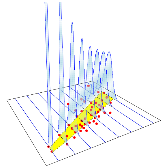
We have seen previously that the linear relation $\eta_{i}=p_{i}$ is not workable because we require $0 \leq p_{i} \leq 1$. Instead we shall use a link function $g$ such that $\eta_{i}=g\left(p_{i}\right)$. We need $g$ to be monotone and be such that $0 \leq g^{-1}(\eta) \leq 1$ for any $\eta$. The most popular choice of link function in this situation is the logit. It is defined so that:
$$
\eta=\log (p /(1-p))
$$
or equivalently:
$$
p=\frac{e^{\eta}}{1+e^{\eta}}
$$
Combining the use of the logit link with a linear predictor gives us the term logistic regression. Other choices of link function are possible but we will defer discussion of these until later. The logit and its inverse are defined as logit and ilogit in the faraway package. The relationship between $p$ and the linear predictor $\eta$ is shown in

假设检验代写

统计代写| 广义线性模型project代写Generalized Linear Model代考|Heart Disease Example

哪些因素会影响患心脏病的几率？最早
解决这一问题的研究之一始于 1960 年，使用了
来自旧金山地区的 3154 名年龄在 39 至 59 岁之间的健康男性。在研究开始时，所有人都没有心脏病。
八年半后，该研究记录了这些男性现在是否患有
心脏病以及许多其他可能与
患这种疾病的机会有关的变量。
我们从Rosenman 等人描述的西方合作小组研究中加载了这些数据的一个子集。(1975):
data(wcgs, package=”faraway”)
我们首先关注数据集中的三个变量：
summary(wcgs[,c(“chd”,”height”,”cigs”)])
chd高度香烟

没有：2897 分钟。:60.0 分钟 : 0.0
是的: 257 1st Qu.:68.0 1st Qu.: 0.0
Median :70.0 Median : 0.0
Mean :69.8 Mean :11.6
3rd Qu.:72.0 3rd Qu.:20.0

图中的第一个面板2.1显示箱线图。这显示了患有和不患有心脏病的两组男性的身高分布相似。但是心脏病是响应变量，所以我们可能更喜欢这样对待它的情节。我们将疾病的缺席/存在转换为数字0/1变量并将其绘制在图 2.1 的第二个面板中。因为高度以英寸为整数，并且响应只能取两个值，所以在每个点上添加少量噪声（称为抖动）是明智的，这样我们就可以区分它们。我们再次可以看到分布的相似性。我们可能会考虑为该图拟合一条线。

统计代写| 广义线性模型project代写Generalized Linear Model代考|Logistic Regression

假设我们有一个响应变量和一世为了一世=1,…,n它采用零或一的值磷(和一世=1)=p一世. 该响应可能与一组q预测因子(X一世1,…,X一世q). 我们需要一个模型来描述X1,…,Xq到概率p. 遵循线性模型方法，我们构建了一个线性预测器：
这一世=b0+b1X一世1+⋯+bqX一世q
由于线性预测器可以通过使用虚拟变量来适应定量和定性预测器，并且还允许原始预测器的转换和组合，因此它非常灵活并且保留了可解释性。我们可以仅通过线性预测器来表达预测器对响应的影响的想法很重要。这个想法可以扩展到其他类型响应的模型，并且是第 8 章后面讨论的更广泛类别的广义线性模型 (GLM) 的定义特征之一。

我们之前已经看到线性关系这一世=p一世不可行，因为我们需要0≤p一世≤1. 相反，我们将使用链接功能G这样这一世=G(p一世). 我们需要G是单调的并且是这样的0≤G−1(这)≤1对于任何这. 在这种情况下，最流行的链接函数选择是 logit。它被定义为：
这=日志⁡(p/(1−p))
或等效地：
p=和这1+和这
将 logit 链接的使用与线性预测器相结合，我们得到了术语逻辑回归。链接功能的其他选择是可能的，但我们将推迟讨论这些直到稍后。logit 及其倒数在 faraway 包中定义为 logit 和 igit。之间的关系p和线性预测器这显示在

统计代写请认准statistics-lab™. statistics-lab™为您的留学生涯保驾护航。

随机过程代考

在概率论概念中，随机过程是随机变量的集合。 若一随机系统的样本点是随机函数，则称此函数为样本函数，这一随机系统全部样本函数的集合是一个随机过程。 实际应用中，样本函数的一般定义在时间域或者空间域。 随机过程的实例如股票和汇率的波动、语音信号、视频信号、体温的变化，随机运动如布朗运动、随机徘徊等等。

贝叶斯方法代考

贝叶斯统计概念及数据分析表示使用概率陈述回答有关未知参数的研究问题以及统计范式。后验分布包括关于参数的先验分布，和基于观测数据提供关于参数的信息似然模型。根据选择的先验分布和似然模型，后验分布可以解析或近似，例如，马尔科夫链蒙特卡罗 (MCMC) 方法之一。贝叶斯统计概念及数据分析使用后验分布来形成模型参数的各种摘要，包括点估计，如后验平均值、中位数、百分位数和称为可信区间的区间估计。此外，所有关于模型参数的统计检验都可以表示为基于估计后验分布的概率报表。

广义线性模型代写

广义线性模型（GLM）归属统计学领域，是一种应用灵活的线性回归模型。该模型允许因变量的偏差分布有除了正态分布之外的其它分布。

statistics-lab作为专业的留学生服务机构，多年来已为美国、英国、加拿大、澳洲等留学热门地的学生提供专业的学术服务，包括但不限于Essay代写，Assignment代写，Dissertation代写，Report代写，小组作业代写，Proposal代写，Paper代写，Presentation代写，计算机作业代写，论文修改和润色，网课代做，exam代考等等。写作范围涵盖高中，本科，研究生等海外留学全阶段，辐射金融，经济学，会计学，审计学，管理学等全球99%专业科目。写作团队既有专业英语母语作者，也有海外名校硕博留学生，每位写作老师都拥有过硬的语言能力，专业的学科背景和学术写作经验。我们承诺100%原创，100%专业，100%准时，100%满意。

机器学习代写

随着AI的大潮到来，Machine Learning逐渐成为一个新的学习热点。同时与传统CS相比，Machine Learning在其他领域也有着广泛的应用，因此这门学科成为不仅折磨CS专业同学的“小恶魔”，也是折磨生物、化学、统计等其他学科留学生的“大魔王”。学习Machine learning的一大绊脚石在于使用语言众多，跨学科范围广，所以学习起来尤其困难。但是不管你在学习Machine Learning时遇到任何难题，StudyGate专业导师团队都能为你轻松解决。

多元统计分析代考

基础数据: $N$ 个样本， $P$ 个变量数的单样本，组成的横列的数据表
变量定性: 分类和顺序；变量定量：数值
数学公式的角度分为: 因变量与自变量

时间序列分析代写

随机过程，是依赖于参数的一组随机变量的全体，参数通常是时间。 随机变量是随机现象的数量表现，其时间序列是一组按照时间发生先后顺序进行排列的数据点序列。通常一组时间序列的时间间隔为一恒定值（如1秒，5分钟，12小时，7天，1年），因此时间序列可以作为离散时间数据进行分析处理。研究时间序列数据的意义在于现实中，往往需要研究某个事物其随时间发展变化的规律。这就需要通过研究该事物过去发展的历史记录，以得到其自身发展的规律。

回归分析代写

多元回归分析渐进（Multiple Regression Analysis Asymptotics）属于计量经济学领域，主要是一种数学上的统计分析方法，可以分析复杂情况下各影响因素的数学关系，在自然科学、社会和经济学等多个领域内应用广泛。

MATLAB代写

MATLAB 是一种用于技术计算的高性能语言。它将计算、可视化和编程集成在一个易于使用的环境中，其中问题和解决方案以熟悉的数学符号表示。典型用途包括：数学和计算算法开发建模、仿真和原型制作数据分析、探索和可视化科学和工程图形应用程序开发，包括图形用户界面构建MATLAB 是一个交互式系统，其基本数据元素是一个不需要维度的数组。这使您可以解决许多技术计算问题，尤其是那些具有矩阵和向量公式的问题，而只需用 C 或 Fortran 等标量非交互式语言编写程序所需的时间的一小部分。MATLAB 名称代表矩阵实验室。MATLAB 最初的编写目的是提供对由 LINPACK 和 EISPACK 项目开发的矩阵软件的轻松访问，这两个项目共同代表了矩阵计算软件的最新技术。MATLAB 经过多年的发展，得到了许多用户的投入。在大学环境中，它是数学、工程和科学入门和高级课程的标准教学工具。在工业领域，MATLAB 是高效研究、开发和分析的首选工具。MATLAB 具有一系列称为工具箱的特定于应用程序的解决方案。对于大多数 MATLAB 用户来说非常重要，工具箱允许您学习和应用专业技术。工具箱是 MATLAB 函数（M 文件）的综合集合，可扩展 MATLAB 环境以解决特定类别的问题。可用工具箱的领域包括信号处理、控制系统、神经网络、模糊逻辑、小波、仿真等。