如果你也在 怎样代写广义线性模型Generalized Linear Model这个学科遇到相关的难题，请随时右上角联系我们的24/7代写客服。在統計學上，廣義線性模型(generalized linear model，缩写作GLM) 是一種應用灵活的線性迴歸模型。该模型允许因变量的偏差分布有除了正态分布之外的其它分布。

statistics-lab™ 为您的留学生涯保驾护航 在代写广义线性模型Generalized Linear Model方面已经树立了自己的口碑, 保证靠谱, 高质且原创的统计Statistics代写服务。我们的专家在代写广义线性模型Generalized Linear Model代写方面经验极为丰富，各种代写广义线性模型Generalized Linear Model相关的作业也就用不着 说。

我们提供的代写广义线性模型Generalized Linear Model及其相关学科的代写，服务范围广, 其中包括但不限于:

• 极大似然 Maximum likelihood
• 贝叶斯方法 Bayesian methods
• 线性回归 Linear regression
• 多项式Lo​​gistic回归 Multinomial regression
• 采样理论 sampling theory

统计代写| 广义线性模型project代写Generalized Linear Model代考|Joint Model Specification

Joint Model Specification: We use the standard GLM approach for the mean:
$$
E Y_{i}=\mu_{i} \quad \eta_{i}=g\left(\mu_{i}\right)=\sum_{j} x_{i j} \beta_{j} \quad \text { var } Y_{i}=\phi_{i} V\left(\mu_{i}\right) \quad w_{i}=1 / \phi_{i}
$$
Now the dispersion, $\phi_{i}$, is no longer considered fixed. Suppose we find an estimate, $d_{i}$, of the dispersion and model it using a gamma GLM:
$$
E d_{i}=\phi_{i} \quad \zeta_{i}=\log \left(\phi_{i}\right)=\sum_{j} z_{i j} \gamma_{j} \quad \operatorname{var} d_{i}=\tau \phi_{i}^{2}
$$
Notice the connection between the two models. The model for the mean produces the response for the model for the dispersion, which in turn produces the weights for the mean model. In principle, something other than a gamma GLM could be used for the dispersion, although since we wish to model a strictly positive, continuous and typically skewed dispersion, the gamma is the obvious choice. The dispersion predictors $Z$ are usually a subset of the mean model predictors $X$.

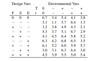
For unreplicated experiments, $r_{P}^{2}$ and $r_{D}^{2}$ are two possible choices for $d_{i}$. If replications are available, then a more direct estimate of dispersion would be possible. For more details on the formulation, estimation and inference for these kinds of model, see McCullagh and Nelder (1989), Box and Meyer (1986), Bergman and Hynen (1997) and Nelder et al. (1998).

In the last three citations, data from a welding-strength experiment was analyzed. There were nine two-level factors and 16 unreplicated runs. Previous analyses have differed on which factors are significant for the mean. We found that two factors, Drying and Material, were apparently strongly significant, while the significance of others, including Preheating, was less clear. We fit a linear model for the mean using these three predictors:

统计代写| 广义线性模型project代写Generalized Linear Model代考|Tweedie GLM

In Section $8.1$, we derived the mean and variance for an exponential (dispersion) family as

The variance function $V(\mu)=b^{\prime \prime}(\theta)$ defines how the variance is connected to the mean. We can essentially define the distribution by specifying the variance function since $\mu$ can be derived from this. Suppose we consider variance functions of the form $V(\mu)=\mu^{p}$. We have already seen four examples: the Gaussian $(p=0)$, the Poisson $(p=1)$, the gamma $(p=2)$ and the inverse Gaussian $(p=3)$.

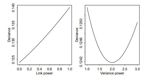
We could take the quasi-likelihood approach and simply choose the link and the variance functions as demonstrated in the previous section. We can specify our chosen link and variance and use the quasi family in fitting the $g l \mathrm{~m}$ (). Unfortunately, only the four values of $p=0,1,2,3$ are pre-programmed in base R. For these four choices, it is usually more convenient to use the one of the four distributional GLMs rather than the quasi model since we have the advantage of a full rather than quasilikelihood. We could use other, perhaps noninteger values of $p$ as demonstrated earlier but it is difficult to interpret such choices meaningfully.

Fortunately, any choice of $p$, except for the open interval $(0,1)$, defines a socalled Tweedie distribution. Values of $p$ in the interval $(1,2)$ are particularly interesting since these result in a compound Poisson-Gamma distribution. Observations from this distribution are generated as the sum of a Poisson number of gamma distributed variables in the following manner:
$Y=\sum_{i=1}^{N} X_{i}, \quad N \sim$ Poisson and, independently, $X_{i} \sim$ Gamma
The mean of the Poisson is given by $\mu^{2-p} /((2-p) \phi)$. The gamma variables have shape parameter $(2-p) /(p-1)$ and scale parameter $\phi(p-1) \mu^{p-1}$.

假设检验代写

统计代写| 广义线性模型project代写Generalized Linear Model代考|Joint Model Specification

联合模型规范：我们使用标准 GLM 方法来计算平均值：
和和一世=μ一世这一世=G(μ一世)=∑jX一世jbj 在哪里 和一世=φ一世五(μ一世)在一世=1/φ一世
现在分散，φ一世, 不再被认为是固定的。假设我们找到一个估计，d一世, 的色散并使用伽马 GLM 对其进行建模：
和d一世=φ一世G一世=日志⁡(φ一世)=∑j和一世jCj在哪里⁡d一世=τφ一世2
注意两个模型之间的联系。均值模型产生离散模型的响应，进而产生均值模型的权重。原则上，伽马 GLM 以外的其他东西也可用于色散，尽管由于我们希望模拟严格的正、连续且通常偏斜的色散，伽马是显而易见的选择。色散预测器和通常是平均模型预测变量的子集X.

对于非重复实验，r磷2和rD2是两种可能的选择d一世. 如果可以进行复制，则可以更直接地估计离散度。有关此类模型的制定、估计和推断的更多详细信息，请参见 McCullagh 和 Nelder (1989)、Box 和 Meyer (1986)、Bergman 和 Hynen (1997) 以及 Nelder 等人。（1998 年）。

在最后三个引文中，分析了焊接强度实验的数据。有 9 个二级因子和 16 个非重复运行。以前的分析在哪些因素对平均值显着方面存在差异。我们发现干燥和材料这两个因素显然非常重要，而其他因素（包括预热）的重要性则不太清楚。我们使用这三个预测变量拟合均值的线性模型：

统计代写| 广义线性模型project代写Generalized Linear Model代考|Tweedie GLM

在部分8.1，我们得出指数（离散）族的均值和方差为

方差函数五(μ)=b′′(θ)定义方差如何与均值相关联。我们基本上可以通过指定方差函数来定义分布，因为μ可以由此得出。假设我们考虑形式的方差函数五(μ)=μp. 我们已经看到了四个例子：高斯(p=0), 泊松(p=1), 伽马(p=2)和逆高斯(p=3).

我们可以采用准似然方法，并简单地选择链接和方差函数，如上一节所示。我们可以指定我们选择的链接和方差，并使用准族来拟合G一世 米()。不幸的是，只有四个值p=0,1,2,3在基础 R 中预编程。对于这四种选择，通常使用四种分布 GLM 中的一种而不是准模型更方便，因为我们具有完全而不是准似然的优势。我们可以使用其他的，也许是非整数值p如前所述，但很难有意义地解释这些选择。

幸运的是，任何选择p, 除了开区间(0,1), 定义了一个所谓的 Tweedie 分布。的价值观p在区间(1,2)特别有趣，因为这些会导致复合 Poisson-Gamma 分布。来自该分布的观测值以下列方式生成为伽马分布变量的泊松数之和：
和=∑一世=1ñX一世,ñ∼泊松，并且独立地，X一世∼Gamma
泊松的平均值由下式给出μ2−p/((2−p)φ). 伽玛变量具有形状参数(2−p)/(p−1)和尺度参数φ(p−1)μp−1.

统计代写请认准statistics-lab™. statistics-lab™为您的留学生涯保驾护航。

随机过程代考

在概率论概念中，随机过程是随机变量的集合。 若一随机系统的样本点是随机函数，则称此函数为样本函数，这一随机系统全部样本函数的集合是一个随机过程。 实际应用中，样本函数的一般定义在时间域或者空间域。 随机过程的实例如股票和汇率的波动、语音信号、视频信号、体温的变化，随机运动如布朗运动、随机徘徊等等。

贝叶斯方法代考

贝叶斯统计概念及数据分析表示使用概率陈述回答有关未知参数的研究问题以及统计范式。后验分布包括关于参数的先验分布，和基于观测数据提供关于参数的信息似然模型。根据选择的先验分布和似然模型，后验分布可以解析或近似，例如，马尔科夫链蒙特卡罗 (MCMC) 方法之一。贝叶斯统计概念及数据分析使用后验分布来形成模型参数的各种摘要，包括点估计，如后验平均值、中位数、百分位数和称为可信区间的区间估计。此外，所有关于模型参数的统计检验都可以表示为基于估计后验分布的概率报表。

广义线性模型代考

广义线性模型（GLM）归属统计学领域，是一种应用灵活的线性回归模型。该模型允许因变量的偏差分布有除了正态分布之外的其它分布。

statistics-lab作为专业的留学生服务机构，多年来已为美国、英国、加拿大、澳洲等留学热门地的学生提供专业的学术服务，包括但不限于Essay代写，Assignment代写，Dissertation代写，Report代写，小组作业代写，Proposal代写，Paper代写，Presentation代写，计算机作业代写，论文修改和润色，网课代做，exam代考等等。写作范围涵盖高中，本科，研究生等海外留学全阶段，辐射金融，经济学，会计学，审计学，管理学等全球99%专业科目。写作团队既有专业英语母语作者，也有海外名校硕博留学生，每位写作老师都拥有过硬的语言能力，专业的学科背景和学术写作经验。我们承诺100%原创，100%专业，100%准时，100%满意。

机器学习代写

随着AI的大潮到来，Machine Learning逐渐成为一个新的学习热点。同时与传统CS相比，Machine Learning在其他领域也有着广泛的应用，因此这门学科成为不仅折磨CS专业同学的“小恶魔”，也是折磨生物、化学、统计等其他学科留学生的“大魔王”。学习Machine learning的一大绊脚石在于使用语言众多，跨学科范围广，所以学习起来尤其困难。但是不管你在学习Machine Learning时遇到任何难题，StudyGate专业导师团队都能为你轻松解决。

多元统计分析代考

基础数据: $N$ 个样本， $P$ 个变量数的单样本，组成的横列的数据表
变量定性: 分类和顺序；变量定量：数值
数学公式的角度分为: 因变量与自变量

时间序列分析代写

随机过程，是依赖于参数的一组随机变量的全体，参数通常是时间。 随机变量是随机现象的数量表现，其时间序列是一组按照时间发生先后顺序进行排列的数据点序列。通常一组时间序列的时间间隔为一恒定值（如1秒，5分钟，12小时，7天，1年），因此时间序列可以作为离散时间数据进行分析处理。研究时间序列数据的意义在于现实中，往往需要研究某个事物其随时间发展变化的规律。这就需要通过研究该事物过去发展的历史记录，以得到其自身发展的规律。

回归分析代写

多元回归分析渐进（Multiple Regression Analysis Asymptotics）属于计量经济学领域，主要是一种数学上的统计分析方法，可以分析复杂情况下各影响因素的数学关系，在自然科学、社会和经济学等多个领域内应用广泛。

MATLAB代写

MATLAB 是一种用于技术计算的高性能语言。它将计算、可视化和编程集成在一个易于使用的环境中，其中问题和解决方案以熟悉的数学符号表示。典型用途包括：数学和计算算法开发建模、仿真和原型制作数据分析、探索和可视化科学和工程图形应用程序开发，包括图形用户界面构建MATLAB 是一个交互式系统，其基本数据元素是一个不需要维度的数组。这使您可以解决许多技术计算问题，尤其是那些具有矩阵和向量公式的问题，而只需用 C 或 Fortran 等标量非交互式语言编写程序所需的时间的一小部分。MATLAB 名称代表矩阵实验室。MATLAB 最初的编写目的是提供对由 LINPACK 和 EISPACK 项目开发的矩阵软件的轻松访问，这两个项目共同代表了矩阵计算软件的最新技术。MATLAB 经过多年的发展，得到了许多用户的投入。在大学环境中，它是数学、工程和科学入门和高级课程的标准教学工具。在工业领域，MATLAB 是高效研究、开发和分析的首选工具。MATLAB 具有一系列称为工具箱的特定于应用程序的解决方案。对于大多数 MATLAB 用户来说非常重要，工具箱允许您学习和应用专业技术。工具箱是 MATLAB 函数（M 文件）的综合集合，可扩展 MATLAB 环境以解决特定类别的问题。可用工具箱的领域包括信号处理、控制系统、神经网络、模糊逻辑、小波、仿真等。