如果你也在 怎样代写机器学习machine learning这个学科遇到相关的难题,请随时右上角联系我们的24/7代写客服。
机器学习(ML)是人工智能(AI)的一种类型,它允许软件应用程序在预测结果时变得更加准确,而无需明确编程。机器学习算法使用历史数据作为输入来预测新的输出值。
statistics-lab™ 为您的留学生涯保驾护航 在代写机器学习machine learning方面已经树立了自己的口碑, 保证靠谱, 高质且原创的统计Statistics代写服务。我们的专家在代写机器学习machine learning代写方面经验极为丰富,各种代写机器学习machine learning相关的作业也就用不着说。
我们提供的机器学习machine learning及其相关学科的代写,服务范围广, 其中包括但不限于:
- Statistical Inference 统计推断
- Statistical Computing 统计计算
- Advanced Probability Theory 高等概率论
- Advanced Mathematical Statistics 高等数理统计学
- (Generalized) Linear Models 广义线性模型
- Statistical Machine Learning 统计机器学习
- Longitudinal Data Analysis 纵向数据分析
- Foundations of Data Science 数据科学基础
计算机代写|机器学习代写machine learning代考|Notation
We employ lowercase letters $x, s, v, \cdots$ in order to describe variables that can lie in specific domains such as real numbers $\mathbb{R}$, real positive $\mathbb{R}^{+}$, integers $\mathbb{Z}$, closed intervals $[\cdot,$, , open intervals (,$\left.\cdot\right)$, and so on. Often, the problems studied involve multiple variables that can be regrouped in arrays. A 1-D array or vector containing scalars is represented as
$$
\mathbf{x}=\left[\begin{array}{c}
x_{1} \
x_{2} \
\vdots \
x_{n}
\end{array}\right]
$$
By convention, a vector $\mathbf{x}$ implicitly refers to a $n \times 1$ column vector. For example, if each element $x_{i} \equiv[\mathbf{x}]{i}$ is a real number $[\mathbf{x}]{i} \in \mathbb{R}$ for all $i$ from 1 to $n$, then the vector belongs to the $n$-dimensional real domain $\mathbb{R}^{n}$. This last statement can be expressed mathematically as $[\mathbf{x}]{i} \in \mathbb{R}, \forall i \in{1: n} \rightarrow \mathbf{x} \in \mathbb{R}^{n}$. In machine learning, it is common to have 2-D arrays or matrices, $$ \mathbf{X}=\left[\begin{array}{cccc} x{11} & x_{12} & \cdots & x_{1 n} \
x_{21} & x_{22} & \cdots & x_{2 n} \
\vdots & \vdots & \ddots & \vdots \
x_{m 1} & x_{m 2} & \cdots & x_{m n}
\end{array}\right]
$$
where, for example, if each $x_{i j} \equiv[\mathbf{X}]_{i j} \in \mathbb{R}, \forall i \in{1: m}, j \in{1:$ $n} \rightarrow \mathbf{X} \in \mathbb{R}^{m \times n}$. Arrays beyond two dimensions are referred to as tensors. Although tensors are widely employed in the field of neural networks, they will not be treated in this book.
There are several matrices with specific properties: A diagona. matrix is square and has only terms on its main diagonal.
$$
\mathbf{Y}=\operatorname{diag}(\mathbf{x})=\left[\begin{array}{cccc}
x_{1} & 0 & \cdots & 0 \
0 & x_{2} & \cdots & 0 \
\vdots & \vdots & \ddots & \vdots \
0 & 0 & \cdots & x_{n}
\end{array}\right]{n \times n} $$ An identity matrix $\mathbf{I}$ is similar to a diagonal matrix except that elements on the main diagonal are 1 , and 0 everywhere else, $$ \mathbf{I}=\left[\begin{array}{cccc} 1 & 0 & \cdots & 0 \ 0 & 1 & \cdots & 0 \ \vdots & \vdots & \ddots & \vdots \ 0 & 0 & \cdots & 1 \end{array}\right]{n \times n}
$$
A block diagonal matrix concatenates several matrices on the ma diagonal of a single matrix,
$$
\operatorname{blkdiag}(\mathbf{A}, \mathbf{B})=\left[\begin{array}{lr}
\mathbf{A} & \mathbf{0} \
\mathbf{0} & \mathbf{B}
\end{array}\right] \text {. }
$$
We can manipulate the dimensions of matrices using the transposition operation so that indices are permuted $\left[\mathbf{X}^{\top}\right]{i j}=[\mathbf{X}]{j i}$. For example,
$$
\mathbf{X}=\left[\begin{array}{lll}
x_{11} & x_{12} & x_{13} \
x_{21} & x_{22} & x_{23}
\end{array}\right] \rightarrow \mathbf{X}^{\boldsymbol{\top}}=\left[\begin{array}{ll}
x_{11} & x_{21} \
x_{12} & x_{22} \
x_{13} & x_{23}
\end{array}\right]
$$
The trace of a square matrix $\mathbf{X}$ corresponds to the sum of the elements on its main diagonal,
$$
\operatorname{tr}(\mathbf{X})=\sum_{i=1}^{n} x_{i i}
$$
计算机代写|机器学习代写machine learning代考|Operations
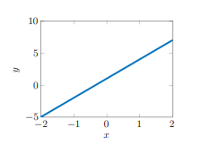
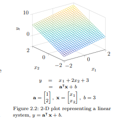
In the context of machine learning, linear algebra is employed because of its capacity to model linear systems of equations in a format that is compact and well suited for computer calculations. In a 1-D case, such as the one represented in figure 2.1, the $x$ space is mapped into the $y$ space, $\mathbb{R} \rightarrow \mathbb{R}$, through a linear (i.e., affine) function. Figure $2.2$ presents an example of a 2-D linear function where the $\mathbf{x}$ space is mapped into the $y$ space, $\mathbb{R}^{2} \rightarrow \mathbb{R}$. This can be generalized to linear systems $\mathbf{y}=\mathbf{A x}+\mathbf{b}$, defining a mapping so that $\mathbb{R}^{n} \rightarrow \mathbb{R}^{m}$, where $\mathbf{x}$ and $\mathbf{y}$ are respectively $n \times 1$ and $m \times 1$
vectors. The product of the matrix $\mathbf{A}$ with the vector $\mathbf{x}$ is defined as $[\mathbf{A x}]{i}=\sum{j}[\mathbf{A}]{i j} \cdot[\mathbf{x}]{j}$.
In more general cases, linear algebra is employed to multiply a matrix A of size $n \times k$ with another matrix $\mathbf{B}$ of size $k \times m$, so the result is a $n \times m$ matrix,
$$
\begin{aligned}
\mathbf{C} &=\mathbf{A B} \
&=\mathbf{A} \times \mathbf{B}
\end{aligned}
$$
The matrix multiplication operation follows $[\mathbf{C}]{i j}=\sum{k}[\mathbf{A}]{i k} \cdot[\mathbf{B}]{k j}$, as illustrated in figure $2.3$. Following the requirement on the size of the matrices multiplied, this operation is not generally commutative so that $\mathbf{A B} \neq \mathbf{B A}$. Matrix multiplication follows several properties such as the following:
Distributivity
$\begin{aligned} \mathbf{A}(\mathbf{B}+\mathbf{C}) &=\mathbf{A B}+\mathbf{A} \mathbf{C} \ \mathbf{A}(\mathbf{B} \mathbf{C}) &=(\mathbf{A B}) \mathbf{C} \(\mathbf{A B})^{\top} &=\mathbf{B}^{\boldsymbol{\top}} \mathbf{A}^{\top} . \end{aligned}$
When the matrix multiplication operator is applied to $n \times 1$ vectors, it reduces to the inner product,
$$
\begin{aligned}
\mathbf{x}^{\boldsymbol{\top}} \mathbf{y} & \equiv \mathbf{x} \cdot \mathbf{y} \
&=\left[\begin{array}{lll}
x_{1} & \cdots & x_{n}
\end{array}\right] \times\left[\begin{array}{c}
y_{1} \
\vdots \
y_{n}
\end{array}\right] \
&=\sum_{\mathbf{i}=1}^{n} x_{i} y_{k}
\end{aligned}
$$
Another common operation is the Hadamar product or elementwise product, which is represented by the symbol $\odot$. It consists in multiplying each term from matrices $\mathbf{A}{m \times n}$ and $\mathbf{B}{m \times n}$ in order to obtain $\mathbf{C}{m \times n}$, $$ \begin{aligned} \mathbf{C} &=\mathbf{A} \odot \mathbf{B} \ {[\mathbf{C}]{i j} } &=[\mathbf{A}]{i j} \cdot[\mathbf{B}]{i j}
\end{aligned}
$$
计算机代写|机器学习代写machine learning代考|Norms
Norms measure how large a vector is. In a generic way, the $L^{\rho}$-norm is defined as
$$
|\mathbf{x}|_{p}=\left(\sum_{i}\left|[\mathbf{x}]{i}\right|^{p}\right)^{1 / p} $$ Special cases of interest are $$ \begin{array}{ll} |\mathbf{x}|{2}=\sqrt{\sum_{i}[\mathbf{x}]{i}^{2}} \equiv \sqrt{\mathbf{x}^{\top} \mathbf{x}} & \text { (Euclidian norm) } \ |\mathbf{x}|{1}=\sum_{i}\left|[\mathbf{x}]{i}\right| & \text { (Manhattan norm) } \ |\mathbf{x}|{\infty}=\max {i}\left|[\mathbf{x}]{i}\right| . & (\text { Max norm) }
\end{array}
$$
These cases are illustrated in figure 2.4. Among all cases, the $L^{2}$ norm (Euclidian distance) is the most common. For example, \$.1.1 presents for the context of linear regression how choosing a Euclidian norm to measure the distance between observations and model predictions allows solving the parameter estimation problem analytically.
机器学习代考
计算机代写|机器学习代写machine learning代考|Notation
我们使用小写字母X,s,在,⋯为了描述可以位于特定域中的变量,例如实数R, 真阳性R+, 整数从, 闭区间[⋅,, , 开区间 (,⋅), 等等。通常,所研究的问题涉及可以在数组中重新组合的多个变量。包含标量的一维数组或向量表示为
X=[X1 X2 ⋮ Xn]
按照惯例,向量X隐含地提到一个n×1列向量。例如,如果每个元素X一世≡[X]一世是一个实数[X]一世∈R对所有人一世从 1 到n,则该向量属于n维实域Rn. 最后一条语句可以在数学上表示为[X]一世∈R,∀一世∈1:n→X∈Rn. 在机器学习中,通常有二维数组或矩阵,
X=[X11X12⋯X1n X21X22⋯X2n ⋮⋮⋱⋮ X米1X米2⋯X米n]
例如,如果每个X一世j≡[X]一世j∈R,∀一世∈1:米,j∈1:$$n→X∈R米×n. 超出二维的数组称为张量。虽然张量在神经网络领域得到了广泛的应用,但本书不会对其进行讨论。
有几个具有特定属性的矩阵: 对角线。矩阵是正方形的,并且在其主对角线上只有项。
是=诊断(X)=[X10⋯0 0X2⋯0 ⋮⋮⋱⋮ 00⋯Xn]n×n单位矩阵我类似于对角矩阵,除了主对角线上的元素是 1 ,其他地方都是 0,
我=[10⋯0 01⋯0 ⋮⋮⋱⋮ 00⋯1]n×n
块对角矩阵在单个矩阵的 ma 对角线上连接多个矩阵,
诊断(一个,乙)=[一个0 0乙].
我们可以使用转置操作来操纵矩阵的维数,以便排列索引[X⊤]一世j=[X]j一世. 例如,
X=[X11X12X13 X21X22X23]→X⊤=[X11X21 X12X22 X13X23]
方阵的迹X对应于其主对角线上的元素之和,
tr(X)=∑一世=1nX一世一世
计算机代写|机器学习代写machine learning代考|Operations
在机器学习的背景下,使用线性代数是因为它能够以紧凑且非常适合计算机计算的格式对线性方程组进行建模。在一维情况下,如图 2.1 所示,X空间被映射到是空间,R→R,通过一个线性(即仿射)函数。数字2.2给出了一个二维线性函数的例子,其中X空间被映射到是空间,R2→R. 这可以推广到线性系统是=一个X+b,定义一个映射,使得Rn→R米, 在哪里X和是分别是n×1和米×1
向量。矩阵的乘积一个与向量X定义为[一个X]一世=∑j[一个]一世j⋅[X]j.
在更一般的情况下,使用线性代数来乘以大小为 A 的矩阵n×ķ与另一个矩阵乙大小的ķ×米,所以结果是n×米矩阵,
C=一个乙 =一个×乙
矩阵乘法运算如下[C]一世j=∑ķ[一个]一世ķ⋅[乙]ķj, 如图2.3. 遵循对矩阵大小相乘的要求,此操作通常不是可交换的,因此一个乙≠乙一个. 矩阵乘法遵循以下几个属性:
分布性
一个(乙+C)=一个乙+一个C 一个(乙C)=(一个乙)C\(一个乙)⊤=乙⊤一个⊤.
当矩阵乘法运算符应用于n×1向量,它减少到内积,
X⊤是≡X⋅是 =[X1⋯Xn]×[是1 ⋮ 是n] =∑一世=1nX一世是ķ
另一种常见的操作是 Hadamar 乘积或元素乘积,用符号表示⊙. 它包括将矩阵中的每个项相乘一个米×n和乙米×n为了得到C米×n,
C=一个⊙乙 [C]一世j=[一个]一世j⋅[乙]一世j
计算机代写|机器学习代写machine learning代考|Norms
范数衡量一个向量有多大。以一般的方式,大号ρ-norm 定义为
|X|p=(∑一世|[X]一世|p)1/p感兴趣的特殊情况是
|X|2=∑一世[X]一世2≡X⊤X (欧几里得范数) |X|1=∑一世|[X]一世| (曼哈顿规范) |X|∞=最大限度一世|[X]一世|.( 最大标准)
这些情况如图 2.4 所示。在所有案例中,大号2范数(欧几里得距离)是最常见的。例如,$ .1.1 为线性回归的上下文提供了如何选择欧几里得范数来测量观测值和模型预测之间的距离,从而可以分析地解决参数估计问题。

统计代写请认准statistics-lab™. statistics-lab™为您的留学生涯保驾护航。
金融工程代写
金融工程是使用数学技术来解决金融问题。金融工程使用计算机科学、统计学、经济学和应用数学领域的工具和知识来解决当前的金融问题,以及设计新的和创新的金融产品。
非参数统计代写
非参数统计指的是一种统计方法,其中不假设数据来自于由少数参数决定的规定模型;这种模型的例子包括正态分布模型和线性回归模型。
广义线性模型代考
广义线性模型(GLM)归属统计学领域,是一种应用灵活的线性回归模型。该模型允许因变量的偏差分布有除了正态分布之外的其它分布。
术语 广义线性模型(GLM)通常是指给定连续和/或分类预测因素的连续响应变量的常规线性回归模型。它包括多元线性回归,以及方差分析和方差分析(仅含固定效应)。
有限元方法代写
有限元方法(FEM)是一种流行的方法,用于数值解决工程和数学建模中出现的微分方程。典型的问题领域包括结构分析、传热、流体流动、质量运输和电磁势等传统领域。
有限元是一种通用的数值方法,用于解决两个或三个空间变量的偏微分方程(即一些边界值问题)。为了解决一个问题,有限元将一个大系统细分为更小、更简单的部分,称为有限元。这是通过在空间维度上的特定空间离散化来实现的,它是通过构建对象的网格来实现的:用于求解的数值域,它有有限数量的点。边界值问题的有限元方法表述最终导致一个代数方程组。该方法在域上对未知函数进行逼近。[1] 然后将模拟这些有限元的简单方程组合成一个更大的方程系统,以模拟整个问题。然后,有限元通过变化微积分使相关的误差函数最小化来逼近一个解决方案。
tatistics-lab作为专业的留学生服务机构,多年来已为美国、英国、加拿大、澳洲等留学热门地的学生提供专业的学术服务,包括但不限于Essay代写,Assignment代写,Dissertation代写,Report代写,小组作业代写,Proposal代写,Paper代写,Presentation代写,计算机作业代写,论文修改和润色,网课代做,exam代考等等。写作范围涵盖高中,本科,研究生等海外留学全阶段,辐射金融,经济学,会计学,审计学,管理学等全球99%专业科目。写作团队既有专业英语母语作者,也有海外名校硕博留学生,每位写作老师都拥有过硬的语言能力,专业的学科背景和学术写作经验。我们承诺100%原创,100%专业,100%准时,100%满意。
随机分析代写
随机微积分是数学的一个分支,对随机过程进行操作。它允许为随机过程的积分定义一个关于随机过程的一致的积分理论。这个领域是由日本数学家伊藤清在第二次世界大战期间创建并开始的。
时间序列分析代写
随机过程,是依赖于参数的一组随机变量的全体,参数通常是时间。 随机变量是随机现象的数量表现,其时间序列是一组按照时间发生先后顺序进行排列的数据点序列。通常一组时间序列的时间间隔为一恒定值(如1秒,5分钟,12小时,7天,1年),因此时间序列可以作为离散时间数据进行分析处理。研究时间序列数据的意义在于现实中,往往需要研究某个事物其随时间发展变化的规律。这就需要通过研究该事物过去发展的历史记录,以得到其自身发展的规律。
回归分析代写
多元回归分析渐进(Multiple Regression Analysis Asymptotics)属于计量经济学领域,主要是一种数学上的统计分析方法,可以分析复杂情况下各影响因素的数学关系,在自然科学、社会和经济学等多个领域内应用广泛。
MATLAB代写
MATLAB 是一种用于技术计算的高性能语言。它将计算、可视化和编程集成在一个易于使用的环境中,其中问题和解决方案以熟悉的数学符号表示。典型用途包括:数学和计算算法开发建模、仿真和原型制作数据分析、探索和可视化科学和工程图形应用程序开发,包括图形用户界面构建MATLAB 是一个交互式系统,其基本数据元素是一个不需要维度的数组。这使您可以解决许多技术计算问题,尤其是那些具有矩阵和向量公式的问题,而只需用 C 或 Fortran 等标量非交互式语言编写程序所需的时间的一小部分。MATLAB 名称代表矩阵实验室。MATLAB 最初的编写目的是提供对由 LINPACK 和 EISPACK 项目开发的矩阵软件的轻松访问,这两个项目共同代表了矩阵计算软件的最新技术。MATLAB 经过多年的发展,得到了许多用户的投入。在大学环境中,它是数学、工程和科学入门和高级课程的标准教学工具。在工业领域,MATLAB 是高效研究、开发和分析的首选工具。MATLAB 具有一系列称为工具箱的特定于应用程序的解决方案。对于大多数 MATLAB 用户来说非常重要,工具箱允许您学习和应用专业技术。工具箱是 MATLAB 函数(M 文件)的综合集合,可扩展 MATLAB 环境以解决特定类别的问题。可用工具箱的领域包括信号处理、控制系统、神经网络、模糊逻辑、小波、仿真等。