如果你也在 怎样代写机器学习machine learning这个学科遇到相关的难题,请随时右上角联系我们的24/7代写客服。
机器学习(ML)是人工智能(AI)的一种类型,它允许软件应用程序在预测结果时变得更加准确,而无需明确编程。机器学习算法使用历史数据作为输入来预测新的输出值。
statistics-lab™ 为您的留学生涯保驾护航 在代写机器学习machine learning方面已经树立了自己的口碑, 保证靠谱, 高质且原创的统计Statistics代写服务。我们的专家在代写机器学习machine learning代写方面经验极为丰富,各种代写机器学习machine learning相关的作业也就用不着说。
我们提供的机器学习machine learning及其相关学科的代写,服务范围广, 其中包括但不限于:
- Statistical Inference 统计推断
- Statistical Computing 统计计算
- Advanced Probability Theory 高等概率论
- Advanced Mathematical Statistics 高等数理统计学
- (Generalized) Linear Models 广义线性模型
- Statistical Machine Learning 统计机器学习
- Longitudinal Data Analysis 纵向数据分析
- Foundations of Data Science 数据科学基础
计算机代写|机器学习代写machine learning代考|Discrete Random Variables
In the case where $\mathcal{S}$ is a discrete domain, the probability that $X=x$ is described by a probability mass function (PMF). In terms of notation $\operatorname{Pr}(X=x) \equiv p_{X}(x) \equiv p(x)$ are all equivalent. Moreover, we typically describe a random variable by defining its sampling space and its probability mass function so that $x: X \sim p_{X}(x)$. The symbol $\sim$ reads as distributed like. Analogously to the probability of events, the probability that $X=x$ must be
$$
0 \leq p_{X}(x) \leq 1
$$
and the sum of the probability for all $x \in \mathcal{S}$ follows
$$
\sum_{x} p_{X}(x)=1 .
$$
For the post-earthquake structural safety example introduced in $\S 3.1$, where
$$
\mathcal{S}=\left{\begin{array}{rc}
\text { no damage } & (\mathrm{N}) \
\text { light damage } & (\mathrm{L}) \
\text { important damage } & \text { (I) } \
\text { collapse } & \text { (C) }
\end{array}\right},
$$
the sampling space along with the probability of each event can be represented by a probability mass function as depicted in figure $3.10$.
The event corresponding to damages that are either light or important corresponds to $\mathrm{L} \cup \mathrm{I} \equiv{1 \leq x \leq 2}$. Because the events $x=1$ and $x=2$ are mutually exclusive, the probability
$$
\begin{aligned}
\operatorname{Pr}(\mathbf{L} \cup \mathrm{I}) &=\operatorname{Pr}({1 \leq X \leq 2}) \
&=p_{X}(x=1)+p_{X}(x=2)
\end{aligned}
$$
The probability that $X$ takes a value less than or equal to $x$ is described by a cumulative mass function (CMF),
$$
\operatorname{Pr}(X \leq x)=F_{X}(x)=\sum_{x^{\prime} \leq x} p_{X}\left(x^{\prime}\right)
$$
Figure $3.11$ presents on the same graph the probability mass function (PMF) and the cumulative mass function. As its name indicates, the CMF corresponds to the cumulative sum of the PMF. Inversely, the PMF can be obtained from the CMF following
$$
p_{X}\left(x_{i}\right)=F_{X}\left(x_{i}\right)-F_{X}\left(x_{i-1}\right) .
$$
计算机代写|机器学习代写machine learning代考|Multivariate Random Variables
It is common to study the joint occurrence of multiple phenomena. In the context of probability theory, it is done using multivariate random variables. $\mathbf{x}=\left[\begin{array}{llll}x_{1} & x_{2} & \cdots & x_{n}\end{array}\right]^{\top}$ is a vector (column) containing realizations for $n$ random variables $\mathbf{X}=\left[\left.\begin{array}{llll}X_{1} & X_{2} & \cdots & X_{n}\end{array}\right|^{\top}\right.$, $\mathbf{x}: \mathbf{X} \sim p \mathbf{x}(\mathbf{x}) \equiv p(\mathbf{x})$, or $\mathbf{x}: \mathbf{X} \sim f \mathbf{X}(\mathbf{x}) \equiv f(\mathbf{x})$. For the discrete case, the probability of the joint realization $\mathbf{x}$ is described by
$$
p_{\mathbf{X}}(\mathbf{x})=\operatorname{Pr}\left(X_{1}=x_{1} \backslash X_{2}=x_{2} \backslash \cdots \backslash X_{n}=x_{n}\right)
$$
where $0 \leq p \mathbf{x}(\mathbf{x}) \leq 1$. For the continuous case, it is
$$
f \mathbf{x}(\mathbf{x}) \Delta \mathbf{x}=\operatorname{Pr}\left(x_{1}1$ because it describes a probability density. As mentioned earlier, two random variables $X_{1}$ and $X_{2}$ are statistically independent $(\perp)$ if
$$
p_{X_{1} \mid x_{2}}\left(x_{1} \mid x_{2}\right)=p X_{1}\left(x_{1}\right) .
$$
If $X_{1} \perp X_{2} \perp \cdots \perp_{n} X$ the joint PMF is defined by the product of its marginals,
$$
p_{X_{1}: X_{n}}\left(x_{1}, \cdots, x_{n}\right)=p_{X_{1}}\left(x_{1}\right) p_{X_{2}}\left(x_{2}\right) \cdots p_{X_{n}}\left(x_{n}\right)
$$
For the general case where $X_{1}, X_{2}, \cdots, X_{n}$ are not statistically independent, their joint PMF can be defined using the chain rule,
$$
\begin{aligned}
p_{X_{1}: X_{n}}\left(x_{1}, \cdots, x_{n}\right)=& p_{X_{1} \mid X_{2}: X_{n}}\left(x_{1} \mid x_{2}, \cdots, x_{n}\right) \cdots \
\cdot p_{X_{n-1}} \mid X_{n}\left(x_{n-1} \mid x_{n}\right) \cdot p_{X_{\mathrm{n}}}\left(x_{n}\right) .
\end{aligned}
$$
The same rules apply for contimunus random variahles except. that $p_{\mathbf{X}}(\mathbf{x})$ is replaced by $f_{\mathbf{X}}(\mathbf{x})$. Figure $3.14$ presents examples of marginals and a bivariate joint probability density function.
The multivariate cumulative distribution function describes the probability that a set of $n$ random variables is simultaneously lesser or equal to $\mathbf{x}$,
$$
F_{\mathbf{x}}(\mathbf{x})=\operatorname{Pr}\left(X_{1} \leq x_{1} \backslash \cdots \backslash X_{n} \leq x_{n}\right)
$$
计算机代写|机器学习代写machine learning代考|Functions of Random Varia
Let us consider a continuous random variable $X \sim f_{X}(x)$ and a monotonic deterministic function $y=g(x)$. The function’s output $Y$ is a random variable because it takes as input the random variable $X$. The PDF $f_{Y}(y)$ is defined knowing that for each infinitesimal part of the domain $d x$, there is a corresponding $d y$, and the probability over both domains must be equal,
$$
\begin{aligned}
\operatorname{Pr}(y<Y \leq y+d y) &=\operatorname{Pr}(x<X \leq x+d x) \
\underbrace{f_{y}(y)}{\geq 0} d y &=\underbrace{f{X}(x)}{\geq 0} d x . \end{aligned} $$ The change-of-variable rule for $f{Y}(y)$ is defined by
$$
\begin{aligned}
f_{Y}(y) &=f_{X}(x)\left|\frac{d x}{d y}\right| \
&=f_{X}(x)\left|\frac{d y}{d x}\right|^{-1} \
&=f_{X}\left(g^{-1}(y)\right)\left|\frac{d g\left(g^{-1}(y)\right)}{d x}\right|^{-1}
\end{aligned}
$$
where multiplying by $\frac{d x}{d y}$ accounts for the change in the size of the neighborhood of $x$ with respect to $y$, and where the absolute value ensures that $f_{Y}(y) \geq 0$. For a function $y=g(x)$ and its inverse $x=g^{-1}(y)$, the gradient is obtained from
$$
\frac{d y}{d x} \equiv \frac{d g(x)}{d x} \equiv \frac{d g(\overbrace{\left.g^{-1}(y)\right)}^{=x}}{d x} .
$$
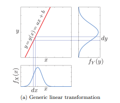
Figure $3.19$ presents an example of nonlinear transformation $y=$ $g(x)$. Notice how, because of the nonlinear transformation, the maximum for $f_{X}\left(x^{}\right)$ and the maximum for $f_{Y}\left(y^{}\right)$ do not occur for the same locations, that is, $y^{} \neq g\left(x^{}\right)$.
Given a set of $n$ random variables $\mathbf{x} \in \mathbb{R}^{n}: \mathbf{X} \sim f_{\mathbf{X}}(\mathbf{x})$, we can generalize the transformation rule for an $n$ to $n$ multivariate function $\mathbf{y}=g(\mathbf{x})$, as illustrated in figure $3.20$ a for a case where $n=2$. As with the univariate case, we need to account for the change in
the neighborhood size when going from the original to the transformed space, as illustrated in figure $3.20 \mathrm{~b}$. The transformation is then defined by
$$
\begin{aligned}
f_{\mathbf{Y}}(\mathbf{y}) d \mathbf{y} &=f_{\mathbf{X}}(\mathbf{x}) d \mathbf{x} \
f_{\mathbf{Y}}(\mathbf{y}) &=f_{\mathbf{X}}(\mathbf{x})\left|\frac{d \mathbf{x}}{d \mathbf{y}}\right|,
\end{aligned}
$$
where $\left|\frac{d \mathbf{x}}{d \mathbf{y}}\right|$ is the inverse of the determinant of the Jacobian matrix,
$$
\begin{aligned}
\left|\frac{d \mathbf{x}}{d \mathbf{y}}\right| &=\left|\operatorname{det} \mathbf{J}{\mathbf{y}, \mathbf{x}}\right|^{-1} \ \left|\frac{d \mathbf{y}}{d \mathbf{x}}\right| &=\left|\operatorname{det} \mathbf{J}{\mathbf{y}, \mathbf{x}}\right|
\end{aligned}
$$
机器学习代考
计算机代写|机器学习代写machine learning代考|Discrete Random Variables
在这种情况下小号是一个离散域,概率X=X由概率质量函数 (PMF) 描述。在符号方面公关(X=X)≡pX(X)≡p(X)都是等价的。此外,我们通常通过定义其采样空间和概率质量函数来描述随机变量,以便X:X∼pX(X). 符号∼读起来像分布式。类似于事件的概率,X=X一定是
0≤pX(X)≤1
和所有概率的总和X∈小号跟随
∑XpX(X)=1.
对于地震后结构安全的例子介绍§§3.1, 在哪里
\mathcal{S}=\left{\begin{array}{rc} \text { 无损伤 } & (\mathrm{N}) \ \text { 轻微损伤 } & (\mathrm{L}) \ \text {重要损坏 } & \text { (I) } \ \text { collapse } & \text { (C) } \end{array}\right},\mathcal{S}=\left{\begin{array}{rc} \text { 无损伤 } & (\mathrm{N}) \ \text { 轻微损伤 } & (\mathrm{L}) \ \text {重要损坏 } & \text { (I) } \ \text { collapse } & \text { (C) } \end{array}\right},
采样空间以及每个事件的概率可以用概率质量函数表示,如图所示3.10.
与轻微或重要的损害相对应的事件对应于大号∪我≡1≤X≤2. 因为事件X=1和X=2是互斥的,概率
公关(大号∪我)=公关(1≤X≤2) =pX(X=1)+pX(X=2)
的概率X取小于或等于的值X由累积质量函数 (CMF) 描述,
公关(X≤X)=FX(X)=∑X′≤XpX(X′)
数字3.11在同一图表上显示概率质量函数 (PMF) 和累积质量函数。顾名思义,CMF 对应于 PMF 的累积和。相反,PMF 可以从 CMF 中获得
pX(X一世)=FX(X一世)−FX(X一世−1).
计算机代写|机器学习代写machine learning代考|Multivariate Random Variables
研究多种现象的共同发生是很常见的。在概率论的背景下,它是使用多元随机变量完成的。X=[X1X2⋯Xn]⊤是一个包含实现的向量(列)n随机变量X=[X1X2⋯Xn|⊤, X:X∼pX(X)≡p(X), 或者X:X∼FX(X)≡F(X). 对于离散情况,联合实现的概率X描述为
pX(X)=公关(X1=X1∖X2=X2∖⋯∖Xn=Xn)
在哪里0≤pX(X)≤1. 对于连续的情况,它是
f \mathbf{x}(\mathbf{x}) \Delta \mathbf{x}=\operatorname{Pr}\left(x_{1}1$ 因为它描述了一个概率密度。如前所述,两个随机变量 $ X_{1}$ 和 $X_{2}$ 在统计上独立 $(\perp)$ 如果f \mathbf{x}(\mathbf{x}) \Delta \mathbf{x}=\operatorname{Pr}\left(x_{1}1$ 因为它描述了一个概率密度。如前所述,两个随机变量 $ X_{1}$ 和 $X_{2}$ 在统计上独立 $(\perp)$ 如果
p_{X_{1} \mid x_{2}}\left(x_{1} \mid x_{2}\right)=p X_{1}\left(x_{1}\right) 。
我F$X1⊥X2⊥⋯⊥nX$吨H和j○一世n吨磷米F一世sd和F一世n和db是吨H和pr○d在C吨○F一世吨s米一个rG一世n一个ls,
p_{X_{1}: X_{n}}\left(x_{1}, \cdots, x_{n}\right)=p_{X_{1}}\left(x_{1}\right) p_{ X_{2}}\left(x_{2}\right) \cdots p_{X_{n}}\left(x_{n}\right)
F○r吨H和G和n和r一个lC一个s和在H和r和$X1,X2,⋯,Xn$一个r和n○吨s吨一个吨一世s吨一世C一个ll是一世nd和p和nd和n吨,吨H和一世rj○一世n吨磷米FC一个nb和d和F一世n和d在s一世nG吨H和CH一个一世nr在l和,
pX1:Xn(X1,⋯,Xn)=pX1∣X2:Xn(X1∣X2,⋯,Xn)⋯ ⋅pXn−1∣Xn(Xn−1∣Xn)⋅pXn(Xn).
$$
相同的规则适用于连续随机变量,除了。那pX(X)被替换为FX(X). 数字3.14提供边际和双变量联合概率密度函数的示例。
多元累积分布函数描述了一组n随机变量同时小于或等于X,
FX(X)=公关(X1≤X1∖⋯∖Xn≤Xn)
计算机代写|机器学习代写machine learning代考|Functions of Random Varia
让我们考虑一个连续随机变量X∼FX(X)和单调确定性函数是=G(X). 函数的输出是是一个随机变量,因为它将随机变量作为输入X. PDF格式F是(是)被定义知道对于域的每个无穷小部分dX, 有对应的d是,并且两个域上的概率必须相等,
公关(是<是≤是+d是)=公关(X<X≤X+dX) F是(是)⏟≥0d是=FX(X)⏟≥0dX.变量的变化规则F是(是)定义为
F是(是)=FX(X)|dXd是| =FX(X)|d是dX|−1 =FX(G−1(是))|dG(G−1(是))dX|−1
乘以dXd是考虑到邻域大小的变化X关于是,并且绝对值确保F是(是)≥0. 对于一个函数是=G(X)和它的逆X=G−1(是), 梯度从
d是dX≡dG(X)dX≡dG(G−1(是))⏞=XdX.
数字3.19给出了一个非线性变换的例子是= G(X). 请注意,由于非线性变换,最大值FX(X)和最大值F是(是)不会发生在相同的位置,也就是说,是≠G(X).
给定一组n随机变量X∈Rn:X∼FX(X),我们可以将变换规则概括为n至n多元函数是=G(X), 如图3.20a 用于以下情况n=2. 与单变量情况一样,我们需要考虑
从原始空间到变换空间时的邻域大小,如图所示3.20 b. 然后转换定义为
F是(是)d是=FX(X)dX F是(是)=FX(X)|dXd是|,
在哪里|dXd是|是雅可比矩阵行列式的逆,
|dXd是|=|这Ĵ是,X|−1 |d是dX|=|这Ĵ是,X|

统计代写请认准statistics-lab™. statistics-lab™为您的留学生涯保驾护航。
金融工程代写
金融工程是使用数学技术来解决金融问题。金融工程使用计算机科学、统计学、经济学和应用数学领域的工具和知识来解决当前的金融问题,以及设计新的和创新的金融产品。
非参数统计代写
非参数统计指的是一种统计方法,其中不假设数据来自于由少数参数决定的规定模型;这种模型的例子包括正态分布模型和线性回归模型。
广义线性模型代考
广义线性模型(GLM)归属统计学领域,是一种应用灵活的线性回归模型。该模型允许因变量的偏差分布有除了正态分布之外的其它分布。
术语 广义线性模型(GLM)通常是指给定连续和/或分类预测因素的连续响应变量的常规线性回归模型。它包括多元线性回归,以及方差分析和方差分析(仅含固定效应)。
有限元方法代写
有限元方法(FEM)是一种流行的方法,用于数值解决工程和数学建模中出现的微分方程。典型的问题领域包括结构分析、传热、流体流动、质量运输和电磁势等传统领域。
有限元是一种通用的数值方法,用于解决两个或三个空间变量的偏微分方程(即一些边界值问题)。为了解决一个问题,有限元将一个大系统细分为更小、更简单的部分,称为有限元。这是通过在空间维度上的特定空间离散化来实现的,它是通过构建对象的网格来实现的:用于求解的数值域,它有有限数量的点。边界值问题的有限元方法表述最终导致一个代数方程组。该方法在域上对未知函数进行逼近。[1] 然后将模拟这些有限元的简单方程组合成一个更大的方程系统,以模拟整个问题。然后,有限元通过变化微积分使相关的误差函数最小化来逼近一个解决方案。
tatistics-lab作为专业的留学生服务机构,多年来已为美国、英国、加拿大、澳洲等留学热门地的学生提供专业的学术服务,包括但不限于Essay代写,Assignment代写,Dissertation代写,Report代写,小组作业代写,Proposal代写,Paper代写,Presentation代写,计算机作业代写,论文修改和润色,网课代做,exam代考等等。写作范围涵盖高中,本科,研究生等海外留学全阶段,辐射金融,经济学,会计学,审计学,管理学等全球99%专业科目。写作团队既有专业英语母语作者,也有海外名校硕博留学生,每位写作老师都拥有过硬的语言能力,专业的学科背景和学术写作经验。我们承诺100%原创,100%专业,100%准时,100%满意。
随机分析代写
随机微积分是数学的一个分支,对随机过程进行操作。它允许为随机过程的积分定义一个关于随机过程的一致的积分理论。这个领域是由日本数学家伊藤清在第二次世界大战期间创建并开始的。
时间序列分析代写
随机过程,是依赖于参数的一组随机变量的全体,参数通常是时间。 随机变量是随机现象的数量表现,其时间序列是一组按照时间发生先后顺序进行排列的数据点序列。通常一组时间序列的时间间隔为一恒定值(如1秒,5分钟,12小时,7天,1年),因此时间序列可以作为离散时间数据进行分析处理。研究时间序列数据的意义在于现实中,往往需要研究某个事物其随时间发展变化的规律。这就需要通过研究该事物过去发展的历史记录,以得到其自身发展的规律。
回归分析代写
多元回归分析渐进(Multiple Regression Analysis Asymptotics)属于计量经济学领域,主要是一种数学上的统计分析方法,可以分析复杂情况下各影响因素的数学关系,在自然科学、社会和经济学等多个领域内应用广泛。
MATLAB代写
MATLAB 是一种用于技术计算的高性能语言。它将计算、可视化和编程集成在一个易于使用的环境中,其中问题和解决方案以熟悉的数学符号表示。典型用途包括:数学和计算算法开发建模、仿真和原型制作数据分析、探索和可视化科学和工程图形应用程序开发,包括图形用户界面构建MATLAB 是一个交互式系统,其基本数据元素是一个不需要维度的数组。这使您可以解决许多技术计算问题,尤其是那些具有矩阵和向量公式的问题,而只需用 C 或 Fortran 等标量非交互式语言编写程序所需的时间的一小部分。MATLAB 名称代表矩阵实验室。MATLAB 最初的编写目的是提供对由 LINPACK 和 EISPACK 项目开发的矩阵软件的轻松访问,这两个项目共同代表了矩阵计算软件的最新技术。MATLAB 经过多年的发展,得到了许多用户的投入。在大学环境中,它是数学、工程和科学入门和高级课程的标准教学工具。在工业领域,MATLAB 是高效研究、开发和分析的首选工具。MATLAB 具有一系列称为工具箱的特定于应用程序的解决方案。对于大多数 MATLAB 用户来说非常重要,工具箱允许您学习和应用专业技术。工具箱是 MATLAB 函数(M 文件)的综合集合,可扩展 MATLAB 环境以解决特定类别的问题。可用工具箱的领域包括信号处理、控制系统、神经网络、模糊逻辑、小波、仿真等。