如果你也在 怎样代写金融计量经济学Financial Econometrics这个学科遇到相关的难题,请随时右上角联系我们的24/7代写客服。
金融计量学是将统计方法应用于金融市场数据。金融计量学是金融经济学的一个分支,在经济学领域。研究领域包括资本市场、金融机构、公司财务和公司治理。
statistics-lab™ 为您的留学生涯保驾护航 在代写金融计量经济学Financial Econometrics方面已经树立了自己的口碑, 保证靠谱, 高质且原创的统计Statistics代写服务。我们的专家在代写金融计量经济学Financial Econometrics代写方面经验极为丰富,各种代写金融计量经济学Financial Econometrics相关的作业也就用不着说。
我们提供的金融计量经济学Financial Econometrics及其相关学科的代写,服务范围广, 其中包括但不限于:
- Statistical Inference 统计推断
- Statistical Computing 统计计算
- Advanced Probability Theory 高等概率论
- Advanced Mathematical Statistics 高等数理统计学
- (Generalized) Linear Models 广义线性模型
- Statistical Machine Learning 统计机器学习
- Longitudinal Data Analysis 纵向数据分析
- Foundations of Data Science 数据科学基础
金融代写|金融计量经济学Financial Econometrics代考|Capital Market Line and Mean Variance Efficient Frontier
Likewise Mean Variance Efficient Frontier, the Capital Market Line (CML) is a graphical representation of all the portfolios that optimally combine risk and return. The basic different lies between the Mean Variance Efficient Frontier and Capital Market Line is that the Capital Market Line combines the risky assets with the non-risky assets.
In Fig. 4.4, the thin solid line represents the Capital Market Line. The Capital Market Line is the straight line drawn from the risk-free return rate (Y-axis) that cuts the Mean Variance Efficient Frontier (combinations of the risky assets) at the point $M$ (represents optimal portfolio) as shown in Fig. 4.4. Hence, slope of the Capital Market Line represents Sharpe ratio of the market portfolio. Risk of the portfolio increases on moving up along the CML while portfolio risk decreases on moving down along the CML. The Capital Market Line is represented by the following equation.
$$
E\left(\mathrm{P}{r}\right)=\mathrm{r}{f}+\left[\frac{\mathrm{r}{m}-\mathrm{r}{f}}{\sigma_{m}}\right] * \sigma_{p}
$$
where
$E\left(\mathrm{P}{r}\right)$ represents the expected portfolio returns $\mathrm{r}{f}$ is risk-free rate of return
$\mathrm{r}{m}$ is market return $\sigma{m}$ is the measure of standard deviation for market $\sigma_{p}$ is the measure of standard deviation for portfolio
$\left[\frac{r_{m}-r_{f}}{\sigma_{m}}\right]$ is Sharpe ratio of the market portfolio
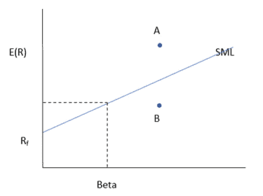
Likewise, there is Security Market Line (SML) that visually represents the Capital Asset Pricing Model (CAPM). The Security Market Line is represented by the following Eq. (4.7).
$$
S M L=\mathbf{r}{f}+\left[\beta *\left(\mathbf{r}{m}-\mathbf{r}_{f}\right)\right]
$$
The Security Market Line (SML) represents all the securities present in the market along with their corresponding $\beta$ values as shown in Fig. $4.5$.
The Security Market Line is often refereed by the market participants to decide whether an asset is priced correctly or not? According to the principle of Security Market Line, price of the asset labelled as $A$ is overpriced while asset $B$ is underpriced as shown in Fig. 4.5.
金融代写|金融计量经济学Financial Econometrics代考|Key Topics Covered
Asset pricing studies deal with the pricing of assets where assets can be debts, equity, bonds, derivatives, and others. In general, asset prices follow the law of demand and supply. The asset pricing studies have basically two schools of thought, namely theoretical and empirical. The former deals with the theoretical aspects of asset prices, whereas empirical asset pricing deals more with the quantitative characteristics. Empirical asset pricing deals with the real market data resulting more preferred by the market participants. Pricing of the debt instruments is considered to be much easier as compared to the equity pricing. Presence of various risk factors and uncertainty make asset pricing quite a challenging task. Markowitz (1952) modern portfolio theory laid the theoretical foundation for analysing the risk and return relationship. Thereafter Sharpe (1964) developed a single factor asset pricing model often referred as the capital asset pricing model (CAPM). According to the CAPM, cross section of the asset returns depends only on the cross section of the asset $\beta$ s. Since then over 300 different risk factors have been identified by the various studies, resulting in several multifactor asset pricing models developing since the development of CAPM. Maiti $(2020 \mathrm{a})$ highlighted that the evolution process of risk factors and factor models seems to be an endless development. Several risk factors that drive the asset prices are continuously changing and evolving over time. In addition to that still numerous risk factors are yet to be identified. All of these safe bets jointly make asset pricing a topic of somewhat more than that of the class room coaching.
The capital asset pricing model (CAPM) is the primary successful formal model of market equilibrium. CAPM fundamentally describes the relationship between the expected returns and systematic risk for financial assets. Similarly, the consumption-based capital asset pricing model (CCAPM) uses consumption beta instead of the market beta. The capital asset pricing model (CAPM) is represented by the below Eq. 5.1:
$$
E\left(r_{i}\right)=r_{f}+\beta *\left(r_{m}-r_{f}\right)
$$
where
$E\left(\mathrm{r}{i}\right)$ represent expected return of the assets $\mathrm{r}{f}$ is risk free rate of return
$\mathrm{r}_{m}$ is market return
$\beta$ measures return volatility
金融代写|金融计量经济学Financial Econometrics代考|What Is So Special About Fama and French
Fama and French estimated risk factors using the mimicking portfolio approach. The risk factors are estimated directly from the crosssectional asset returns sorted by the firm characteristics. Fama and French constructed their mimicking portfolios by using the single and double sorting techniques as shown in Table 5.1. Fama and French ranked the sample stocks every year in the month of June based on their market capitalization $(\mathrm{MC})$ and formed two portfolios, namely Big(B) and Small(S) using the NYSE median market cap breakpoint. Similarly,
three $\mathrm{BE} / \mathrm{ME}$ weighted portfolios, namely High(H), Neutral $(\mathrm{M})$, and Low(L), are constructed using the $30: 40: 30$ breakpoint. Then using the double sorting technique six portfolios are formed, namely $S / L, S / M$, $\mathrm{S} / \mathrm{H}, \mathrm{B} / \mathrm{L}, \mathrm{B} / \mathrm{M}$, and $\mathrm{B} / \mathrm{H}$. Portfolio $(\mathrm{S} / \mathrm{L})$ consists of the small $\mathrm{MC}$ stocks and low value $\mathrm{BE} / \mathrm{ME}$ stocks, whereas $(\mathrm{B} / \mathrm{H})$ consists of the big $M C$ stocks and high value $\mathrm{BE} / \mathrm{ME}$ stocks. The revision of portfolio formation is done every next year, and this process of portfolio revision continues till the end year.
SMB stands for the “small minus big” and represents risk mimicking portfolio for the size factor. Similarly, HML represents risk mimicking portfolio for the value factor. SMB and HML risk mimicking portfolios are estimated using the Eqs. $5.5$ and $5.6$.
$$
\begin{gathered}
\mathrm{SMB}=(S / L+S / M+S / H) / 3-(B / L+B / M+B / H) / 3 \
\mathrm{HML}=(S / H+B / H) / 2-(S / L+B / L) / 2
\end{gathered}
$$
Subsequently, other notable multifactor asset pricing models that developed are shown below in equation numbers from $5.7$ to $5.9$ :
Carhart (1997) four factor model (additional factor added is Momentum)
$$
\begin{aligned}
E\left(r_{i}\right)=& r_{f}+\beta_{i m} *\left(r_{m}-r_{f}\right)+\beta_{i s m b} *(\mathrm{SMB}) \
&+\beta_{i h m l} *(\mathrm{HML})+\beta_{i w m l} *(\mathrm{WML})+\varepsilon_{i}
\end{aligned}
$$
where WML is the Momentum factor
Fama and French (2015) five factor model (additional factor added are investment and profitability)
$$
\begin{aligned}
E\left(r_{i}\right)=& r_{f}+\beta_{i m} *\left(r_{m}-r_{f}\right)+\beta_{i s m b} *(\mathrm{SMB})+\beta_{i h m l} *(\mathrm{HML}) \
&+\beta_{i c m a} *(\mathrm{CMA})+\beta_{i r m w} *(\mathrm{RMW})+\varepsilon_{i}
\end{aligned}
$$
where CMA and RMW are the investment and profitability factors
$$
\begin{gathered}
\mathrm{CMA}=(S / C+B / C) / 2-(S / A+B / A) / 2 \
\mathrm{RMW}=(S / R+B / R) / 2-(S / W+B / W) / 2
\end{gathered}
$$
金融计量经济学代考
金融代写|金融计量经济学Financial Econometrics代考|Capital Market Line and Mean Variance Efficient Frontier
同样,平均方差有效边界,资本市场线 (CML) 是最佳组合风险和回报的所有投资组合的图形表示。平均方差有效边界与资本市场线的基本区别在于资本市场线将风险资产与非风险资产结合在一起。
在图 4.4 中,细实线代表资本市场线。资本市场线是从无风险收益率(Y 轴)绘制的直线,它在该点切割平均方差有效边界(风险资产的组合)米(代表最优投资组合)如图 4.4 所示。因此,资本市场线的斜率代表市场组合的夏普比率。投资组合的风险随着沿 CML 的上升而增加,而投资组合的风险随着沿 CML 的下降而降低。资本市场线由以下等式表示。
和(磷r)=rF+[r米−rFσ米]∗σp
在哪里
和(磷r)代表预期的投资组合回报rF是无风险收益率
r米是市场回报σ米是市场标准差的度量σp是投资组合标准差的度量
[r米−rFσ米]是市场投资组合的夏普比率
同样,证券市场线 (SML) 直观地代表了资本资产定价模型 (CAPM)。证券市场线由以下等式表示。(4.7)。
小号米大号=rF+[b∗(r米−rF)]
证券市场线 (SML) 代表市场上存在的所有证券及其对应的b值如图所示。4.5.
市场参与者经常参考证券市场线来决定资产定价是否正确?根据证券市场线原则,标为的资产价格为一个资产定价过高乙如图 4.5 所示,价格偏低。
金融代写|金融计量经济学Financial Econometrics代考|Key Topics Covered
资产定价研究处理资产的定价,其中资产可以是债务、股权、债券、衍生品等。一般来说,资产价格遵循供求规律。资产定价研究基本上有两种思想流派,即理论的和实证的。前者处理资产价格的理论方面,而经验资产定价更多地处理数量特征。经验资产定价处理更受市场参与者青睐的真实市场数据。与股权定价相比,债务工具的定价被认为要容易得多。各种风险因素和不确定性的存在使资产定价成为一项颇具挑战性的任务。Markowitz (1952) 现代投资组合理论为分析风险收益关系奠定了理论基础。此后 Sharpe (1964) 开发了一种单因素资产定价模型,通常称为资本资产定价模型 (CAPM)。根据 CAPM,资产收益的横截面只取决于资产的横截面bs。从那时起,各种研究已经确定了 300 多种不同的风险因素,导致自 CAPM 发展以来开发了几种多因素资产定价模型。迈提(2020一个)强调风险因素和因素模型的演化过程似乎是一个永无止境的发展。推动资产价格的几个风险因素随着时间的推移不断变化和演变。除此之外,还有许多风险因素尚待确定。所有这些安全的赌注共同使资产定价成为一个比课堂辅导更多的话题。
资本资产定价模型(CAPM)是市场均衡的主要成功的形式模型。CAPM 从根本上描述了金融资产的预期收益和系统风险之间的关系。同样,基于消费的资本资产定价模型(CCAPM)使用消费贝塔而不是市场贝塔。资本资产定价模型 (CAPM) 由以下等式表示。5.1:
和(r一世)=rF+b∗(r米−rF)
在哪里
和(r一世)代表资产的预期回报rF是无风险收益率
r米是市场回报
b衡量回报波动率
金融代写|金融计量经济学Financial Econometrics代考|What Is So Special About Fama and French
Fama 和 French 使用模拟投资组合方法估计风险因素。风险因素直接从按公司特征分类的横截面资产收益估计。Fama 和 French 使用表 5.1 所示的单次和双重排序技术构建了他们的模仿组合。Fama 和 French 在每年 6 月份根据其市值对样本股票进行排名(米C)并使用 NYSE 中值市值断点形成了两个投资组合,即 Big(B) 和 Small(S)。相似地,
三乙和/米和加权投资组合,即高(H),中性(米)和 Low(L) 是使用30:40:30断点。然后使用双重排序技术形成六个投资组合,即小号/大号,小号/米, 小号/H,乙/大号,乙/米, 和乙/H. 文件夹(小号/大号)由小米C股票和低价值乙和/米和股票,而(乙/H)由大米C股票和高价值乙和/米和股票。投资组合形成的修订每年进行一次,投资组合修订的过程一直持续到年底。
SMB 代表“小减大”,代表规模因子的风险模拟投资组合。同样,HML 代表价值因子的风险模拟投资组合。SMB 和 HML 风险模拟投资组合使用方程式进行估计。5.5和5.6.
小号米乙=(小号/大号+小号/米+小号/H)/3−(乙/大号+乙/米+乙/H)/3 H米大号=(小号/H+乙/H)/2−(小号/大号+乙/大号)/2
随后,开发的其他值得注意的多因素资产定价模型如下面的等式数字所示5.7至5.9 :
Carhart (1997) 四因子模型(添加的附加因子是动量)
和(r一世)=rF+b一世米∗(r米−rF)+b一世s米b∗(小号米乙) +b一世H米l∗(H米大号)+b一世在米l∗(在米大号)+e一世
其中 WML 是动量因子
Fama 和 French (2015) 五因子模型(添加的附加因子是投资和盈利能力)
和(r一世)=rF+b一世米∗(r米−rF)+b一世s米b∗(小号米乙)+b一世H米l∗(H米大号) +b一世C米一个∗(C米一个)+b一世r米在∗(R米在)+e一世
其中 CMA 和 RMW 是投资和盈利因素
C米一个=(小号/C+乙/C)/2−(小号/一个+乙/一个)/2 R米在=(小号/R+乙/R)/2−(小号/在+乙/在)/2

统计代写请认准statistics-lab™. statistics-lab™为您的留学生涯保驾护航。
金融工程代写
金融工程是使用数学技术来解决金融问题。金融工程使用计算机科学、统计学、经济学和应用数学领域的工具和知识来解决当前的金融问题,以及设计新的和创新的金融产品。
非参数统计代写
非参数统计指的是一种统计方法,其中不假设数据来自于由少数参数决定的规定模型;这种模型的例子包括正态分布模型和线性回归模型。
广义线性模型代考
广义线性模型(GLM)归属统计学领域,是一种应用灵活的线性回归模型。该模型允许因变量的偏差分布有除了正态分布之外的其它分布。
术语 广义线性模型(GLM)通常是指给定连续和/或分类预测因素的连续响应变量的常规线性回归模型。它包括多元线性回归,以及方差分析和方差分析(仅含固定效应)。
有限元方法代写
有限元方法(FEM)是一种流行的方法,用于数值解决工程和数学建模中出现的微分方程。典型的问题领域包括结构分析、传热、流体流动、质量运输和电磁势等传统领域。
有限元是一种通用的数值方法,用于解决两个或三个空间变量的偏微分方程(即一些边界值问题)。为了解决一个问题,有限元将一个大系统细分为更小、更简单的部分,称为有限元。这是通过在空间维度上的特定空间离散化来实现的,它是通过构建对象的网格来实现的:用于求解的数值域,它有有限数量的点。边界值问题的有限元方法表述最终导致一个代数方程组。该方法在域上对未知函数进行逼近。[1] 然后将模拟这些有限元的简单方程组合成一个更大的方程系统,以模拟整个问题。然后,有限元通过变化微积分使相关的误差函数最小化来逼近一个解决方案。
tatistics-lab作为专业的留学生服务机构,多年来已为美国、英国、加拿大、澳洲等留学热门地的学生提供专业的学术服务,包括但不限于Essay代写,Assignment代写,Dissertation代写,Report代写,小组作业代写,Proposal代写,Paper代写,Presentation代写,计算机作业代写,论文修改和润色,网课代做,exam代考等等。写作范围涵盖高中,本科,研究生等海外留学全阶段,辐射金融,经济学,会计学,审计学,管理学等全球99%专业科目。写作团队既有专业英语母语作者,也有海外名校硕博留学生,每位写作老师都拥有过硬的语言能力,专业的学科背景和学术写作经验。我们承诺100%原创,100%专业,100%准时,100%满意。
随机分析代写
随机微积分是数学的一个分支,对随机过程进行操作。它允许为随机过程的积分定义一个关于随机过程的一致的积分理论。这个领域是由日本数学家伊藤清在第二次世界大战期间创建并开始的。
时间序列分析代写
随机过程,是依赖于参数的一组随机变量的全体,参数通常是时间。 随机变量是随机现象的数量表现,其时间序列是一组按照时间发生先后顺序进行排列的数据点序列。通常一组时间序列的时间间隔为一恒定值(如1秒,5分钟,12小时,7天,1年),因此时间序列可以作为离散时间数据进行分析处理。研究时间序列数据的意义在于现实中,往往需要研究某个事物其随时间发展变化的规律。这就需要通过研究该事物过去发展的历史记录,以得到其自身发展的规律。
回归分析代写
多元回归分析渐进(Multiple Regression Analysis Asymptotics)属于计量经济学领域,主要是一种数学上的统计分析方法,可以分析复杂情况下各影响因素的数学关系,在自然科学、社会和经济学等多个领域内应用广泛。
MATLAB代写
MATLAB 是一种用于技术计算的高性能语言。它将计算、可视化和编程集成在一个易于使用的环境中,其中问题和解决方案以熟悉的数学符号表示。典型用途包括:数学和计算算法开发建模、仿真和原型制作数据分析、探索和可视化科学和工程图形应用程序开发,包括图形用户界面构建MATLAB 是一个交互式系统,其基本数据元素是一个不需要维度的数组。这使您可以解决许多技术计算问题,尤其是那些具有矩阵和向量公式的问题,而只需用 C 或 Fortran 等标量非交互式语言编写程序所需的时间的一小部分。MATLAB 名称代表矩阵实验室。MATLAB 最初的编写目的是提供对由 LINPACK 和 EISPACK 项目开发的矩阵软件的轻松访问,这两个项目共同代表了矩阵计算软件的最新技术。MATLAB 经过多年的发展,得到了许多用户的投入。在大学环境中,它是数学、工程和科学入门和高级课程的标准教学工具。在工业领域,MATLAB 是高效研究、开发和分析的首选工具。MATLAB 具有一系列称为工具箱的特定于应用程序的解决方案。对于大多数 MATLAB 用户来说非常重要,工具箱允许您学习和应用专业技术。工具箱是 MATLAB 函数(M 文件)的综合集合,可扩展 MATLAB 环境以解决特定类别的问题。可用工具箱的领域包括信号处理、控制系统、神经网络、模糊逻辑、小波、仿真等。