标签: ECMT2130

金融代写|金融计量经济学代写Financial Econometrics代考|ECMT6006

如果你也在 怎样代写金融计量经济学Financial Econometrics这个学科遇到相关的难题,请随时右上角联系我们的24/7代写客服。

金融计量学是将统计方法应用于金融市场数据。金融计量学是金融经济学的一个分支,在经济学领域。研究领域包括资本市场、金融机构、公司财务和公司治理。

statistics-lab™ 为您的留学生涯保驾护航 在代写金融计量经济学Financial Econometrics方面已经树立了自己的口碑, 保证靠谱, 高质且原创的统计Statistics代写服务。我们的专家在代写金融计量经济学Financial Econometrics代写方面经验极为丰富,各种代写金融计量经济学Financial Econometrics相关的作业也就用不着说。

我们提供的金融计量经济学Financial Econometrics及其相关学科的代写,服务范围广, 其中包括但不限于:

  • Statistical Inference 统计推断
  • Statistical Computing 统计计算
  • Advanced Probability Theory 高等概率论
  • Advanced Mathematical Statistics 高等数理统计学
  • (Generalized) Linear Models 广义线性模型
  • Statistical Machine Learning 统计机器学习
  • Longitudinal Data Analysis 纵向数据分析
  • Foundations of Data Science 数据科学基础
金融代写|金融计量经济学代写Financial Econometrics代考|ECMT6006

金融代写|金融计量经济学Financial Econometrics代考|ARIMA

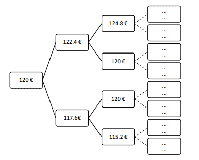
An important aspect of the time series is that time series data is often used for the forecasting. Based on the information of the past and present states of the variable, the future states of the variable are forecasted. The ARIMA models are introduced by the Box-Jenkins in the year 1976. The ARIMA stands for the “Auto Regressive Integrated Moving Average”. Thereafter, ARIMA models are widely used in finance for forecasting the stationary time series. The ARIMA models are useful for modelling both the univariate and multivariate time series. Commonly, time series is generated using the following: AR (Autoregressive) or MA (Moving average) or both (ARMA) or ARIMA processes.

AR (Autoregressive) Process
The AR (Autoregressive) process considers the past values of the time series for modelling. The first order AR (Autoregressive) model is represented by following Eq. $6.3$.
$$
R_{I}=\Phi_{l} R_{t-1}+\mathbf{u}{t} $$ Where $R{t}$ represents the present value of the variable at time $t$
$R_{t-1}$ represents the past value of the variable at time $t-1$
$\Phi_{t}$ represents the proportion at time $t$
$\mathrm{u}{t}$ represents the white noise error term The above Eq. (6.3) represents that the present value of the variable $(R)$ at time $(t)$ is equal to the some proportion $\left(\Phi{t}\right)$ of the past value of the variable $(R)$ at time $(t-1)$ plus the white noise error term $\left(\mathrm{u}{t}\right)$. Likewise, $\mathrm{nth}$ order AR (Autoregressive) process or $\mathrm{AR}(\mathrm{n})$ can be represented as Eq. (6.4). The $\mathrm{AR}(\mathrm{n})$ model as shown in $(6.4)$ includes only the current and previous values of the variable $R$. $$ R{t}=\Phi_{1} R_{t-1}+\Phi_{2} R_{t-2}+\ldots+\Phi_{n} R_{t-n}+\mathrm{u}_{t}
$$
Basic properties of the $\mathrm{AR}$ (Autoregressive) process are as follows:

  • Mean of the $R_{t}$ for $\mathrm{AR}$ (1) model is zero
  • Variance of $R_{t}$ for $\mathrm{AR}$ (1) model is represented by the Eq. (6.5)
    $$
    \frac{\sigma_{u}^{2}}{\left(1-\Phi_{1}^{2}\right)}
    $$
  • Covariance between $R_{t}$ and $R_{t-1}$ is represented by the Eq. (6.6)
    $$
    \frac{\Phi_{1} \sigma_{u}^{2}}{\left(1-\Phi_{1}^{2}\right)}
    $$
    Similarly for lag $(\mathrm{n})$ the expression is shown below
    $$
    \frac{\Phi_{1}^{n} \sigma_{u}^{2}}{\left(1-\Phi_{1}^{2}\right)}
    $$

金融代写|金融计量经济学Financial Econometrics代考|ARCH & GARCH

The ARMA models are good in explaining the serial correlation but not efficient in capturing the conditional heteroskedasticity or volatility clustering. Thus, for forecasting the time series accurately, there is need for more sophisticated techniques. The ARCH (see Engle, 1982, 1983) and GARCH (see Bollerslev, 1986) techniques are used widely for modelling the volatility or volatility clustering of the time series. An ARCH model can be estimated from the best fitting autoregressive (AR) model using the OLS. Then perform the ARCH test to check whether ARCH effect is present in the residuals obtained from the autoregressive (AR) regression. The best fitting autoregressive (AR) model can be represented by the Eq. (6.13).

$$
Y_{I}=\alpha_{0}+\alpha_{1} Y_{t-1}+\alpha_{2} Y_{t-2}+\ldots+\alpha_{n} Y_{t-n}+\mathrm{u}{t} $$ Next, estimate the squares of the error term $\left(\hat{\mathrm{u}}{t}^{2}\right) \hat{\epsilon}^{2}$ by running a regression on the lagged value of the squares of the error term $\left(\hat{\mathrm{u}}{t}^{2}\right) \hat{\epsilon}^{2}$. $$ \hat{\mathbf{u}}{t}^{2}=\alpha_{0}+\sum_{i=1}^{p} \alpha_{i} \hat{\mathbf{u}}{t-i}^{2} u $$ In the above Eq. (6.14), $p$ represents the length of The ARCH lags. The null hypothesis of the $\mathrm{ARCH}$ test assumes that there is no $\mathrm{ARCH}$ effect present in the time series. The GARCH model considers the lagged conditional variance term in addition to the lagged value of the squares of the error term $\hat{\epsilon}^{2}$. The generalized GARCH $(p, q)$ model can be represented mathematically as shown in the Eq. (6.15). $$ \hat{\mathrm{u}}{t}^{2}=\alpha_{0}+\sum_{i=1}^{p} \alpha_{i} \hat{\mathrm{u}}{t-i}^{2}+\sum{i=1}^{q} \beta_{i} \sigma_{t-i}^{2}
$$
Where
P represents the lags length of the lagged value of the squares of the error term $\hat{\epsilon}^{2}$
$Q$ represents the lags length of the lagged conditional variance terms.

金融代写|金融计量经济学Financial Econometrics代考|VAR

The VAR stands for the “Vector Autoregressive”. The VAR models are introduced by Christopher A. Sim in the year 1960. VAR models are useful specially on dealing with the multivariate time series over time. The VAR model structure of a variable includes linear function of the lagged values of the variable and all other variables included in the VAR model. Let’s characterize a VAR model for examining the variations in the $\mathrm{X}$ and $\mathrm{Y}$ variables. Mathematically, the above VAR model can be represented as Eq. (6.16 and 6.17).
$$
\begin{aligned}
&X_{t}=\alpha_{1}+\sum_{i=1}^{p} \beta_{i} X_{t-i}+\sum_{i=1}^{p} \gamma_{i} Y_{t-i}+\mathrm{u}{1 t} \ &Y{t}=\alpha_{2}+\sum_{i=1}^{p} \theta_{i} X_{t-i}+\sum_{i=1}^{p} \lambda_{i} Y_{t-i}+\mathrm{u}_{2 t}
\end{aligned}
$$ The above two Eqs. (6.16 and 6.17) represent the VAR $(p)$ model. Where, $p$ represents the length of the lags. The VAR models assume that the variables are stationary. However, if the variables are not stationary but cointegrated, then VECM (Vector Error Correction Model) may be useful. The regression analysis expresses the dependency of one variable on the other. But it does not express the causality among the variables. The Granger Causality Test estimates provide detailed information on the causality among the variables. The VAR models are likewise useful to estimate the impulse response analysis and variance decomposition.

金融代写|金融计量经济学代写Financial Econometrics代考|ECMT6006

金融计量经济学代考

金融代写|金融计量经济学Financial Econometrics代考|ARIMA

时间序列的一个重要方面是时间序列数据通常用于预测。根据变量过去和现在的状态信息,预测变量的未来状态。ARIMA 模型由 Box-Jenkins 在 1976 年推出。ARIMA 代表“自动回归综合移动平均线”。此后,ARIMA 模型在金融领域广泛用于预测平稳时间序列。ARIMA 模型可用于对单变量和多变量时间序列进行建模。通常,使用以下方法生成时间序列:AR(自回归)或 MA(移动平均)或两者(ARMA)或 ARIMA 过程。

AR(自回归)过程
AR(自回归)过程考虑时间序列的过去值进行建模。一阶 AR(自回归)模型由以下等式表示。6.3.

R我=披lR吨−1+在吨在哪里R吨表示变量在时间的现值吨
R吨−1表示变量在某个时间的过去值吨−1
披吨表示当时的比例吨
在吨表示白噪声误差项 (6.3) 表示变量的现值(R)有时(吨)等于某个比例(披吨)变量的过去值(R)有时(吨−1)加上白噪声误差项(在吨). 同样地,n吨H订购 AR(自回归)过程或一个R(n)可以表示为等式。(6.4)。这一个R(n)模型如图所示(6.4)仅包括变量的当前值和先前值R.

R吨=披1R吨−1+披2R吨−2+…+披nR吨−n+在吨
基本属性一个R(自回归)过程如下:

  • 的平均值R吨为了一个R(1) 模型为零
  • 方差R吨为了一个R(1) 模型由方程式表示。(6.5)
    σ在2(1−披12)
  • 之间的协方差R吨和R吨−1由方程式表示。(6.6)
    披1σ在2(1−披12)
    同样对于滞后(n)表达式如下所示
    披1nσ在2(1−披12)

金融代写|金融计量经济学Financial Econometrics代考|ARCH & GARCH

ARMA 模型能很好地解释序列相关性,但不能有效地捕捉条件异方差或波动率聚类。因此,为了准确地预测时间序列,需要更复杂的技术。ARCH(参见 Engle, 1982, 1983)和 GARCH(参见 Bollerslev, 1986)技术被广泛用于时间序列的波动率或波动率聚类建模。可以使用 OLS 从最佳拟合自回归 (AR) 模型估计 ARCH 模型。然后执行 ARCH 测试以检查从自回归 (AR) 回归获得的残差中是否存在 ARCH 效应。最佳拟合自回归 (AR) 模型可以由方程式表示。(6.13)。

是我=一个0+一个1是吨−1+一个2是吨−2+…+一个n是吨−n+在吨接下来,估计误差项的平方(在^吨2)ε^2通过对误差项平方的滞后值进行回归(在^吨2)ε^2.

在^吨2=一个0+∑一世=1p一个一世在^吨−一世2在在上面的方程式中。(6.14),p表示 ARCH 滞后的长度。的零假设一个RCH测试假设没有一个RCH时间序列中存在的影响。GARCH 模型除了误差项平方的滞后值外,还考虑滞后条件方差项ε^2. 广义 GARCH(p,q)模型可以用数学方式表示,如方程式所示。(6.15)。

在^吨2=一个0+∑一世=1p一个一世在^吨−一世2+∑一世=1qb一世σ吨−一世2
其中
P 表示误差项平方的滞后值的滞后长度ε^2
问表示滞后条件方差项的滞后长度。

金融代写|金融计量经济学Financial Econometrics代考|VAR

VAR 代表“向量自回归”。VAR 模型由 Christopher A. Sim 在 1960 年引入。VAR 模型特别适用于处理随时间变化的多元时间序列。变量的 VAR 模型结构包括变量滞后值和 VAR 模型中包含的所有其他变量的线性函数。让我们描述一个 VAR 模型来检查X和是变量。在数学上,上述 VAR 模型可以表示为等式。(6.16 和 6.17)。
$$
\begin{aligned}
&X_{t}=\alpha_{1}+\sum_{i=1}^{p} \beta_{i} X_{ti}+\sum_{i=1}^{p} \gamma_{i} Y_{ti}+\mathrm{u} {1 t} \ &Y {t}=\alpha_{2}+\sum_{i=1}^{p} \theta_{i} X_{ti }+\sum_{i=1}^{p} \lambda_{i} Y_{ti}+\mathrm{u}_{2 t}
\end{aligned}
$$ 以上两个方程。(6.16 和 6.17) 代表 VAR(p)模型。在哪里,p表示滞后的长度。VAR 模型假设变量是平稳的。但是,如果变量不是平稳的而是协整的,那么 VECM(矢量误差校正模型)可能会很有用。回归分析表达了一个变量对另一个变量的依赖性。但它并没有表达变量之间的因果关系。格兰杰因果检验估计提供了变量间因果关系的详细信息。VAR 模型同样可用于估计脉冲响应分析和方差分解。

金融代写|金融计量经济学Financial Econometrics代考 请认准statistics-lab™

统计代写请认准statistics-lab™. statistics-lab™为您的留学生涯保驾护航。

金融工程代写

金融工程是使用数学技术来解决金融问题。金融工程使用计算机科学、统计学、经济学和应用数学领域的工具和知识来解决当前的金融问题,以及设计新的和创新的金融产品。

非参数统计代写

非参数统计指的是一种统计方法,其中不假设数据来自于由少数参数决定的规定模型;这种模型的例子包括正态分布模型和线性回归模型。

广义线性模型代考

广义线性模型(GLM)归属统计学领域,是一种应用灵活的线性回归模型。该模型允许因变量的偏差分布有除了正态分布之外的其它分布。

术语 广义线性模型(GLM)通常是指给定连续和/或分类预测因素的连续响应变量的常规线性回归模型。它包括多元线性回归,以及方差分析和方差分析(仅含固定效应)。

有限元方法代写

有限元方法(FEM)是一种流行的方法,用于数值解决工程和数学建模中出现的微分方程。典型的问题领域包括结构分析、传热、流体流动、质量运输和电磁势等传统领域。

有限元是一种通用的数值方法,用于解决两个或三个空间变量的偏微分方程(即一些边界值问题)。为了解决一个问题,有限元将一个大系统细分为更小、更简单的部分,称为有限元。这是通过在空间维度上的特定空间离散化来实现的,它是通过构建对象的网格来实现的:用于求解的数值域,它有有限数量的点。边界值问题的有限元方法表述最终导致一个代数方程组。该方法在域上对未知函数进行逼近。[1] 然后将模拟这些有限元的简单方程组合成一个更大的方程系统,以模拟整个问题。然后,有限元通过变化微积分使相关的误差函数最小化来逼近一个解决方案。

tatistics-lab作为专业的留学生服务机构,多年来已为美国、英国、加拿大、澳洲等留学热门地的学生提供专业的学术服务,包括但不限于Essay代写,Assignment代写,Dissertation代写,Report代写,小组作业代写,Proposal代写,Paper代写,Presentation代写,计算机作业代写,论文修改和润色,网课代做,exam代考等等。写作范围涵盖高中,本科,研究生等海外留学全阶段,辐射金融,经济学,会计学,审计学,管理学等全球99%专业科目。写作团队既有专业英语母语作者,也有海外名校硕博留学生,每位写作老师都拥有过硬的语言能力,专业的学科背景和学术写作经验。我们承诺100%原创,100%专业,100%准时,100%满意。

随机分析代写


随机微积分是数学的一个分支,对随机过程进行操作。它允许为随机过程的积分定义一个关于随机过程的一致的积分理论。这个领域是由日本数学家伊藤清在第二次世界大战期间创建并开始的。

时间序列分析代写

随机过程,是依赖于参数的一组随机变量的全体,参数通常是时间。 随机变量是随机现象的数量表现,其时间序列是一组按照时间发生先后顺序进行排列的数据点序列。通常一组时间序列的时间间隔为一恒定值(如1秒,5分钟,12小时,7天,1年),因此时间序列可以作为离散时间数据进行分析处理。研究时间序列数据的意义在于现实中,往往需要研究某个事物其随时间发展变化的规律。这就需要通过研究该事物过去发展的历史记录,以得到其自身发展的规律。

回归分析代写

多元回归分析渐进(Multiple Regression Analysis Asymptotics)属于计量经济学领域,主要是一种数学上的统计分析方法,可以分析复杂情况下各影响因素的数学关系,在自然科学、社会和经济学等多个领域内应用广泛。

MATLAB代写

MATLAB 是一种用于技术计算的高性能语言。它将计算、可视化和编程集成在一个易于使用的环境中,其中问题和解决方案以熟悉的数学符号表示。典型用途包括:数学和计算算法开发建模、仿真和原型制作数据分析、探索和可视化科学和工程图形应用程序开发,包括图形用户界面构建MATLAB 是一个交互式系统,其基本数据元素是一个不需要维度的数组。这使您可以解决许多技术计算问题,尤其是那些具有矩阵和向量公式的问题,而只需用 C 或 Fortran 等标量非交互式语言编写程序所需的时间的一小部分。MATLAB 名称代表矩阵实验室。MATLAB 最初的编写目的是提供对由 LINPACK 和 EISPACK 项目开发的矩阵软件的轻松访问,这两个项目共同代表了矩阵计算软件的最新技术。MATLAB 经过多年的发展,得到了许多用户的投入。在大学环境中,它是数学、工程和科学入门和高级课程的标准教学工具。在工业领域,MATLAB 是高效研究、开发和分析的首选工具。MATLAB 具有一系列称为工具箱的特定于应用程序的解决方案。对于大多数 MATLAB 用户来说非常重要,工具箱允许您学习应用专业技术。工具箱是 MATLAB 函数(M 文件)的综合集合,可扩展 MATLAB 环境以解决特定类别的问题。可用工具箱的领域包括信号处理、控制系统、神经网络、模糊逻辑、小波、仿真等。

R语言代写问卷设计与分析代写
PYTHON代写回归分析与线性模型代写
MATLAB代写方差分析与试验设计代写
STATA代写机器学习/统计学习代写
SPSS代写计量经济学代写
EVIEWS代写时间序列分析代写
EXCEL代写深度学习代写
SQL代写各种数据建模与可视化代写

金融代写|金融计量经济学代写Financial Econometrics代考|ECMT2130

如果你也在 怎样代写金融计量经济学Financial Econometrics这个学科遇到相关的难题,请随时右上角联系我们的24/7代写客服。

金融计量学是将统计方法应用于金融市场数据。金融计量学是金融经济学的一个分支,在经济学领域。研究领域包括资本市场、金融机构、公司财务和公司治理。

statistics-lab™ 为您的留学生涯保驾护航 在代写金融计量经济学Financial Econometrics方面已经树立了自己的口碑, 保证靠谱, 高质且原创的统计Statistics代写服务。我们的专家在代写金融计量经济学Financial Econometrics代写方面经验极为丰富,各种代写金融计量经济学Financial Econometrics相关的作业也就用不着说。

我们提供的金融计量经济学Financial Econometrics及其相关学科的代写,服务范围广, 其中包括但不限于:

  • Statistical Inference 统计推断
  • Statistical Computing 统计计算
  • Advanced Probability Theory 高等概率论
  • Advanced Mathematical Statistics 高等数理统计学
  • (Generalized) Linear Models 广义线性模型
  • Statistical Machine Learning 统计机器学习
  • Longitudinal Data Analysis 纵向数据分析
  • Foundations of Data Science 数据科学基础
金融代写|金融计量经济学代写Financial Econometrics代考|ECMT2130

金融代写|金融计量经济学Financial Econometrics代考|Real-World Tasks

A professor asks his/her student to test CAPM in Australian context. Assume yourself as the student and perform the task. Then prepare a detailed report of the analysis to be submitted to the professor.

  1. A researcher want to test the performance of the CAPM and APT models in crypto markets. Assume yourself as the researcher: perform the mentioned task in detail and develop the analysis report.
  2. An analyst is currently evaluating an investment option to invest in the major global currencies. To do so he/she want to test the APT model for making the investment decision. Help him/her to perform the said analysis and prepare the report.
  3. A student needs to identify whether there exists size and value patterns in the BSE 500 securities mean excess returns. Help the student to complete his/her project dissertation successfully and satisfactorily.
  4. An assistant manager of the Reserve Bank of New Zealand asked a junior working under him/her to prepare a detailed report on “How efficient is Fama and French multifactor models in Australia and New Zealand”? Help the junior in developing the final report for timely submission to the assistant manager of Reserve Bank of New Zealand.
  5. There is a disagreement between two market participants that “the CCAPM isn’t Perfect”. So they approach to an expert to clarify it? Assume yourself as that expert and advise them on it with appropriate examples.
  6. A researcher want to examine whether financial leverage is an important firm specific factor specially in the emerging markets? The researcher is also interested to check whether financial leverage alone or financial leverage along with other firm specific factors can capture risk-return relationship better. Help the researcher to conduct and complete the analysis satisfactorily.

金融代写|金融计量经济学Financial Econometrics代考|Case Studies

To examine the performance of CAPM and Fama-French three factor models in Sri Lankan context. The regressions and GRS test are implemented to examine the asset pricing models performance. The obtained regressions and GRS test estimates are shown below. Based on these obtained estimates comment on the performance of these two asset pricing models.

Data Description:
Colombo Stock Exchange traded securities are used to construct the study portfolios based on the size (market capitalization) and value ( $\mathrm{P} / \mathrm{B}$ ratio) factors by means of the Fama-French (1993) technique. For risk free rate Sri Lankan government 10 years bond are used. S\&P 20 index mean excess returns used as proxy for the market. The study period is between July 2008 and May 2016. All data points are in monthly frequency.
Regression models used are as follows:
CAPM or Fama-French Three Factor Model
$$
E\left(r_{i}\right)-r_{f}=\alpha_{i}+\beta_{i m} *\left(r_{m}-r_{f}\right)+\varepsilon_{i}
$$
$$
E\left(r_{i}\right)-r_{f}=\alpha_{i}+\beta_{i m} *\left(r_{m}-r_{f}\right)+\beta_{i s} *(\text { Size })+\beta_{i v} *(\text { Value })+\varepsilon_{i}
$$
Estimates:
CAPM regression estimates for 25 portfolios based on size and value factors.

金融代写|金融计量经济学Financial Econometrics代考|Risk Analysis

Risk analysis is the heart of any financial decision-making process. Time series of a variable consists of the data points over time. Time series data of a variable comprises several important information about the variable over time. Original time series data can be decomposed into various components, namely seasonal, trend, and remainder components. Time series can be easily decomposed into its various components by using the STL (Seasonal and Trend decomposition using LOESS) decomposition technique as suggested by Cleveland et al. (1990). The LOESS is a robust technique and its abbreviation stands for the “locally estimated scatter” plot smoothing”. The LOESS is a non-parametric technique used for the smooth curve fitting. The STL decomposes the time series into different components using an additive function as shown below in Eq. 6.1.
$$
\text { Timeseries }=\text { Trend }+\text { Seasonal }+\text { Remainder }
$$
The STL technique has certain limitations such as it is not efficient enough in handling the trading day or calendar variation automatically. This above limitation can be overcome by using a multiplicative decomposition function as defined in Eq. $6.2$.
$$
\text { Timeseries }=\text { Trend } * \text { Seasonal } * \text { Remainder }
$$
Thus to analyse the time series, a good knowledge of the essential time series econometrics methods are necessary. The time series econometrics deal with the measurement of the random variables over time. The time series analysis is useful for determining how a variable changes over time. It is also equally important in assessing the impact of the other factors on the study variable over the same time frame. The paragraphs below covered all such essential time series econometrics techniques to deal with the time series data.

金融代写|金融计量经济学代写Financial Econometrics代考|ECMT2130

金融计量经济学代考

金融代写|金融计量经济学Financial Econometrics代考|Real-World Tasks

一位教授要求他/她的学生在澳大利亚环境中测试 CAPM。假设自己是学生并执行任务。然后准备一份详细的分析报告提交给教授。

  1. 一位研究人员想要测试 CAPM 和 APT 模型在加密市场中的性能。假设自己是研究人员:详细执行上述任务并制定分析报告。
  2. 一位分析师目前正在评估一种投资全球主要货币的投资选择。为此,他/她想测试 APT 模型以做出投资决策。帮助他/她进行上述分析并准备报告。
  3. 学生需要确定 BSE 500 证券平均超额收益中是否存在规模和价值模式。帮助学生成功并令人满意地完成他/她的项目论文。
  4. 新西兰储备银行的一位助理经理让他/她手下的一名初级工作人员准备一份关于“Fama 和 French 多因素模型在澳大利亚和新西兰的效率如何”的详细报告?帮助小学生制定最终报告,以便及时提交给新西兰储备银行的助理经理。
  5. 两个市场参与者之间存在分歧,即“CCAPM 并不完美”。所以他们找专家来澄清一下?假设你自己是那个专家,并用适当的例子给他们建议。
  6. 研究人员想检查财务杠杆是否是一个重要的公司特定因素,特别是在新兴市场?研究人员也有兴趣检查单独的财务杠杆或财务杠杆与其他公司特定因素是否可以更好地捕捉风险回报关系。帮助研究人员令人满意地进行和完成分析。

金融代写|金融计量经济学Financial Econometrics代考|Case Studies

检验 CAPM 和 Fama-French 三因子模型在斯里兰卡背景下的表现。实施回归和 GRS 测试以检查资产定价模型的性能。获得的回归和 GRS 测试估计如下所示。基于这些获得的估计,对这两种资产定价模型的表现进行评论。

数据说明:
科伦坡证券交易所交易证券用于根据规模(市值)和价值(磷/乙比率)因子通过 Fama-French (1993) 技术。对于无风险利率,使用斯里兰卡政府 10 年期债券。标准普尔 20 指数的平均超额收益用作市场的代表。研究期为 2008 年 7 月至 2016 年 5 月。所有数据点均按月计算。
使用的回归模型如下:
CAPM 或 Fama-French 三因素模型

和(r一世)−rF=一个一世+b一世米∗(r米−rF)+e一世

和(r一世)−rF=一个一世+b一世米∗(r米−rF)+b一世s∗( 尺寸 )+b一世在∗( 价值 )+e一世
估计:
基于规模和价值因素的 25 个投资组合的 CAPM 回归估计。

金融代写|金融计量经济学Financial Econometrics代考|Risk Analysis

风险分析是任何财务决策过程的核心。变量的时间序列由随时间变化的数据点组成。变量的时间序列数据包含有关该变量随时间变化的几个重要信息。原始时间序列数据可以分解为各种成分,即季节性成分、趋势成分和剩余成分。通过使用 Cleveland 等人建议的 STL(使用 LOESS 的季节和趋势分解)分解技术,时间序列可以很容易地分解为其各个组成部分。(1990)。LOESS 是一种稳健的技术,其缩写代表“局部估计散点图平滑”。LOESS 是一种用于平滑曲线拟合的非参数技术。STL 使用加法函数将时间序列分解为不同的分量,如下面的方程式所示。6.1。

 时间序列 = 趋势 + 季节性 + 余 
STL 技术有一定的局限性,例如在自动处理交易日或日历变化方面效率不够。可以通过使用方程式中定义的乘法分解函数来克服上述限制。6.2.

 时间序列 = 趋势 ∗ 季节性 ∗ 余 
因此,要分析时间序列,需要对基本的时间序列计量经济学方法有很好的了解。时间序列计量经济学处理随时间变化的随机变量的测量。时间序列分析可用于确定变量如何随时间变化。在评估同一时间框架内其他因素对研究变量的影响方面也同样重要。以下段落涵盖了处理时间序列数据的所有这些基本时间序列计量经济学技术。

金融代写|金融计量经济学Financial Econometrics代考 请认准statistics-lab™

统计代写请认准statistics-lab™. statistics-lab™为您的留学生涯保驾护航。

金融工程代写

金融工程是使用数学技术来解决金融问题。金融工程使用计算机科学、统计学、经济学和应用数学领域的工具和知识来解决当前的金融问题,以及设计新的和创新的金融产品。

非参数统计代写

非参数统计指的是一种统计方法,其中不假设数据来自于由少数参数决定的规定模型;这种模型的例子包括正态分布模型和线性回归模型。

广义线性模型代考

广义线性模型(GLM)归属统计学领域,是一种应用灵活的线性回归模型。该模型允许因变量的偏差分布有除了正态分布之外的其它分布。

术语 广义线性模型(GLM)通常是指给定连续和/或分类预测因素的连续响应变量的常规线性回归模型。它包括多元线性回归,以及方差分析和方差分析(仅含固定效应)。

有限元方法代写

有限元方法(FEM)是一种流行的方法,用于数值解决工程和数学建模中出现的微分方程。典型的问题领域包括结构分析、传热、流体流动、质量运输和电磁势等传统领域。

有限元是一种通用的数值方法,用于解决两个或三个空间变量的偏微分方程(即一些边界值问题)。为了解决一个问题,有限元将一个大系统细分为更小、更简单的部分,称为有限元。这是通过在空间维度上的特定空间离散化来实现的,它是通过构建对象的网格来实现的:用于求解的数值域,它有有限数量的点。边界值问题的有限元方法表述最终导致一个代数方程组。该方法在域上对未知函数进行逼近。[1] 然后将模拟这些有限元的简单方程组合成一个更大的方程系统,以模拟整个问题。然后,有限元通过变化微积分使相关的误差函数最小化来逼近一个解决方案。

tatistics-lab作为专业的留学生服务机构,多年来已为美国、英国、加拿大、澳洲等留学热门地的学生提供专业的学术服务,包括但不限于Essay代写,Assignment代写,Dissertation代写,Report代写,小组作业代写,Proposal代写,Paper代写,Presentation代写,计算机作业代写,论文修改和润色,网课代做,exam代考等等。写作范围涵盖高中,本科,研究生等海外留学全阶段,辐射金融,经济学,会计学,审计学,管理学等全球99%专业科目。写作团队既有专业英语母语作者,也有海外名校硕博留学生,每位写作老师都拥有过硬的语言能力,专业的学科背景和学术写作经验。我们承诺100%原创,100%专业,100%准时,100%满意。

随机分析代写


随机微积分是数学的一个分支,对随机过程进行操作。它允许为随机过程的积分定义一个关于随机过程的一致的积分理论。这个领域是由日本数学家伊藤清在第二次世界大战期间创建并开始的。

时间序列分析代写

随机过程,是依赖于参数的一组随机变量的全体,参数通常是时间。 随机变量是随机现象的数量表现,其时间序列是一组按照时间发生先后顺序进行排列的数据点序列。通常一组时间序列的时间间隔为一恒定值(如1秒,5分钟,12小时,7天,1年),因此时间序列可以作为离散时间数据进行分析处理。研究时间序列数据的意义在于现实中,往往需要研究某个事物其随时间发展变化的规律。这就需要通过研究该事物过去发展的历史记录,以得到其自身发展的规律。

回归分析代写

多元回归分析渐进(Multiple Regression Analysis Asymptotics)属于计量经济学领域,主要是一种数学上的统计分析方法,可以分析复杂情况下各影响因素的数学关系,在自然科学、社会和经济学等多个领域内应用广泛。

MATLAB代写

MATLAB 是一种用于技术计算的高性能语言。它将计算、可视化和编程集成在一个易于使用的环境中,其中问题和解决方案以熟悉的数学符号表示。典型用途包括:数学和计算算法开发建模、仿真和原型制作数据分析、探索和可视化科学和工程图形应用程序开发,包括图形用户界面构建MATLAB 是一个交互式系统,其基本数据元素是一个不需要维度的数组。这使您可以解决许多技术计算问题,尤其是那些具有矩阵和向量公式的问题,而只需用 C 或 Fortran 等标量非交互式语言编写程序所需的时间的一小部分。MATLAB 名称代表矩阵实验室。MATLAB 最初的编写目的是提供对由 LINPACK 和 EISPACK 项目开发的矩阵软件的轻松访问,这两个项目共同代表了矩阵计算软件的最新技术。MATLAB 经过多年的发展,得到了许多用户的投入。在大学环境中,它是数学、工程和科学入门和高级课程的标准教学工具。在工业领域,MATLAB 是高效研究、开发和分析的首选工具。MATLAB 具有一系列称为工具箱的特定于应用程序的解决方案。对于大多数 MATLAB 用户来说非常重要,工具箱允许您学习应用专业技术。工具箱是 MATLAB 函数(M 文件)的综合集合,可扩展 MATLAB 环境以解决特定类别的问题。可用工具箱的领域包括信号处理、控制系统、神经网络、模糊逻辑、小波、仿真等。

R语言代写问卷设计与分析代写
PYTHON代写回归分析与线性模型代写
MATLAB代写方差分析与试验设计代写
STATA代写机器学习/统计学习代写
SPSS代写计量经济学代写
EVIEWS代写时间序列分析代写
EXCEL代写深度学习代写
SQL代写各种数据建模与可视化代写

金融代写|金融计量经济学代写Financial Econometrics代考|ECOM90011

如果你也在 怎样代写金融计量经济学Financial Econometrics这个学科遇到相关的难题,请随时右上角联系我们的24/7代写客服。

金融计量学是将统计方法应用于金融市场数据。金融计量学是金融经济学的一个分支,在经济学领域。研究领域包括资本市场、金融机构、公司财务和公司治理。

statistics-lab™ 为您的留学生涯保驾护航 在代写金融计量经济学Financial Econometrics方面已经树立了自己的口碑, 保证靠谱, 高质且原创的统计Statistics代写服务。我们的专家在代写金融计量经济学Financial Econometrics代写方面经验极为丰富,各种代写金融计量经济学Financial Econometrics相关的作业也就用不着说。

我们提供的金融计量经济学Financial Econometrics及其相关学科的代写,服务范围广, 其中包括但不限于:

  • Statistical Inference 统计推断
  • Statistical Computing 统计计算
  • Advanced Probability Theory 高等概率论
  • Advanced Mathematical Statistics 高等数理统计学
  • (Generalized) Linear Models 广义线性模型
  • Statistical Machine Learning 统计机器学习
  • Longitudinal Data Analysis 纵向数据分析
  • Foundations of Data Science 数据科学基础
金融代写|金融计量经济学代写Financial Econometrics代考|ECOM90011

金融代写|金融计量经济学Financial Econometrics代考|How to Test One Model Versus the Other

Testing one model versus the other model is vital in asset pricing studies. All of the available notable asset pricing models are not absolutely accurate. It is also true that if there is not enough data then any asset pricing model can be easily rejected by the standard tests. Every so often it is tacit that in the data which model is the better model than some other model? To do so numerous statistical inferences are used.

Let’s consider the Fama and French five factor model as shown in Eq. $5.8 .$
$$
\begin{aligned}
E\left(r_{i}\right)=& r_{f}+\beta_{i m} *\left(r_{m}-r_{f}\right)+\beta_{i s m b} *(\mathrm{SMB})+\beta_{i h m l} *(\mathrm{HML}) \
&+\beta_{i c m a} *(\mathrm{CMA})+\beta_{i r m w} *(\mathrm{RMW})+\varepsilon_{i}
\end{aligned}
$$

Can a factor be dropped from the above model?
For instance, consider the HML factor dropped from the above model. How to respond to such critical problems? Very often such critical problems are responded to or approached wrongly as conversed below.
Can a factor (HML) be dropped from the above model just by looking into the obtained time series regressions t-statistics or $p$-values of the factor coefficients?

The answer is no as the statistical inference certainly provides measure on whether the coefficients (Betas) are significant or not. In general, it does not provide any measures on whether the factor (HML) should be dropped or deleted from the model or not. Thus, the valid question here is whether dropping or deletion of the factor (HML) from the model significantly changes the $(\alpha)$ alpha values or not.

Can $R$-squared values provide adequate measure on whether a factor (HML) can be dropped from the model?

Similarly $R$-squared values provide measures on whether the model is a good model of variance. But it does not provide measures on whether dropping or deletion of the factor (HML) from the model noticeably reduced $R$-squared values as the model of mean.

Compare the model with the factor (HML) and without the factor (HML). Then check for if the combined ( $\alpha$ ) alpba values is equal to zero $\left(\alpha \sum^{-1} \alpha\right)$

This statistical test only tests if the model is true or not. But it does not test if one model is better than the other model. To examine it appropriately if one model is better than the other model, proper comparison of the Chi-square tests must be done. Accordingly check if the Chi-square value increases on dropping or deletion of the factor (HML) using the same residual covariance $(\Sigma)$ matrix.

金融代写|金融计量经济学Financial Econometrics代考|Panel Regression

In this section, panel regression is covered in detail. The panel regressions use longitudinal data. Thus the panel data consists of both the cross section and time series characteristics. As a result of which panel data has certain advantages over the time series and cross-sectional data as mentioned below.

  • Panel data can deal with the heterogeneity issues related to the crosssectional units.
  • Panel data are enhanced quality data.
  • Panel data allow to examine more complex models
    For instance, panel data can be used to examine the reason behind the country-wise variations in banks net profits (NP) due to non-interest (NI) and interest incomes (INTI) of the banks. The above problem can be mathematically represented as shown in the Eq. $5.15$.
    $$
    \mathrm{NP}{i, t}=\alpha+\beta{1} \mathrm{NI}{i, t}+\beta{2} \mathrm{NTI}{n, t}+\varepsilon{i, t}
    $$
    where
    $$
    I=1,2,3, \ldots, N \text { and } t=1,2,3, \ldots, T
    $$
    In the above Eq. $5.15$, the subscript $i$ captures the cross-sectional aspects whereas $t$ captures the time series aspects of the data. Next task is to choose the correct panel data model.
    Panel Data Models
    There are three different types of the panel data models namely:
  • Constant coefficients model (CCM)
  • Fixed effects model
  • Random effects model
    The above three models differ in terms of the assumptions made for the intercept, slope coefficients, and error terms of the panel data model. All of these three different types of the panel data models are discussed below in detail.

金融代写|金融计量经济学Financial Econometrics代考|Finance in Action

To examine the CAPM and Fama-French three factor models in Indian context. Based on the obtained regression estimates comment on these two models.
Data Description:
BSE 500 companies are used to construct the study portfolios based on the size and value factors by means of the Fama-French (1993) technique. For risk free rate 91 days T-bills returns are used. BSE-200 index mean excess returns used as proxy for the market. The study period is between July 2000 and June 2014. All data points are in monthly frequency.
Regression models used are as follows:

CAPM or Fama-French Three Factor Model
$$
E\left(r_{i}\right)-r_{f}=\alpha_{i}+\beta_{i m} *\left(r_{m}-r_{f}\right)+\varepsilon_{i}
$$
$E\left(r_{i}\right)-r_{f}=\alpha_{i}+\beta_{i m} *\left(r_{m}-r_{f}\right)+\beta_{i s} *(\mathrm{Sizc})+\beta_{i v} *($ Valuc $)+\varepsilon_{i}$
EViews stepwise implementations
Above regression models can be executed casily in EViews by following the below steps.
Step 1: Import data into the EViews Workfile window.
Step 2: Then click on Quick $\rightarrow$ Estimate Equation $\rightarrow$ The Equation Estimation window will appear as shown in Fig. 5.5.

金融代写|金融计量经济学代写Financial Econometrics代考|ECOM90011

金融计量经济学代考

金融代写|金融计量经济学Financial Econometrics代考|How to Test One Model Versus the Other

在资产定价研究中,测试一种模型与另一种模型是至关重要的。所有可用的著名资产定价模型都不是绝对准确的。如果没有足够的数据,任何资产定价模型都可以很容易地被标准测试拒绝,这也是事实。每隔一段时间,在数据中哪个模型比其他模型更好是默认的?为此,使用了许多统计推断。

让我们考虑 Fama 和 French 五因子模型,如方程式所示。5.8.

和(r一世)=rF+b一世米∗(r米−rF)+b一世s米b∗(小号米乙)+b一世H米l∗(H米大号) +b一世C米一个∗(C米一个)+b一世r米在∗(R米在)+e一世

可以从上述模型中删除一个因素吗?
例如,考虑从上述模型中删除的 HML 因子。如何应对这些关键问题?很多时候,这样的关键问题会被错误地回应或处理,如下所述。
仅通过查看获得的时间序列回归 t 统计量或p- 因子系数的值?

答案是否定的,因为统计推断当然可以衡量系数(Beta)是否显着。一般来说,它没有提供关于是否应该从模型中删除或删除因子(HML)的任何措施。因此,这里的有效问题是从模型中删除或删除因子(HML)是否会显着改变(一个)alpha 值与否。

能R-squared 值可以充分衡量是否可以从模型中删除一个因子 (HML)?

相似地R-平方值提供了模型是否是一个好的方差模型的度量。但它没有提供有关从模型中删除或删除因子 (HML) 是否显着减少的措施R-平方值作为均值模型。

比较带有因子 (HML) 和不带因子 (HML) 的模型。然后检查是否结合(一个) alpba 值等于零(一个∑−1一个)

此统计测试仅测试模型是否为真。但它不会测试一个模型是否优于另一个模型。如果一个模型比另一个模型更好,为了适当地检查它,必须对卡方检验进行适当的比较。因此,使用相同的残差协方差检查卡方值是否在删除或删除因子 (HML) 时增加(Σ)矩阵。

金融代写|金融计量经济学Financial Econometrics代考|Panel Regression

在本节中,将详细介绍面板回归。面板回归使用纵向数据。因此,面板数据由横截面和时间序列特征组成。因此,面板数据相对于时间序列和横截面数据具有一定的优势,如下所述。

  • 面板数据可以处理与横截面单位相关的异质性问题。
  • 面板数据是增强的质量数据。
  • 面板数据允许检查更复杂的模型
    例如,面板数据可用于检查由于银行的非利息 (NI) 和利息收入 (INTI) 而导致的银行净利润 (NP) 的国家/地区差异背后的原因. 上述问题可以用数学表示,如等式所示。5.15.
    ñ磷一世,吨=一个+b1ñ我一世,吨+b2ñ吨我n,吨+e一世,吨
    在哪里
    我=1,2,3,…,ñ 和 吨=1,2,3,…,吨
    在上面的方程式中。5.15, 下标一世捕获横截面方面,而吨捕获数据的时间序列方面。下一个任务是选择正确的面板数据模型。
    面板数据模型
    有三种不同类型的面板数据模型,即:
  • 常系数模型 (CCM)
  • 固定效应模型
  • 随机效应模型
    上述三个模型在面板数据模型的截距、斜率系数和误差项的假设方面有所不同。下面将详细讨论所有这三种不同类型的面板数据模型。

金融代写|金融计量经济学Financial Econometrics代考|Finance in Action

在印度背景下检查 CAPM 和 Fama-French 三因子模型。基于获得的回归估计对这两个模型进行评论。
数据描述:
BSE 500 公司用于通过 Fama-French (1993) 技术根据规模和价值因素构建研究组合。对于无风险利率,使用 91 天国库券收益。BSE-200 指数表示用作市场代表的超额收益。研究期间为 2000 年 7 月至 2014 年 6 月。所有数据点均按月计算。
使用的回归模型如下:

CAPM 或 Fama-French 三因素模型

和(r一世)−rF=一个一世+b一世米∗(r米−rF)+e一世
和(r一世)−rF=一个一世+b一世米∗(r米−rF)+b一世s∗(小号一世和C)+b一世在∗(价值)+e一世
EViews 逐步实现
上面的回归模型可以通过以下步骤在 EViews 中轻松执行。
第 1 步:将数据导入 EViews 工作文件窗口。
第2步:然后点击快速→估计方程→Equation Estimation 窗口将出现,如图 5.5 所示。

金融代写|金融计量经济学Financial Econometrics代考 请认准statistics-lab™

统计代写请认准statistics-lab™. statistics-lab™为您的留学生涯保驾护航。

金融工程代写

金融工程是使用数学技术来解决金融问题。金融工程使用计算机科学、统计学、经济学和应用数学领域的工具和知识来解决当前的金融问题,以及设计新的和创新的金融产品。

非参数统计代写

非参数统计指的是一种统计方法,其中不假设数据来自于由少数参数决定的规定模型;这种模型的例子包括正态分布模型和线性回归模型。

广义线性模型代考

广义线性模型(GLM)归属统计学领域,是一种应用灵活的线性回归模型。该模型允许因变量的偏差分布有除了正态分布之外的其它分布。

术语 广义线性模型(GLM)通常是指给定连续和/或分类预测因素的连续响应变量的常规线性回归模型。它包括多元线性回归,以及方差分析和方差分析(仅含固定效应)。

有限元方法代写

有限元方法(FEM)是一种流行的方法,用于数值解决工程和数学建模中出现的微分方程。典型的问题领域包括结构分析、传热、流体流动、质量运输和电磁势等传统领域。

有限元是一种通用的数值方法,用于解决两个或三个空间变量的偏微分方程(即一些边界值问题)。为了解决一个问题,有限元将一个大系统细分为更小、更简单的部分,称为有限元。这是通过在空间维度上的特定空间离散化来实现的,它是通过构建对象的网格来实现的:用于求解的数值域,它有有限数量的点。边界值问题的有限元方法表述最终导致一个代数方程组。该方法在域上对未知函数进行逼近。[1] 然后将模拟这些有限元的简单方程组合成一个更大的方程系统,以模拟整个问题。然后,有限元通过变化微积分使相关的误差函数最小化来逼近一个解决方案。

tatistics-lab作为专业的留学生服务机构,多年来已为美国、英国、加拿大、澳洲等留学热门地的学生提供专业的学术服务,包括但不限于Essay代写,Assignment代写,Dissertation代写,Report代写,小组作业代写,Proposal代写,Paper代写,Presentation代写,计算机作业代写,论文修改和润色,网课代做,exam代考等等。写作范围涵盖高中,本科,研究生等海外留学全阶段,辐射金融,经济学,会计学,审计学,管理学等全球99%专业科目。写作团队既有专业英语母语作者,也有海外名校硕博留学生,每位写作老师都拥有过硬的语言能力,专业的学科背景和学术写作经验。我们承诺100%原创,100%专业,100%准时,100%满意。

随机分析代写


随机微积分是数学的一个分支,对随机过程进行操作。它允许为随机过程的积分定义一个关于随机过程的一致的积分理论。这个领域是由日本数学家伊藤清在第二次世界大战期间创建并开始的。

时间序列分析代写

随机过程,是依赖于参数的一组随机变量的全体,参数通常是时间。 随机变量是随机现象的数量表现,其时间序列是一组按照时间发生先后顺序进行排列的数据点序列。通常一组时间序列的时间间隔为一恒定值(如1秒,5分钟,12小时,7天,1年),因此时间序列可以作为离散时间数据进行分析处理。研究时间序列数据的意义在于现实中,往往需要研究某个事物其随时间发展变化的规律。这就需要通过研究该事物过去发展的历史记录,以得到其自身发展的规律。

回归分析代写

多元回归分析渐进(Multiple Regression Analysis Asymptotics)属于计量经济学领域,主要是一种数学上的统计分析方法,可以分析复杂情况下各影响因素的数学关系,在自然科学、社会和经济学等多个领域内应用广泛。

MATLAB代写

MATLAB 是一种用于技术计算的高性能语言。它将计算、可视化和编程集成在一个易于使用的环境中,其中问题和解决方案以熟悉的数学符号表示。典型用途包括:数学和计算算法开发建模、仿真和原型制作数据分析、探索和可视化科学和工程图形应用程序开发,包括图形用户界面构建MATLAB 是一个交互式系统,其基本数据元素是一个不需要维度的数组。这使您可以解决许多技术计算问题,尤其是那些具有矩阵和向量公式的问题,而只需用 C 或 Fortran 等标量非交互式语言编写程序所需的时间的一小部分。MATLAB 名称代表矩阵实验室。MATLAB 最初的编写目的是提供对由 LINPACK 和 EISPACK 项目开发的矩阵软件的轻松访问,这两个项目共同代表了矩阵计算软件的最新技术。MATLAB 经过多年的发展,得到了许多用户的投入。在大学环境中,它是数学、工程和科学入门和高级课程的标准教学工具。在工业领域,MATLAB 是高效研究、开发和分析的首选工具。MATLAB 具有一系列称为工具箱的特定于应用程序的解决方案。对于大多数 MATLAB 用户来说非常重要,工具箱允许您学习应用专业技术。工具箱是 MATLAB 函数(M 文件)的综合集合,可扩展 MATLAB 环境以解决特定类别的问题。可用工具箱的领域包括信号处理、控制系统、神经网络、模糊逻辑、小波、仿真等。

R语言代写问卷设计与分析代写
PYTHON代写回归分析与线性模型代写
MATLAB代写方差分析与试验设计代写
STATA代写机器学习/统计学习代写
SPSS代写计量经济学代写
EVIEWS代写时间序列分析代写
EXCEL代写深度学习代写
SQL代写各种数据建模与可视化代写

金融代写|金融计量经济学代写Financial Econometrics代考|ECOM40004

如果你也在 怎样代写金融计量经济学Financial Econometrics这个学科遇到相关的难题,请随时右上角联系我们的24/7代写客服。

金融计量学是将统计方法应用于金融市场数据。金融计量学是金融经济学的一个分支,在经济学领域。研究领域包括资本市场、金融机构、公司财务和公司治理。

statistics-lab™ 为您的留学生涯保驾护航 在代写金融计量经济学Financial Econometrics方面已经树立了自己的口碑, 保证靠谱, 高质且原创的统计Statistics代写服务。我们的专家在代写金融计量经济学Financial Econometrics代写方面经验极为丰富,各种代写金融计量经济学Financial Econometrics相关的作业也就用不着说。

我们提供的金融计量经济学Financial Econometrics及其相关学科的代写,服务范围广, 其中包括但不限于:

  • Statistical Inference 统计推断
  • Statistical Computing 统计计算
  • Advanced Probability Theory 高等概率论
  • Advanced Mathematical Statistics 高等数理统计学
  • (Generalized) Linear Models 广义线性模型
  • Statistical Machine Learning 统计机器学习
  • Longitudinal Data Analysis 纵向数据分析
  • Foundations of Data Science 数据科学基础
金融代写|金融计量经济学代写Financial Econometrics代考|ECOM40004

金融代写|金融计量经济学Financial Econometrics代考|Capital Market Line and Mean Variance Efficient Frontier

Likewise Mean Variance Efficient Frontier, the Capital Market Line (CML) is a graphical representation of all the portfolios that optimally combine risk and return. The basic different lies between the Mean Variance Efficient Frontier and Capital Market Line is that the Capital Market Line combines the risky assets with the non-risky assets.

In Fig. 4.4, the thin solid line represents the Capital Market Line. The Capital Market Line is the straight line drawn from the risk-free return rate (Y-axis) that cuts the Mean Variance Efficient Frontier (combinations of the risky assets) at the point $M$ (represents optimal portfolio) as shown in Fig. 4.4. Hence, slope of the Capital Market Line represents Sharpe ratio of the market portfolio. Risk of the portfolio increases on moving up along the CML while portfolio risk decreases on moving down along the CML. The Capital Market Line is represented by the following equation.
$$
E\left(\mathrm{P}{r}\right)=\mathrm{r}{f}+\left[\frac{\mathrm{r}{m}-\mathrm{r}{f}}{\sigma_{m}}\right] * \sigma_{p}
$$
where
$E\left(\mathrm{P}{r}\right)$ represents the expected portfolio returns $\mathrm{r}{f}$ is risk-free rate of return
$\mathrm{r}{m}$ is market return $\sigma{m}$ is the measure of standard deviation for market $\sigma_{p}$ is the measure of standard deviation for portfolio
$\left[\frac{r_{m}-r_{f}}{\sigma_{m}}\right]$ is Sharpe ratio of the market portfolio
Likewise, there is Security Market Line (SML) that visually represents the Capital Asset Pricing Model (CAPM). The Security Market Line is represented by the following Eq. (4.7).
$$
S M L=\mathbf{r}{f}+\left[\beta *\left(\mathbf{r}{m}-\mathbf{r}_{f}\right)\right]
$$
The Security Market Line (SML) represents all the securities present in the market along with their corresponding $\beta$ values as shown in Fig. $4.5$.
The Security Market Line is often refereed by the market participants to decide whether an asset is priced correctly or not? According to the principle of Security Market Line, price of the asset labelled as $A$ is overpriced while asset $B$ is underpriced as shown in Fig. 4.5.

金融代写|金融计量经济学Financial Econometrics代考|Key Topics Covered

Asset pricing studies deal with the pricing of assets where assets can be debts, equity, bonds, derivatives, and others. In general, asset prices follow the law of demand and supply. The asset pricing studies have basically two schools of thought, namely theoretical and empirical. The former deals with the theoretical aspects of asset prices, whereas empirical asset pricing deals more with the quantitative characteristics. Empirical asset pricing deals with the real market data resulting more preferred by the market participants. Pricing of the debt instruments is considered to be much easier as compared to the equity pricing. Presence of various risk factors and uncertainty make asset pricing quite a challenging task. Markowitz (1952) modern portfolio theory laid the theoretical foundation for analysing the risk and return relationship. Thereafter Sharpe (1964) developed a single factor asset pricing model often referred as the capital asset pricing model (CAPM). According to the CAPM, cross section of the asset returns depends only on the cross section of the asset $\beta$ s. Since then over 300 different risk factors have been identified by the various studies, resulting in several multifactor asset pricing models developing since the development of CAPM. Maiti $(2020 \mathrm{a})$ highlighted that the evolution process of risk factors and factor models seems to be an endless development. Several risk factors that drive the asset prices are continuously changing and evolving over time. In addition to that still numerous risk factors are yet to be identified. All of these safe bets jointly make asset pricing a topic of somewhat more than that of the class room coaching.

The capital asset pricing model (CAPM) is the primary successful formal model of market equilibrium. CAPM fundamentally describes the relationship between the expected returns and systematic risk for financial assets. Similarly, the consumption-based capital asset pricing model (CCAPM) uses consumption beta instead of the market beta. The capital asset pricing model (CAPM) is represented by the below Eq. 5.1:
$$
E\left(r_{i}\right)=r_{f}+\beta *\left(r_{m}-r_{f}\right)
$$
where
$E\left(\mathrm{r}{i}\right)$ represent expected return of the assets $\mathrm{r}{f}$ is risk free rate of return
$\mathrm{r}_{m}$ is market return
$\beta$ measures return volatility

金融代写|金融计量经济学Financial Econometrics代考|What Is So Special About Fama and French

Fama and French estimated risk factors using the mimicking portfolio approach. The risk factors are estimated directly from the crosssectional asset returns sorted by the firm characteristics. Fama and French constructed their mimicking portfolios by using the single and double sorting techniques as shown in Table 5.1. Fama and French ranked the sample stocks every year in the month of June based on their market capitalization $(\mathrm{MC})$ and formed two portfolios, namely Big(B) and Small(S) using the NYSE median market cap breakpoint. Similarly,

three $\mathrm{BE} / \mathrm{ME}$ weighted portfolios, namely High(H), Neutral $(\mathrm{M})$, and Low(L), are constructed using the $30: 40: 30$ breakpoint. Then using the double sorting technique six portfolios are formed, namely $S / L, S / M$, $\mathrm{S} / \mathrm{H}, \mathrm{B} / \mathrm{L}, \mathrm{B} / \mathrm{M}$, and $\mathrm{B} / \mathrm{H}$. Portfolio $(\mathrm{S} / \mathrm{L})$ consists of the small $\mathrm{MC}$ stocks and low value $\mathrm{BE} / \mathrm{ME}$ stocks, whereas $(\mathrm{B} / \mathrm{H})$ consists of the big $M C$ stocks and high value $\mathrm{BE} / \mathrm{ME}$ stocks. The revision of portfolio formation is done every next year, and this process of portfolio revision continues till the end year.

SMB stands for the “small minus big” and represents risk mimicking portfolio for the size factor. Similarly, HML represents risk mimicking portfolio for the value factor. SMB and HML risk mimicking portfolios are estimated using the Eqs. $5.5$ and $5.6$.
$$
\begin{gathered}
\mathrm{SMB}=(S / L+S / M+S / H) / 3-(B / L+B / M+B / H) / 3 \
\mathrm{HML}=(S / H+B / H) / 2-(S / L+B / L) / 2
\end{gathered}
$$
Subsequently, other notable multifactor asset pricing models that developed are shown below in equation numbers from $5.7$ to $5.9$ :

Carhart (1997) four factor model (additional factor added is Momentum)
$$
\begin{aligned}
E\left(r_{i}\right)=& r_{f}+\beta_{i m} *\left(r_{m}-r_{f}\right)+\beta_{i s m b} *(\mathrm{SMB}) \
&+\beta_{i h m l} *(\mathrm{HML})+\beta_{i w m l} *(\mathrm{WML})+\varepsilon_{i}
\end{aligned}
$$
where WML is the Momentum factor
Fama and French (2015) five factor model (additional factor added are investment and profitability)
$$
\begin{aligned}
E\left(r_{i}\right)=& r_{f}+\beta_{i m} *\left(r_{m}-r_{f}\right)+\beta_{i s m b} *(\mathrm{SMB})+\beta_{i h m l} *(\mathrm{HML}) \
&+\beta_{i c m a} *(\mathrm{CMA})+\beta_{i r m w} *(\mathrm{RMW})+\varepsilon_{i}
\end{aligned}
$$
where CMA and RMW are the investment and profitability factors
$$
\begin{gathered}
\mathrm{CMA}=(S / C+B / C) / 2-(S / A+B / A) / 2 \
\mathrm{RMW}=(S / R+B / R) / 2-(S / W+B / W) / 2
\end{gathered}
$$

金融代写|金融计量经济学代写Financial Econometrics代考|ECOM40004

金融计量经济学代考

金融代写|金融计量经济学Financial Econometrics代考|Capital Market Line and Mean Variance Efficient Frontier

同样,平均方差有效边界,资本市场线 (CML) 是最佳组合风险和回报的所有投资组合的图形表示。平均方差有效边界与资本市场线的基本区别在于资本市场线将风险资产与非风险资产结合在一起。

在图 4.4 中,细实线代表资本市场线。资本市场线是从无风险收益率(Y 轴)绘制的直线,它在该点切割平均方差有效边界(风险资产的组合)米(代表最优投资组合)如图 4.4 所示。因此,资本市场线的斜率代表市场组合的夏普比率。投资组合的风险随着沿 CML 的上升而增加,而投资组合的风险随着沿 CML 的下降而降低。资本市场线由以下等式表示。

和(磷r)=rF+[r米−rFσ米]∗σp
在哪里
和(磷r)代表预期的投资组合回报rF是无风险收益率
r米是市场回报σ米是市场标准差的度量σp是投资组合标准差的度量
[r米−rFσ米]是市场投资组合的夏普比率
同样,证券市场线 (SML) 直观地代表了资本资产定价模型 (CAPM)。证券市场线由以下等式表示。(4.7)。

小号米大号=rF+[b∗(r米−rF)]
证券市场线 (SML) 代表市场上存在的所有证券及其对应的b值如图所示。4.5.
市场参与者经常参考证券市场线来决定资产定价是否正确?根据证券市场线原则,标为的资产价格为一个资产定价过高乙如图 4.5 所示,价格偏低。

金融代写|金融计量经济学Financial Econometrics代考|Key Topics Covered

资产定价研究处理资产的定价,其中资产可以是债务、股权、债券、衍生品等。一般来说,资产价格遵循供求规律。资产定价研究基本上有两种思想流派,即理论的和实证的。前者处理资产价格的理论方面,而经验资产定价更多地处理数量特征。经验资产定价处理更受市场参与者青睐的真实市场数据。与股权定价相比,债务工具的定价被认为要容易得多。各种风险因素和不确定性的存在使资产定价成为一项颇具挑战性的任务。Markowitz (1952) 现代投资组合理论为分析风险收益关系奠定了理论基础。此后 Sharpe (1964) 开发了一种单因素资产定价模型,通常称为资本资产定价模型 (CAPM)。根据 CAPM,资产收益的横截面只取决于资产的横截面bs。从那时起,各种研究已经确定了 300 多种不同的风险因素,导致自 CAPM 发展以来开发了几种多因素资产定价模型。迈提(2020一个)强调风险因素和因素模型的演化过程似乎是一个永无止境的发展。推动资产价格的几个风险因素随着时间的推移不断变化和演变。除此之外,还有许多风险因素尚待确定。所有这些安全的赌注共同使资产定价成为一个比课堂辅导更多的话题。

资本资产定价模型(CAPM)是市场均衡的主要成功的形式模型。CAPM 从根本上描述了金融资产的预期收益和系统风险之间的关系。同样,基于消费的资本资产定价模型(CCAPM)使用消费贝塔而不是市场贝塔。资本资产定价模型 (CAPM) 由以下等式表示。5.1:

和(r一世)=rF+b∗(r米−rF)
在哪里
和(r一世)代表资产的预期回报rF是无风险收益率
r米是市场回报
b衡量回报波动率

金融代写|金融计量经济学Financial Econometrics代考|What Is So Special About Fama and French

Fama 和 French 使用模拟投资组合方法估计风险因素。风险因素直接从按公司特征分类的横截面资产收益估计。Fama 和 French 使用表 5.1 所示的单次和双重排序技术构建了他们的模仿组合。Fama 和 French 在每年 6 月份根据其市值对样本股票进行排名(米C)并使用 NYSE 中值市值断点形成了两个投资组合,即 Big(B) 和 Small(S)。相似地,

三乙和/米和加权投资组合,即高(H),中性(米)和 Low(L) 是使用30:40:30断点。然后使用双重排序技术形成六个投资组合,即小号/大号,小号/米, 小号/H,乙/大号,乙/米, 和乙/H. 文件夹(小号/大号)由小米C股票和低价值乙和/米和股票,而(乙/H)由大米C股票和高价值乙和/米和股票。投资组合形成的修订每年进行一次,投资组合修订的过程一直持续到年底。

SMB 代表“小减大”,代表规模因子的风险模拟投资组合。同样,HML 代表价值因子的风险模拟投资组合。SMB 和 HML 风险模拟投资组合使用方程式进行估计。5.5和5.6.

小号米乙=(小号/大号+小号/米+小号/H)/3−(乙/大号+乙/米+乙/H)/3 H米大号=(小号/H+乙/H)/2−(小号/大号+乙/大号)/2
随后,开发的其他值得注意的多因素资产定价模型如下面的等式数字所示5.7至5.9 :

Carhart (1997) 四因子模型(添加的附加因子是动量)

和(r一世)=rF+b一世米∗(r米−rF)+b一世s米b∗(小号米乙) +b一世H米l∗(H米大号)+b一世在米l∗(在米大号)+e一世
其中 WML 是动量因子
Fama 和 French (2015) 五因子模型(添加的附加因子是投资和盈利能力)

和(r一世)=rF+b一世米∗(r米−rF)+b一世s米b∗(小号米乙)+b一世H米l∗(H米大号) +b一世C米一个∗(C米一个)+b一世r米在∗(R米在)+e一世
其中 CMA 和 RMW 是投资和盈利因素

C米一个=(小号/C+乙/C)/2−(小号/一个+乙/一个)/2 R米在=(小号/R+乙/R)/2−(小号/在+乙/在)/2

金融代写|金融计量经济学Financial Econometrics代考 请认准statistics-lab™

统计代写请认准statistics-lab™. statistics-lab™为您的留学生涯保驾护航。

金融工程代写

金融工程是使用数学技术来解决金融问题。金融工程使用计算机科学、统计学、经济学和应用数学领域的工具和知识来解决当前的金融问题,以及设计新的和创新的金融产品。

非参数统计代写

非参数统计指的是一种统计方法,其中不假设数据来自于由少数参数决定的规定模型;这种模型的例子包括正态分布模型和线性回归模型。

广义线性模型代考

广义线性模型(GLM)归属统计学领域,是一种应用灵活的线性回归模型。该模型允许因变量的偏差分布有除了正态分布之外的其它分布。

术语 广义线性模型(GLM)通常是指给定连续和/或分类预测因素的连续响应变量的常规线性回归模型。它包括多元线性回归,以及方差分析和方差分析(仅含固定效应)。

有限元方法代写

有限元方法(FEM)是一种流行的方法,用于数值解决工程和数学建模中出现的微分方程。典型的问题领域包括结构分析、传热、流体流动、质量运输和电磁势等传统领域。

有限元是一种通用的数值方法,用于解决两个或三个空间变量的偏微分方程(即一些边界值问题)。为了解决一个问题,有限元将一个大系统细分为更小、更简单的部分,称为有限元。这是通过在空间维度上的特定空间离散化来实现的,它是通过构建对象的网格来实现的:用于求解的数值域,它有有限数量的点。边界值问题的有限元方法表述最终导致一个代数方程组。该方法在域上对未知函数进行逼近。[1] 然后将模拟这些有限元的简单方程组合成一个更大的方程系统,以模拟整个问题。然后,有限元通过变化微积分使相关的误差函数最小化来逼近一个解决方案。

tatistics-lab作为专业的留学生服务机构,多年来已为美国、英国、加拿大、澳洲等留学热门地的学生提供专业的学术服务,包括但不限于Essay代写,Assignment代写,Dissertation代写,Report代写,小组作业代写,Proposal代写,Paper代写,Presentation代写,计算机作业代写,论文修改和润色,网课代做,exam代考等等。写作范围涵盖高中,本科,研究生等海外留学全阶段,辐射金融,经济学,会计学,审计学,管理学等全球99%专业科目。写作团队既有专业英语母语作者,也有海外名校硕博留学生,每位写作老师都拥有过硬的语言能力,专业的学科背景和学术写作经验。我们承诺100%原创,100%专业,100%准时,100%满意。

随机分析代写


随机微积分是数学的一个分支,对随机过程进行操作。它允许为随机过程的积分定义一个关于随机过程的一致的积分理论。这个领域是由日本数学家伊藤清在第二次世界大战期间创建并开始的。

时间序列分析代写

随机过程,是依赖于参数的一组随机变量的全体,参数通常是时间。 随机变量是随机现象的数量表现,其时间序列是一组按照时间发生先后顺序进行排列的数据点序列。通常一组时间序列的时间间隔为一恒定值(如1秒,5分钟,12小时,7天,1年),因此时间序列可以作为离散时间数据进行分析处理。研究时间序列数据的意义在于现实中,往往需要研究某个事物其随时间发展变化的规律。这就需要通过研究该事物过去发展的历史记录,以得到其自身发展的规律。

回归分析代写

多元回归分析渐进(Multiple Regression Analysis Asymptotics)属于计量经济学领域,主要是一种数学上的统计分析方法,可以分析复杂情况下各影响因素的数学关系,在自然科学、社会和经济学等多个领域内应用广泛。

MATLAB代写

MATLAB 是一种用于技术计算的高性能语言。它将计算、可视化和编程集成在一个易于使用的环境中,其中问题和解决方案以熟悉的数学符号表示。典型用途包括:数学和计算算法开发建模、仿真和原型制作数据分析、探索和可视化科学和工程图形应用程序开发,包括图形用户界面构建MATLAB 是一个交互式系统,其基本数据元素是一个不需要维度的数组。这使您可以解决许多技术计算问题,尤其是那些具有矩阵和向量公式的问题,而只需用 C 或 Fortran 等标量非交互式语言编写程序所需的时间的一小部分。MATLAB 名称代表矩阵实验室。MATLAB 最初的编写目的是提供对由 LINPACK 和 EISPACK 项目开发的矩阵软件的轻松访问,这两个项目共同代表了矩阵计算软件的最新技术。MATLAB 经过多年的发展,得到了许多用户的投入。在大学环境中,它是数学、工程和科学入门和高级课程的标准教学工具。在工业领域,MATLAB 是高效研究、开发和分析的首选工具。MATLAB 具有一系列称为工具箱的特定于应用程序的解决方案。对于大多数 MATLAB 用户来说非常重要,工具箱允许您学习应用专业技术。工具箱是 MATLAB 函数(M 文件)的综合集合,可扩展 MATLAB 环境以解决特定类别的问题。可用工具箱的领域包括信号处理、控制系统、神经网络、模糊逻辑、小波、仿真等。

R语言代写问卷设计与分析代写
PYTHON代写回归分析与线性模型代写
MATLAB代写方差分析与试验设计代写
STATA代写机器学习/统计学习代写
SPSS代写计量经济学代写
EVIEWS代写时间序列分析代写
EXCEL代写深度学习代写
SQL代写各种数据建模与可视化代写

金融代写|金融计量经济学代写Financial Econometrics代考|Random Walk Hypothesis and Martingales

如果你也在 怎样代写金融计量经济学Financial Econometrics这个学科遇到相关的难题,请随时右上角联系我们的24/7代写客服。

金融计量学是将统计方法应用于金融市场数据。金融计量学是金融经济学的一个分支,在经济学领域。研究领域包括资本市场、金融机构、公司财务和公司治理。

statistics-lab™ 为您的留学生涯保驾护航 在代写金融计量经济学Financial Econometrics方面已经树立了自己的口碑, 保证靠谱, 高质且原创的统计Statistics代写服务。我们的专家在代写金融计量经济学Financial Econometrics代写方面经验极为丰富,各种代写金融计量经济学Financial Econometrics相关的作业也就用不着说。

我们提供的金融计量经济学Financial Econometrics及其相关学科的代写,服务范围广, 其中包括但不限于:

  • Statistical Inference 统计推断
  • Statistical Computing 统计计算
  • Advanced Probability Theory 高等概率论
  • Advanced Mathematical Statistics 高等数理统计学
  • (Generalized) Linear Models 广义线性模型
  • Statistical Machine Learning 统计机器学习
  • Longitudinal Data Analysis 纵向数据分析
  • Foundations of Data Science 数据科学基础
金融代写|金融计量经济学代写Financial Econometrics代考|Random Walk Hypothesis and Martingales

金融代写|金融计量经济学Financial Econometrics代考|Random Walk Hypothesis and Martingales

Martingale is often used likewise Random Walk Hypothesis in testing the Efficient Market Hypothesis. Let’s try to understand: What is martingale and how it is different from a Random walk?

Security price changes with the arrival of relevant new information and the arrival of relevant new information is a random process. Hence by the principle of EMH, security price will follow a random walk on arrival of the relevant new information associated with the security. The below Eq. (2.2) shows the degree of random walk followed by the security on arrival of the relevant new information associated with the security.
$$
\text { Price }{t+1}-\text { Price }{t}=\varepsilon_{t+1}
$$

In practice individual security’s historic prices data is considered in testing the efficient market hypothesis. As a result more generic version of EMH considers “Security prices follow a martingale” as shown below in Eq. ( $2.3)$
$$
E\left(\text { Price }{t+1}-\text { Price }{t} \mid \Phi_{t}\right)=0
$$
where $\Phi_{t}=$ Price $_{t}$, Price $_{t-1}, \ldots$
Hence, martingales are the random variables and on the basis of martingales’ present state information it is impossible to predict the future variations.

金融代写|金融计量经济学Financial Econometrics代考|Background

Robert Brown in the year 1827 first observed that the pollen grains suspended in the water follow a zigzag random motion. The zigzag random motion of these tiny particles suspended in water is known as the Brownian motion. Subsequently Louis Bachelier in his doctoral thesis in the year 1990 established a mathematical model of the stochastic process or Brownian motion or wiener process for valuing the stock options. Louis Bachelier work notably underlined the two fundamental features of Brownian motion namely Markov process and reflection principle as shown below in Eq. 3.1.
$$
P\left{\max {0 \leq b \leq t} W(b) \leq \lambda\right}=\frac{1}{\sqrt{2 \pi t}} \int{0}^{\lambda} e^{-x^{2} / 2 t} d x
$$
$W$ (b) represents position of Brownian motion at time b whereas the righthand side of the above cquation represents the simple random distribution or probability density function.

Norbert Wiener in the year 1923 formally formulated the mathematical foundation of the Brownian motion. Standardized Brownian motion is often referred to as the Wiener process. Louis Bachelicr is often attributed as the first person to introduce advanced mathematics into the field of finance labelled as the random walk model.

Standardized Brownian motion or Wiener process has these following propertics:

  1. $W(0)=0$ represents that the Wiener process starts at the origin at time zero.
  2. At any given time $t>0$ the position of Wiener process follows a normal distribution with mean $(\mu)=0$ and variance $\left(\sigma^{2}\right)=t$.
  3. The random function or Wiener process $W()$ is a continuous function.
  4. The displacement from $W(b)$ to $W(t)$ is time homogencous, independent and non-overlapping random progression.

However, Brownian Motion is not appropriate for modelling stock prices as Brownian Motion can take negative values. A Geometric Brownian Motion is represented by the following Eq. 3.2.
$$
d b(t)=\mu \mathrm{b}(\mathrm{t}) d t+\sigma \mathrm{b}(\mathrm{t}) d W(t)
$$
where
$b(t)$ is a random or stochastic process.
$\mu$ represents the drift term.
$\sigma$ volatility term.
$W(t)$ represents the Brownian motion or Wiener process.

金融代写|金融计量经济学Financial Econometrics代考|Multiple Choice Questions

  1. Which of the following is not appropriate for modelling stock prices?
    (a) Geometric Brownian Motion
    (b) Brownian Motion
  2. (c) Both
  3. (d) None of the above
  1. Which of the following is not belongs to the Greeks’ measures of an option?
    (a) Delta
    (b) Sigma
    (c) Theta
    (d) Rho
  2. Wiener process is also known as the
    (a) Simple Brownian motion
    (b) Standardized Brownian motion
    (c) Structured Brownian motion
    (d) Second order Brownian motion
  3. The “fOptions” $R$ package does not include which of the following binomial tree models for valuation of an option?
    (a) CRR binomial tree model
    (b) JR binomial tree model
    (c) TIAN binomial tree model
    (d) TRR binomial tree model
  4. Which of the following Greeks’ value of an option measures the probable change in the option price for a percentage implied volatility change of the underlying asset?
    (a) Delta
    (b) Gamma
    (c) Vega
    (d) Theta
  5. Which among the following measures the time decay value of an option?
    (a) Delta
    (b) Theta
    (c) Vega
    (d) Gamma
金融代写|金融计量经济学代写Financial Econometrics代考|Random Walk Hypothesis and Martingales

金融计量经济学代考

金融代写|金融计量经济学Financial Econometrics代考|Random Walk Hypothesis and Martingales

鞅同样经常用于检验有效市场假设的随机游走假设。让我们试着理解:什么是鞅,它与随机游走有何不同?

证券价格随着相关新信息的到来而变化,相关新信息的到来是一个随机过程。因此,根据 EMH 的原则,证券价格将在与证券相关的相关新信息到达时随机游走。下面的方程式。(2.2) 显示了随机游走的程度,随着与安全相关的新信息到达时的安全。

 价格 吨+1− 价格 吨=e吨+1

在实践中,个人证券的历史价格数据在测试有效市场假设时被考虑在内。因此,更通用的 EMH 版本认为“证券价格遵循鞅”,如下面的等式所示。(2.3)

和( 价格 吨+1− 价格 吨∣披吨)=0
在哪里披吨=价格吨, 价格吨−1,…
因此,鞅是随机变量,根据鞅的当前状态信息,不可能预测未来的变化。

金融代写|金融计量经济学Financial Econometrics代考|Background

罗伯特·布朗在 1827 年首次观察到悬浮在水中的花粉粒遵循曲折的随机运动。这些悬浮在水中的微小颗粒的锯齿形随机运动被称为布朗运动。随后,Louis Bachelier 在 1990 年的博士论文中建立了一个随机过程或布朗运动或维纳过程的数学模型,用于对股票期权进行估值。Louis Bachelier 的工作特别强调了布朗运动的两个基本特征,即马尔可夫过程和反射原理,如下面的方程式所示。3.1。

P\left{\max {0 \leq b \leq t} W(b) \leq \lambda\right}=\frac{1}{\sqrt{2 \pi t}} \int{0}^{\ λ} e^{-x^{2} / 2 t} d xP\left{\max {0 \leq b \leq t} W(b) \leq \lambda\right}=\frac{1}{\sqrt{2 \pi t}} \int{0}^{\ λ} e^{-x^{2} / 2 t} d x
在(b) 表示时间 b 处布朗运动的位置,而上式的右侧表示简单的随机分布或概率密度函数。

Norbert Wiener 在 1923 年正式制定了布朗运动的数学基础。标准化布朗运动通常被称为维纳过程。Louis Bachelicr 经常被认为是第一个将高等数学引入金融领域的人,被称为随机游走模型。

标准化布朗运动或维纳过程具有以下特性:

  1. 在(0)=0表示维纳过程在零时刻从原点开始。
  2. 在任何给定时间吨>0维纳过程的位置服从均值正态分布(μ)=0和方差(σ2)=吨.
  3. 随机函数或维纳过程在()是一个连续函数。
  4. 位移从在(b)至在(吨)是时间同质、独立且不重叠的随机级数。

但是,布朗运动不适用于股票价格建模,因为布朗运动可以取负值。几何布朗运动由以下等式表示。3.2.

db(吨)=μb(吨)d吨+σb(吨)d在(吨)
在哪里
b(吨)是一个随机或随机的过程。
μ表示漂移项。
σ波动性术语。
在(吨)表示布朗运动或维纳过程。

金融代写|金融计量经济学Financial Econometrics代考|Multiple Choice Questions

  1. 以下哪项不适合模拟股票价格?
    (a) 几何布朗运动
    (b) 布朗运动
  2. (c) 两者
  3. (d) 以上都不是
  1. 以下哪一项不属于希腊人对期权的衡量?
    (a) Delta
    (b) Sigma
    (c) Theta
    (d) Rho
  2. 维纳过程也称为
    (a) 简单布朗运动
    (b) 标准化布朗运动
    (c) 结构化布朗运动
    (d) 二阶布朗运动
  3. “fOptions”R软件包不包括以下哪些用于期权估值的二叉树模型?
    (a) CRR 二叉树模型
    (b) JR 二叉树模型
    (c) TIAN 二叉树模型
    (d) TRR 二叉树模型
  4. 以下哪项希腊人的期权价值衡量了期权价格在标的资产隐含波动率变化百分比下的可能变化?
    (a) Delta
    (b) Gamma
    (c) Vega
    (d) Theta
  5. 以下哪一项衡量期权的时间衰减值?
    (a) Delta
    (b) Theta
    (c) Vega
    (d) Gamma
金融代写|金融计量经济学Financial Econometrics代考 请认准statistics-lab™

统计代写请认准statistics-lab™. statistics-lab™为您的留学生涯保驾护航。

金融工程代写

金融工程是使用数学技术来解决金融问题。金融工程使用计算机科学、统计学、经济学和应用数学领域的工具和知识来解决当前的金融问题,以及设计新的和创新的金融产品。

非参数统计代写

非参数统计指的是一种统计方法,其中不假设数据来自于由少数参数决定的规定模型;这种模型的例子包括正态分布模型和线性回归模型。

广义线性模型代考

广义线性模型(GLM)归属统计学领域,是一种应用灵活的线性回归模型。该模型允许因变量的偏差分布有除了正态分布之外的其它分布。

术语 广义线性模型(GLM)通常是指给定连续和/或分类预测因素的连续响应变量的常规线性回归模型。它包括多元线性回归,以及方差分析和方差分析(仅含固定效应)。

有限元方法代写

有限元方法(FEM)是一种流行的方法,用于数值解决工程和数学建模中出现的微分方程。典型的问题领域包括结构分析、传热、流体流动、质量运输和电磁势等传统领域。

有限元是一种通用的数值方法,用于解决两个或三个空间变量的偏微分方程(即一些边界值问题)。为了解决一个问题,有限元将一个大系统细分为更小、更简单的部分,称为有限元。这是通过在空间维度上的特定空间离散化来实现的,它是通过构建对象的网格来实现的:用于求解的数值域,它有有限数量的点。边界值问题的有限元方法表述最终导致一个代数方程组。该方法在域上对未知函数进行逼近。[1] 然后将模拟这些有限元的简单方程组合成一个更大的方程系统,以模拟整个问题。然后,有限元通过变化微积分使相关的误差函数最小化来逼近一个解决方案。

tatistics-lab作为专业的留学生服务机构,多年来已为美国、英国、加拿大、澳洲等留学热门地的学生提供专业的学术服务,包括但不限于Essay代写,Assignment代写,Dissertation代写,Report代写,小组作业代写,Proposal代写,Paper代写,Presentation代写,计算机作业代写,论文修改和润色,网课代做,exam代考等等。写作范围涵盖高中,本科,研究生等海外留学全阶段,辐射金融,经济学,会计学,审计学,管理学等全球99%专业科目。写作团队既有专业英语母语作者,也有海外名校硕博留学生,每位写作老师都拥有过硬的语言能力,专业的学科背景和学术写作经验。我们承诺100%原创,100%专业,100%准时,100%满意。

随机分析代写


随机微积分是数学的一个分支,对随机过程进行操作。它允许为随机过程的积分定义一个关于随机过程的一致的积分理论。这个领域是由日本数学家伊藤清在第二次世界大战期间创建并开始的。

时间序列分析代写

随机过程,是依赖于参数的一组随机变量的全体,参数通常是时间。 随机变量是随机现象的数量表现,其时间序列是一组按照时间发生先后顺序进行排列的数据点序列。通常一组时间序列的时间间隔为一恒定值(如1秒,5分钟,12小时,7天,1年),因此时间序列可以作为离散时间数据进行分析处理。研究时间序列数据的意义在于现实中,往往需要研究某个事物其随时间发展变化的规律。这就需要通过研究该事物过去发展的历史记录,以得到其自身发展的规律。

回归分析代写

多元回归分析渐进(Multiple Regression Analysis Asymptotics)属于计量经济学领域,主要是一种数学上的统计分析方法,可以分析复杂情况下各影响因素的数学关系,在自然科学、社会和经济学等多个领域内应用广泛。

MATLAB代写

MATLAB 是一种用于技术计算的高性能语言。它将计算、可视化和编程集成在一个易于使用的环境中,其中问题和解决方案以熟悉的数学符号表示。典型用途包括:数学和计算算法开发建模、仿真和原型制作数据分析、探索和可视化科学和工程图形应用程序开发,包括图形用户界面构建MATLAB 是一个交互式系统,其基本数据元素是一个不需要维度的数组。这使您可以解决许多技术计算问题,尤其是那些具有矩阵和向量公式的问题,而只需用 C 或 Fortran 等标量非交互式语言编写程序所需的时间的一小部分。MATLAB 名称代表矩阵实验室。MATLAB 最初的编写目的是提供对由 LINPACK 和 EISPACK 项目开发的矩阵软件的轻松访问,这两个项目共同代表了矩阵计算软件的最新技术。MATLAB 经过多年的发展,得到了许多用户的投入。在大学环境中,它是数学、工程和科学入门和高级课程的标准教学工具。在工业领域,MATLAB 是高效研究、开发和分析的首选工具。MATLAB 具有一系列称为工具箱的特定于应用程序的解决方案。对于大多数 MATLAB 用户来说非常重要,工具箱允许您学习应用专业技术。工具箱是 MATLAB 函数(M 文件)的综合集合,可扩展 MATLAB 环境以解决特定类别的问题。可用工具箱的领域包括信号处理、控制系统、神经网络、模糊逻辑、小波、仿真等。

R语言代写问卷设计与分析代写
PYTHON代写回归分析与线性模型代写
MATLAB代写方差分析与试验设计代写
STATA代写机器学习/统计学习代写
SPSS代写计量经济学代写
EVIEWS代写时间序列分析代写
EXCEL代写深度学习代写
SQL代写各种数据建模与可视化代写

金融代写|金融计量经济学代写Financial Econometrics代考|Random Walk Hypothesis

如果你也在 怎样代写金融计量经济学Financial Econometrics这个学科遇到相关的难题,请随时右上角联系我们的24/7代写客服。

金融计量学是将统计方法应用于金融市场数据。金融计量学是金融经济学的一个分支,在经济学领域。研究领域包括资本市场、金融机构、公司财务和公司治理。

statistics-lab™ 为您的留学生涯保驾护航 在代写金融计量经济学Financial Econometrics方面已经树立了自己的口碑, 保证靠谱, 高质且原创的统计Statistics代写服务。我们的专家在代写金融计量经济学Financial Econometrics代写方面经验极为丰富,各种代写金融计量经济学Financial Econometrics相关的作业也就用不着说。

我们提供的金融计量经济学Financial Econometrics及其相关学科的代写,服务范围广, 其中包括但不限于:

  • Statistical Inference 统计推断
  • Statistical Computing 统计计算
  • Advanced Probability Theory 高等概率论
  • Advanced Mathematical Statistics 高等数理统计学
  • (Generalized) Linear Models 广义线性模型
  • Statistical Machine Learning 统计机器学习
  • Longitudinal Data Analysis 纵向数据分析
  • Foundations of Data Science 数据科学基础
金融代写|金融计量经济学代写Financial Econometrics代考|Random Walk Hypothesis

金融代写|金融计量经济学Financial Econometrics代考|Background

The basic idea is that movement of the stock prices are unpredictable and random. Jules Augustin Frédéric Regnault, a French stock broker’s subordinate primarily explained the rationale behind the stock prices stochastic movements using a random walk model. Jules in his book titled ” Calcul des chances et philosophie de la bourse” states that “l’écart des cours est en raison directe de la racine carrée des temps”. 1 Which means “the price difference is a direct result of the square root of the times” and it clearly indicates that the stock prices movement follows a stochastic process. Later it becomes the foundation of Louis Bachelier PhD thesis titled “Th’corie de la Sp’eculation”. Louis often credited as the first person to introduce advanced mathematics into the field of finance. He established a mathematical model of the stochastic process (known as Brownian motion) for valuing the stock options. For a longer period of time Louis’ contribution was overlooked or ignored as his study applied mathematics into the field of finance. Possible reason could be during the nineteenth century the field of interdisciplinary research was not developed or quite accustomed. Then in 1964, Paul H. Cootner, a professor of MIT Sloan School of Management in his book titled “The Random Character of Stock Market Prices” educes the ideas on the stochastic process of stock prices movements. Later on the same ideas are well established by the several known scholars namely Eugene Fama, Burton Malkiel, and others.

金融代写|金融计量经济学Financial Econometrics代考|What Is Random Walk Hypothesis and Its Implications

Random walk hypothesis assumes that price movements of individual securities in the stock markets follow a random walk and successive price movements are independent to each other. Therefore, the random walk hypothesis posits that it is impossible to forecast the stock prices movements. Random walk hypothesis also suggests that it is impossible to beat the market by the market participants in the long run. Outperformance of the market by an investor is only possible by taking an extra amount of risk. The Random Walk hypothesis is heavily criticized on several grounds such as market participants differ in terms of the amount of time they spend in the financial market. Then several numbers of the known and unknown factors are responsible for driving the stock prices (Maiti, 2020). It is often not likely to detect the associated trends or patterns that might exist in the stock prices movements due to the presence of several such distinct factors. To test the random walk hypothesis in practice, Wall Street Journal (WSJ) initiated the “Dart Throwing Investment Contest” in the year 1988. Two groups were formed: one group belongs to the professional investors whereas other belongs to the dummy. Professional investors group consists of the professionals working with NYSE whereas WSJ staff groups as the dummy. In other words professional investors represent “skill” whereas dummy represents “luck”. Professional investors selected stocks based on their skills whereas dummy made their selection of stocks based on the outcome of the dart throwing (luck). After 100 contests the outcomes come as following: professional investors won 61 times or skill wins 61 times versus luck. However, professional investors (skill) are able to beat the market (DJIA) 51 times out of 100 . Dart Throwing Investment Contest does not provide any ultimate consensus on “luck versus skills”. The current consensus is that the random walk hypothesis is linked to the efficient market hypothesis (EMH). Mathematically a simple random walk model with a drift is represented by following Eq. (2.1):
$$
\text { Price }{t}=\text { Price }{t-1}+\alpha_{t}
$$
$/ / \operatorname{Mean}(\mu)$ is zero and standard deviation $(\sigma)$ is constant where
Price $_{t}$ represents current stock price at time ( $\left.t\right)$
Price $_{t-1}-$ represents stock price at time $(t-1)$
$\alpha_{t}$ represents the drift term

金融代写|金融计量经济学Financial Econometrics代考|Efficient Market Hypothesis

Efficient market hypothesis assumes that the security prices reflect all available information and follow a random walk. However, the strength of these assumptions depends on the form of EMH as explained by Fama (1970). Thus, the direct implication of EMH is that it is impossible to beat the market steadily merely by ensuing a specific risk adjusted strategy. Fama (1970) labels efficient market hypothesis into three types based on the level of the relevant information as weak, semi-strong and strong forms of EMH, respectively. Weak forms of EMH assume that all historical stock prices information is impounded in the current price of the stock. Then a semi-strong form of EMH assumes that all publicly available information in addition to those historical stock prices information are well impounded in the current price of the stock. Finally, strong forms of EMH assume that all available information both private (insider information) and public is fully impounded in the current price of the stock. The joint hypothesis problem makes it difficult to test the EMH. The argument put forward as the EMH could only be tested with the help of a market equilibrium model (Asset pricing model). The EMH basically tests whether the properties of expected returns suggested by the assumed market equilibrium model (asset pricing model) are noticed in actual returns. If the tests reject, then it is difficult to interpret whether the rejection is made due to the inefficiency of the market or a bad market equilibrium model (asset pricing model). Fama (1970) stressed that the EMH is always tested jointly along with the market equilibrium model and vice versa. Thereafter significant number of studies are done on EMH and asset pricing. All of these studies unanimously emphasized that the $\mathrm{EMH}$ is very simple in principle but testing it proved to be difficult. Both the random walk hypothesis and efficient market hypothesis have significant importance in applied financial econometrics study as both of them could provide some relevant information on relative market efficiency. Still distinct views exist on whether markets are really efficient? There are several studies that evidence support for EMH such as on an average mutual funds do not able to outperformed the market. Then “Dart Throwing Investment Contest” results show that the performance of skills versus luck are quite similar in beating the market. On the other hand, there are group of studies that evidence against EMH is as follows: presence of stock market anomalies, presence of excessive volatility in the stock market, behavioural finance theories, and others.

金融代写|金融计量经济学代写Financial Econometrics代考|Random Walk Hypothesis

金融计量经济学代考

金融代写|金融计量经济学Financial Econometrics代考|Background

基本思想是股票价格的变动是不可预测的和随机的。法国股票经纪人的下属 Jules Augustin Frédéric Regnault 主要使用随机游走模型解释了股票价格随机变动背后的基本原理。Jules 在他的书“Calcul des chance et philosophie de la bourse”中指出“l’écart des cours est en raison directe de la racine carrée des temps”。1 这意味着“价格差异是时间平方根的直接结果”,它清楚地表明股票价格走势遵循随机过程。后来它成为 Louis Bachelier 博士论文“Th’corie de la Sp’eculation”的基础。路易斯经常被誉为将高等数学引入金融领域的第一人。他建立了用于评估股票期权的随机过程(称为布朗运动)的数学模型。在很长一段时间内,路易斯的贡献被忽视或忽视,因为他的研究将数学应用于金融领域。可能的原因可能是在 19 世纪,跨学科研究领域没有发展或相当习惯。然后在 1964 年,麻省理工学院斯隆管理学院教授 Paul H. Cootner 在他的《股票市场价格的随机特征》一书中提出了关于股票价格变动随机过程的观点。后来,几位著名的学者,即尤金·法玛、伯顿·马尔基尔和其他人,也确立了同样的观点。在很长一段时间内,路易斯的贡献被忽视或忽视,因为他的研究将数学应用于金融领域。可能的原因可能是在 19 世纪,跨学科研究领域没有发展或相当习惯。然后在 1964 年,麻省理工学院斯隆管理学院教授 Paul H. Cootner 在他的《股票市场价格的随机特征》一书中提出了关于股票价格变动随机过程的观点。后来,几位著名的学者,即尤金·法玛、伯顿·马尔基尔和其他人,也确立了同样的观点。在很长一段时间内,路易斯的贡献被忽视或忽视,因为他的研究将数学应用于金融领域。可能的原因可能是在 19 世纪,跨学科研究领域没有发展或相当习惯。然后在 1964 年,麻省理工学院斯隆管理学院教授 Paul H. Cootner 在他的《股票市场价格的随机特征》一书中提出了关于股票价格变动随机过程的观点。后来,几位著名的学者,即尤金·法玛、伯顿·马尔基尔和其他人,也确立了同样的观点。麻省理工学院斯隆管理学院教授在他的《股票市场价格的随机特征》一书中提出了关于股票价格变动随机过程的观点。后来,几位著名的学者,即尤金·法玛、伯顿·马尔基尔和其他人,也确立了同样的观点。麻省理工学院斯隆管理学院教授在他的《股票市场价格的随机特征》一书中提出了关于股票价格变动随机过程的观点。后来,几位著名的学者,即尤金·法玛、伯顿·马尔基尔和其他人,也确立了同样的观点。

金融代写|金融计量经济学Financial Econometrics代考|What Is Random Walk Hypothesis and Its Implications

随机游走假设假设股票市场中单个证券的价格变动遵循随机游走,并且连续的价格变动相互独立。因此,随机游走假设假设不可能预测股票价格的变动。随机游走假设还表明,从长远来看,市场参与者不可能击败市场。只有承担额外的风险,投资者才有可能超越市场表现。随机游走假设因几个原因而受到严厉批评,例如市场参与者在金融市场上花费的时间不同。然后,一些已知和未知的因素推动了股价(Maiti,2020)。由于存在几个这样的不同因素,通常不太可能检测到股票价格变动中可能存在的相关趋势或模式。为在实践中检验随机游走假设,华尔街日报(WSJ)于 1988 年发起了“投掷飞镖投资大赛”,形成了两组:一组属于专业投资者,另一组属于虚拟投资者。专业投资者组由与 NYSE 合作的专业人士组成,而 WSJ 员工组则为虚拟对象。换句话说,专业投资者代表“技能”,而虚拟投资者代表“运气”。专业投资者根据他们的技能选择股票,而虚拟投资者根据投掷飞镖的结果(运气)选择股票。经过100场比赛,结果如下:专业投资者赢了 61 次或技巧赢了 61 次与运气。然而,专业投资者(技能)能够在 100 次中击败市场 (DJIA) 51 次。Dart Throwing Investment Contest 并未就“运气与技能”达成任何最终共识。目前的共识是随机游走假说与有效市场假说(EMH)相关联。在数学上,带有漂移的简单随机游走模型由以下等式表示。(2.1): 在数学上,带有漂移的简单随机游走模型由以下等式表示。(2.1): 在数学上,带有漂移的简单随机游走模型由以下等式表示。(2.1):

 价格 吨= 价格 吨−1+一个吨
//意思是⁡(μ)是零和标准偏差(σ)是常数,其中
价格吨表示当时的股票价格 (吨)
价格吨−1−代表当时的股价(吨−1)
一个吨表示漂移项

金融代写|金融计量经济学Financial Econometrics代考|Efficient Market Hypothesis

有效市场假设假设证券价格反映了所有可用信息并遵循随机游走。然而,这些假设的强度取决于 Fama (1970) 解释的 EMH 的形式。因此,EMH 的直接含义是,仅仅通过采取特定的风险调整策略是不可能稳定地击败市场的。Fama(1970)根据相关信息的水平将有效市场假设分为三种类型,分别为EMH的弱、半强和强形式。EMH 的弱形式假设所有历史股票价格信息都包含在股票的当前价格中。然后,半强形式的 EMH 假设除了那些历史股票价格信息之外的所有公开可用信息都很好地保留在股票的当前价格中。最后,强大的 EMH 形式假设所有可用的私人信息(内幕信息)和公共信息都完全包含在股票的当前价格中。联合假设问题使 EMH 难以检验。作为 EMH 提出的论点只能在市场均衡模型(资产定价模型)的帮助下进行检验。EMH 主要测试假设的市场均衡模型(资产定价模型)所建议的预期收益的属性是否在实际收益中被注意到。如果测试拒绝,那么很难解释拒绝是由于市场效率低下还是市场均衡模型(资产定价模型)不好。Fama (1970) 强调 EMH 总是与市场均衡模型一起测试,反之亦然。此后,对 EMH 和资产定价进行了大量研究。所有这些研究都一致强调,和米H原则上非常简单,但测试它被证明是困难的。随机游走假设和有效市场假设在应用金融计量经济学研究中都具有重要意义,因为它们都可以提供有关相对市场效率的一些相关信息。关于市场是否真的有效,仍然存在不同的观点吗?有几项研究表明,支持 EMH 的证据,例如平均而言共同基金无法跑赢市场。然后“投掷飞镖投资大赛”结果显示,在击败市场方面,技巧与运气的表现相当相似。另一方面,有一组研究表明反对 EMH 的证据如下:股票市场异常的存在、股票市场过度波动的存在、行为金融学理论等。

金融代写|金融计量经济学Financial Econometrics代考 请认准statistics-lab™

统计代写请认准statistics-lab™. statistics-lab™为您的留学生涯保驾护航。

金融工程代写

金融工程是使用数学技术来解决金融问题。金融工程使用计算机科学、统计学、经济学和应用数学领域的工具和知识来解决当前的金融问题,以及设计新的和创新的金融产品。

非参数统计代写

非参数统计指的是一种统计方法,其中不假设数据来自于由少数参数决定的规定模型;这种模型的例子包括正态分布模型和线性回归模型。

广义线性模型代考

广义线性模型(GLM)归属统计学领域,是一种应用灵活的线性回归模型。该模型允许因变量的偏差分布有除了正态分布之外的其它分布。

术语 广义线性模型(GLM)通常是指给定连续和/或分类预测因素的连续响应变量的常规线性回归模型。它包括多元线性回归,以及方差分析和方差分析(仅含固定效应)。

有限元方法代写

有限元方法(FEM)是一种流行的方法,用于数值解决工程和数学建模中出现的微分方程。典型的问题领域包括结构分析、传热、流体流动、质量运输和电磁势等传统领域。

有限元是一种通用的数值方法,用于解决两个或三个空间变量的偏微分方程(即一些边界值问题)。为了解决一个问题,有限元将一个大系统细分为更小、更简单的部分,称为有限元。这是通过在空间维度上的特定空间离散化来实现的,它是通过构建对象的网格来实现的:用于求解的数值域,它有有限数量的点。边界值问题的有限元方法表述最终导致一个代数方程组。该方法在域上对未知函数进行逼近。[1] 然后将模拟这些有限元的简单方程组合成一个更大的方程系统,以模拟整个问题。然后,有限元通过变化微积分使相关的误差函数最小化来逼近一个解决方案。

tatistics-lab作为专业的留学生服务机构,多年来已为美国、英国、加拿大、澳洲等留学热门地的学生提供专业的学术服务,包括但不限于Essay代写,Assignment代写,Dissertation代写,Report代写,小组作业代写,Proposal代写,Paper代写,Presentation代写,计算机作业代写,论文修改和润色,网课代做,exam代考等等。写作范围涵盖高中,本科,研究生等海外留学全阶段,辐射金融,经济学,会计学,审计学,管理学等全球99%专业科目。写作团队既有专业英语母语作者,也有海外名校硕博留学生,每位写作老师都拥有过硬的语言能力,专业的学科背景和学术写作经验。我们承诺100%原创,100%专业,100%准时,100%满意。

随机分析代写


随机微积分是数学的一个分支,对随机过程进行操作。它允许为随机过程的积分定义一个关于随机过程的一致的积分理论。这个领域是由日本数学家伊藤清在第二次世界大战期间创建并开始的。

时间序列分析代写

随机过程,是依赖于参数的一组随机变量的全体,参数通常是时间。 随机变量是随机现象的数量表现,其时间序列是一组按照时间发生先后顺序进行排列的数据点序列。通常一组时间序列的时间间隔为一恒定值(如1秒,5分钟,12小时,7天,1年),因此时间序列可以作为离散时间数据进行分析处理。研究时间序列数据的意义在于现实中,往往需要研究某个事物其随时间发展变化的规律。这就需要通过研究该事物过去发展的历史记录,以得到其自身发展的规律。

回归分析代写

多元回归分析渐进(Multiple Regression Analysis Asymptotics)属于计量经济学领域,主要是一种数学上的统计分析方法,可以分析复杂情况下各影响因素的数学关系,在自然科学、社会和经济学等多个领域内应用广泛。

MATLAB代写

MATLAB 是一种用于技术计算的高性能语言。它将计算、可视化和编程集成在一个易于使用的环境中,其中问题和解决方案以熟悉的数学符号表示。典型用途包括:数学和计算算法开发建模、仿真和原型制作数据分析、探索和可视化科学和工程图形应用程序开发,包括图形用户界面构建MATLAB 是一个交互式系统,其基本数据元素是一个不需要维度的数组。这使您可以解决许多技术计算问题,尤其是那些具有矩阵和向量公式的问题,而只需用 C 或 Fortran 等标量非交互式语言编写程序所需的时间的一小部分。MATLAB 名称代表矩阵实验室。MATLAB 最初的编写目的是提供对由 LINPACK 和 EISPACK 项目开发的矩阵软件的轻松访问,这两个项目共同代表了矩阵计算软件的最新技术。MATLAB 经过多年的发展,得到了许多用户的投入。在大学环境中,它是数学、工程和科学入门和高级课程的标准教学工具。在工业领域,MATLAB 是高效研究、开发和分析的首选工具。MATLAB 具有一系列称为工具箱的特定于应用程序的解决方案。对于大多数 MATLAB 用户来说非常重要,工具箱允许您学习应用专业技术。工具箱是 MATLAB 函数(M 文件)的综合集合,可扩展 MATLAB 环境以解决特定类别的问题。可用工具箱的领域包括信号处理、控制系统、神经网络、模糊逻辑、小波、仿真等。

R语言代写问卷设计与分析代写
PYTHON代写回归分析与线性模型代写
MATLAB代写方差分析与试验设计代写
STATA代写机器学习/统计学习代写
SPSS代写计量经济学代写
EVIEWS代写时间序列分析代写
EXCEL代写深度学习代写
SQL代写各种数据建模与可视化代写

金融代写|金融计量经济学代写Financial Econometrics代考|Selection of Methods or Techniques

如果你也在 怎样代写金融计量经济学Financial Econometrics这个学科遇到相关的难题,请随时右上角联系我们的24/7代写客服。

金融计量学是将统计方法应用于金融市场数据。金融计量学是金融经济学的一个分支,在经济学领域。研究领域包括资本市场、金融机构、公司财务和公司治理。

statistics-lab™ 为您的留学生涯保驾护航 在代写金融计量经济学Financial Econometrics方面已经树立了自己的口碑, 保证靠谱, 高质且原创的统计Statistics代写服务。我们的专家在代写金融计量经济学Financial Econometrics代写方面经验极为丰富,各种代写金融计量经济学Financial Econometrics相关的作业也就用不着说。

我们提供的金融计量经济学Financial Econometrics及其相关学科的代写,服务范围广, 其中包括但不限于:

  • Statistical Inference 统计推断
  • Statistical Computing 统计计算
  • Advanced Probability Theory 高等概率论
  • Advanced Mathematical Statistics 高等数理统计学
  • (Generalized) Linear Models 广义线性模型
  • Statistical Machine Learning 统计机器学习
  • Longitudinal Data Analysis 纵向数据分析
  • Foundations of Data Science 数据科学基础
金融代写|金融计量经济学代写Financial Econometrics代考|Selection of Methods or Techniques

金融代写|金融计量经济学Financial Econometrics代考|Result Estimation

Before running the developed financial econometric model (regression or others), it is worthwhile to look into the details characteristics of the study variables. Preliminarily plot different graphs of the chosen study variables to look at glance the nature of the variables. Look for the unusual spikes and try to find out the cause-and-effect of it. Check to see for the descriptive statistics of the study variables whether they follow central limit theorem or not? Thereafter check for covariances and correlations among the explanatory variables. Financial econometrics study generally deals with the different time series, and it is always necessary to verify whether the time series is stationary or not. Besides unit root test, several other tests are available to check the quality and reliability of the data. For any financial econometrics study quality and reliability of the data is essential as all estimated outputs are based on the selected data. All possible necessary checks should be done to justify quality and reliability of the study data. When all of the above-mentioned necessary checks are performed then run the above regression model (or other chosen models) using available econometrics software packages and obtained the results from it. Commonly all available econometrics software packages provide much details of the estimated results. Include only the necessary information of the estimated results as obtained from the econometrics software packages such as values of the coefficients, $t$ statistics, $R^{2}$ value and others.

金融代写|金融计量经济学Financial Econometrics代考|EViews

EViews econometrics software is currently being promoted by the IHS Markit. It is a window based and user friendly econometrics software that offers basics to advanced statistical forecasting and modelling tools for interaction. Today EViews is well accepted by the practitioners and academics in practice. Users include $600^{+}$central banks, financial institutions, IMF, Federal reserves, United Nations, World bank, $1,600^{+}$ university’s economics and business departments, over $50 \%$ of Fortune’s Top 100 Companies, and others. EViews provides user with three choices for the interface: first graphical user interface, second single commands, and third program files.

EViews offers several product and pricing options for the users namely Standard, Enterprise, University Edition, Student Version Lite, and others. EViews Student Version Lite is a free version available to the students and faculty members for usage. EViews Student Version comes with various limitations such as length of use ( 1 year), image only copy paste options, limit in total observations $(15,000)$, only available for 64 bit devices, and many others. Presently EViews 11 Student Version Lite version is available to download in their official website. ${ }^{6}$ First download the EViews 11 Student Version Lite software. Then register yourself with EViews by providing basic information (such as name, university, email, and others) to request a serial number. Upon successful registration EViews will send the 24-character serial number to the registered email. This 24 -character serial number is required as a part of the installation and product activation/registration. Then get installed the EViews 11 Student Version Lite software in your system to use. EViews also provides several useful resources for knowledge purpose under the section “Learning Resources” could be accessed from their official websites.

金融代写|金融计量经济学Financial Econometrics代考|R Programming

R programming is an open source software package that offers user to perform basics to advanced statistical analysis. Currently R programming is being used by millions of users across the globe. It is being used extensively not only in finance sector but other sectors as well. The greatest advantage of the R programming interface is that it can be easily integrated with the other software packages. $R$ software package installer can be downloaded from the $\mathrm{CRAN}^{7}$ mirrors. $\mathrm{R}$ is often used with the RStudio. RStudio provides an Integrated Development Environment (IDE) environment for the R. RStudio is available in both versions open source and commercial. RStudio Desktop version is an open source version and can be downloaded from the RStudio official website.

$\mathrm{R}$ software package must be installed first in the system and then the RStudio Desktop version. The unified interface of RStudio Desktop version and $\mathrm{R}$ appears to be as displayed in Fig. 1.15. The unified interface provides users with four different window space namely: (1) attributes, (2) data information, (3) $R$ console to write programs, and (4) visualization window to display graphs, diagrams, charts and others. $R$ is an object-oriented programming. The heart of the $\mathrm{R}$ programming is $R$ packages. Different $R$ packages can be downloaded directly from the CRAN. Several resources are available free for learning the various applications of R. R community also encourage its users to develop their own R package and get it published on CRAN or GitHub, ctc., as the community participation.
1.4.2.1 R in Action
Click on the $\mathrm{R}$ icon if you are using only $\mathrm{R}$ to start the application. Likewise for RStudio users click on the RStudio icon and begin the application.

金融代写|金融计量经济学代写Financial Econometrics代考|Selection of Methods or Techniques

金融计量经济学代考

金融代写|金融计量经济学Financial Econometrics代考|Result Estimation

在运行已开发的金融计量模型(回归或其他)之前,有必要研究一下研究变量的详细特征。初步绘制所选研究变量的不同图表,以一目了然地了解变量的性质。寻找不寻常的尖峰,并尝试找出它的因果关系。检查研究变量的描述性统计数据是否遵循中心极限定理?之后检查解释变量之间的协方差和相关性。金融计量学研究一般处理不同的时间序列,总是需要验证时间序列是否平稳。除了单位根检验外,还可以使用其他几种检验来检查数据的质量和可靠性。对于任何金融计量经济学研究,数据的质量和可靠性都是必不可少的,因为所有估计的输出都是基于选定的数据。应进行所有可能的必要检查以证明研究数据的质量和可靠性。当执行所有上述必要检查时,然后使用可用的计量经济学软件包运行上述回归模型(或其他选择的模型)并从中获得结果。通常所有可用的计量经济学软件包都提供了估计结果的许多细节。仅包括从计量经济学软件包中获得的估计结果的必要信息,例如系数值,应进行所有可能的必要检查以证明研究数据的质量和可靠性。当执行所有上述必要检查时,然后使用可用的计量经济学软件包运行上述回归模型(或其他选择的模型)并从中获得结果。通常所有可用的计量经济学软件包都提供了估计结果的许多细节。仅包括从计量经济学软件包中获得的估计结果的必要信息,例如系数值,应进行所有可能的必要检查以证明研究数据的质量和可靠性。当执行所有上述必要检查时,然后使用可用的计量经济学软件包运行上述回归模型(或其他选择的模型)并从中获得结果。通常所有可用的计量经济学软件包都提供了估计结果的许多细节。仅包括从计量经济学软件包中获得的估计结果的必要信息,例如系数值,通常所有可用的计量经济学软件包都提供了估计结果的许多细节。仅包括从计量经济学软件包中获得的估计结果的必要信息,例如系数值,通常所有可用的计量经济学软件包都提供了估计结果的许多细节。仅包括从计量经济学软件包中获得的估计结果的必要信息,例如系数值,吨统计数据,R2价值和其他。

金融代写|金融计量经济学Financial Econometrics代考|EViews

EViews 计量经济学软件目前正在由 IHS Markit 推广。它是一个基于窗口且用户友好的计量经济学软件,为高级统计预测和交互建模工具提供基础知识。如今,EViews 在实践中得到了从业者和学者的广泛认可。用户包括600+中央银行、金融机构、国际货币基金组织、美联储、联合国、世界银行、1,600+大学的经济和商业部门,超过50%财富 100 强公司等。EViews 为用户提供了三种界面选择:第一种是图形用户界面,第二种是单个命令,第三种是程序文件。

EViews 为用户提供多种产品和定价选项,即标准版、企业版、大学版、学生版 Lite 等。EViews Student Version Lite 是一个免费版本,可供学生和教职员工使用。EViews 学生版有各种限制,例如使用时间(1 年)、仅图像复制粘贴选项、总观察次数限制(15,000),仅适用于 64 位设备和许多其他设备。目前EViews 11 Student Version Lite 版可以在其官网下载。6首先下载 EViews 11 Student Version Lite 软件。然后通过提供基本信息(例如姓名、大学、电子邮件等)来注册 EViews 以请求序列号。成功注册后,EViews 会将 24 个字符的序列号发送到注册的电子邮件中。此 24 个字符的序列号是安装和产品激活/注册的一部分。然后在您的系统中安装 EViews 11 Student Version Lite 软件以使用。EViews 还在“学习资源”部分提供了一些有用的知识资源,可以从他们的官方网站访问。

金融代写|金融计量经济学Financial Econometrics代考|R Programming

R 编程是一个开源软件包,它为用户提供执行基础知识到高级统计分析。目前,全球数百万用户正在使用 R 编程。它不仅在金融领域被广泛使用,而且在其他领域也被广泛使用。R 编程接口的最大优点是它可以很容易地与其他软件包集成。R软件包安装程序可以从CR一个ñ7镜子。R经常与 RStudio 一起使用。RStudio 为 R 提供了一个集成开发环境 (IDE) 环境。RStudio 提供开源和商业版本。RStudio Desktop 版是开源版本,可以从 RStudio 官网下载。

R软件包必须先安装在系统中,然后再安装 RStudio Desktop 版本。RStudio桌面版的统一界面和R似乎如图 1.15 所示。统一的界面为用户提供了四种不同的窗口空间,即:(1)属性,(2)数据信息,(3)R控制台编写程序,以及 (4) 可视化窗口显示图形、图表、图表等。R是面向对象的程序设计。的心脏R编程是R包。不同的R包可以直接从 CRAN 下载。有一些资源可免费用于学习 R 的各种应用程序。R 社区还鼓励其用户开发自己的 R 包并将其发布在 CRAN 或 GitHub,ctc. 上,作为社区参与。
1.4.2.1 R in Action
点击R如果您只使用图标R启动应用程序。同样,对于 RStudio 用户,单击 RStudio 图标并开始应用程序。

金融代写|金融计量经济学Financial Econometrics代考 请认准statistics-lab™

统计代写请认准statistics-lab™. statistics-lab™为您的留学生涯保驾护航。

金融工程代写

金融工程是使用数学技术来解决金融问题。金融工程使用计算机科学、统计学、经济学和应用数学领域的工具和知识来解决当前的金融问题,以及设计新的和创新的金融产品。

非参数统计代写

非参数统计指的是一种统计方法,其中不假设数据来自于由少数参数决定的规定模型;这种模型的例子包括正态分布模型和线性回归模型。

广义线性模型代考

广义线性模型(GLM)归属统计学领域,是一种应用灵活的线性回归模型。该模型允许因变量的偏差分布有除了正态分布之外的其它分布。

术语 广义线性模型(GLM)通常是指给定连续和/或分类预测因素的连续响应变量的常规线性回归模型。它包括多元线性回归,以及方差分析和方差分析(仅含固定效应)。

有限元方法代写

有限元方法(FEM)是一种流行的方法,用于数值解决工程和数学建模中出现的微分方程。典型的问题领域包括结构分析、传热、流体流动、质量运输和电磁势等传统领域。

有限元是一种通用的数值方法,用于解决两个或三个空间变量的偏微分方程(即一些边界值问题)。为了解决一个问题,有限元将一个大系统细分为更小、更简单的部分,称为有限元。这是通过在空间维度上的特定空间离散化来实现的,它是通过构建对象的网格来实现的:用于求解的数值域,它有有限数量的点。边界值问题的有限元方法表述最终导致一个代数方程组。该方法在域上对未知函数进行逼近。[1] 然后将模拟这些有限元的简单方程组合成一个更大的方程系统,以模拟整个问题。然后,有限元通过变化微积分使相关的误差函数最小化来逼近一个解决方案。

tatistics-lab作为专业的留学生服务机构,多年来已为美国、英国、加拿大、澳洲等留学热门地的学生提供专业的学术服务,包括但不限于Essay代写,Assignment代写,Dissertation代写,Report代写,小组作业代写,Proposal代写,Paper代写,Presentation代写,计算机作业代写,论文修改和润色,网课代做,exam代考等等。写作范围涵盖高中,本科,研究生等海外留学全阶段,辐射金融,经济学,会计学,审计学,管理学等全球99%专业科目。写作团队既有专业英语母语作者,也有海外名校硕博留学生,每位写作老师都拥有过硬的语言能力,专业的学科背景和学术写作经验。我们承诺100%原创,100%专业,100%准时,100%满意。

随机分析代写


随机微积分是数学的一个分支,对随机过程进行操作。它允许为随机过程的积分定义一个关于随机过程的一致的积分理论。这个领域是由日本数学家伊藤清在第二次世界大战期间创建并开始的。

时间序列分析代写

随机过程,是依赖于参数的一组随机变量的全体,参数通常是时间。 随机变量是随机现象的数量表现,其时间序列是一组按照时间发生先后顺序进行排列的数据点序列。通常一组时间序列的时间间隔为一恒定值(如1秒,5分钟,12小时,7天,1年),因此时间序列可以作为离散时间数据进行分析处理。研究时间序列数据的意义在于现实中,往往需要研究某个事物其随时间发展变化的规律。这就需要通过研究该事物过去发展的历史记录,以得到其自身发展的规律。

回归分析代写

多元回归分析渐进(Multiple Regression Analysis Asymptotics)属于计量经济学领域,主要是一种数学上的统计分析方法,可以分析复杂情况下各影响因素的数学关系,在自然科学、社会和经济学等多个领域内应用广泛。

MATLAB代写

MATLAB 是一种用于技术计算的高性能语言。它将计算、可视化和编程集成在一个易于使用的环境中,其中问题和解决方案以熟悉的数学符号表示。典型用途包括:数学和计算算法开发建模、仿真和原型制作数据分析、探索和可视化科学和工程图形应用程序开发,包括图形用户界面构建MATLAB 是一个交互式系统,其基本数据元素是一个不需要维度的数组。这使您可以解决许多技术计算问题,尤其是那些具有矩阵和向量公式的问题,而只需用 C 或 Fortran 等标量非交互式语言编写程序所需的时间的一小部分。MATLAB 名称代表矩阵实验室。MATLAB 最初的编写目的是提供对由 LINPACK 和 EISPACK 项目开发的矩阵软件的轻松访问,这两个项目共同代表了矩阵计算软件的最新技术。MATLAB 经过多年的发展,得到了许多用户的投入。在大学环境中,它是数学、工程和科学入门和高级课程的标准教学工具。在工业领域,MATLAB 是高效研究、开发和分析的首选工具。MATLAB 具有一系列称为工具箱的特定于应用程序的解决方案。对于大多数 MATLAB 用户来说非常重要,工具箱允许您学习应用专业技术。工具箱是 MATLAB 函数(M 文件)的综合集合,可扩展 MATLAB 环境以解决特定类别的问题。可用工具箱的领域包括信号处理、控制系统、神经网络、模糊逻辑、小波、仿真等。

R语言代写问卷设计与分析代写
PYTHON代写回归分析与线性模型代写
MATLAB代写方差分析与试验设计代写
STATA代写机器学习/统计学习代写
SPSS代写计量经济学代写
EVIEWS代写时间序列分析代写
EXCEL代写深度学习代写
SQL代写各种数据建模与可视化代写

金融代写|金融计量经济学代写Financial Econometrics代考|Steps to Be Followed in Applied

如果你也在 怎样代写金融计量经济学Financial Econometrics这个学科遇到相关的难题,请随时右上角联系我们的24/7代写客服。

金融计量学是将统计方法应用于金融市场数据。金融计量学是金融经济学的一个分支,在经济学领域。研究领域包括资本市场、金融机构、公司财务和公司治理。

statistics-lab™ 为您的留学生涯保驾护航 在代写金融计量经济学Financial Econometrics方面已经树立了自己的口碑, 保证靠谱, 高质且原创的统计Statistics代写服务。我们的专家在代写金融计量经济学Financial Econometrics代写方面经验极为丰富,各种代写金融计量经济学Financial Econometrics相关的作业也就用不着说。

我们提供的金融计量经济学Financial Econometrics及其相关学科的代写,服务范围广, 其中包括但不限于:

  • Statistical Inference 统计推断
  • Statistical Computing 统计计算
  • Advanced Probability Theory 高等概率论
  • Advanced Mathematical Statistics 高等数理统计学
  • (Generalized) Linear Models 广义线性模型
  • Statistical Machine Learning 统计机器学习
  • Longitudinal Data Analysis 纵向数据分析
  • Foundations of Data Science 数据科学基础
金融代写|金融计量经济学代写Financial Econometrics代考|Steps to Be Followed in Applied

金融代写|金融计量经济学Financial Econometrics代考|Problem Definition or Statement

Problem definition or statement is the very first step for conducting any financial econometrics study. It is very important to identify the clear-cut research problem or what study is going to address? For an instant let’s define the study statement as “To examine the performance of Capital Asset Pricing Model (CAPM) in Indian context”. Based on the study problem following hypotheses are framed:
$\begin{array}{ll}\text { Null Hypothesis }(H o): & \text { CAPM regression intercept is cqual to } \ \text { Alternative Hypothesis (Ha): } & \text { CAPM. regression intercept is not equal } \ & \text { to zero. }\end{array}$
As the entire study centres around the framed hypotheses and a minor mistake in framing the hypotheses could result into an absolute disaster. So, any financial econometrics study requires in-depth understanding of the hypotheses testing for the different statistical methods and econometrics models used. Testing of hypothesis concludes either with rejection of the null hypothesis or acceptance of the alternative hypothesis. Rejection of the null hypothesis indicates that the null hypothesis is not true and alternative hypothesis could be accepted or vice versa. Decision of acceptance or rejection of the null hypothesis is based on the obtained $p$-values or $t$-values.

Wrongly rejecting the null or alternative hypothesis could give rise to the circumstances of Type I (alpha) and Type II (beta) errors. Rejection of null hypothesis even when that’s true would result into Type I error. Likewise fail to reject the null hypothesis even when that’s false would result into Type II error. Type I errors largely arise due to scepticisms and by selecting the correct critical values it could be climinated to a greater degree. In practice depending on the type of datasets different critical values that are being used are based on the 1,5 or $10 \%$ statistical significance level. In contrast Type II errors could be prevented mostly using large sample size. Second approach might be the choosing higher level of significance. The impact of Type I and Type II errors ruling can be accessed through determining the appropriate level of statistical significance. This is how the appropriate level of statistical significance is powerful. Next crucial question is “Which type of the errors are the worst: Type I or II”? Well, both Type I and II errors could be worst depending upon the context. By and large Type I errors are more serious than Type II errors.

金融代写|金融计量经济学Financial Econometrics代考|Selection of Variables

Based on the study statement wisely selects the study variables. Selection of variables is the another important task in financial econometrics study. Most of the financial econometrics study deals with the closest proxy variables available as it is very difficult to obtained the real variables data. For example, it is very difficult to obtain the real estimates for the market returns. Influential Stock Index benchmarks (S\&P 500; BSE 30; NSE 50, and others) are often used as the proxy for market returns. For the study statement “To examine the performance of Capital Asset Pricing Model (CAPM) in Indian context”, study variables could be as follows: individual stocks or portfolio excess returns (dependent variable); risk free rate (91 days T-bills); market returns (BSE 30 or BSE-200 index monthly excess returns). For financial econometrics studies, data could be obtained from both paid and unpaid databases or data sources. Bloomberg, Thomson Reuters Eikon, Capitaline, Compustat, Datastream, CMIE Prowess, and others are some of the leading providers of financial data or databases based on subscriptions. Likewise Yahoo finance, central banks, World bank, IMF, Stock exchanges, Google finance, SEC, CoinMarketCap (Cryptocurrency), and others are some of the leading providers of public or free financial data or databases. Once variables are chosen next study period and frequency of data (daily, weekly, monthly, yearly or others) has to be specified.

金融代写|金融计量经济学Financial Econometrics代考|Model Description

Once the study variables are identified based on it develop the financial econometric model. Mathematically represent the developed financial econometric model taking into account all possible factors or variables that could affect the dependent variable(s). For example, the CAPM illustrates the relationship between market (systematic risk) and expected return for assets. Here the relationship between market (systematic risk) and expected return for assets is not exact and deterministic, rather a typical or stochastic one. Morcover in financial econometrics study the relationship between the variables often has two way causality. These types of situations demand for a stochastic specification in the model. And that is possible by inserting “stochastic terms” or “Error terms” or “noise terms” or “disturbance terms” or “residuals terms” in the model. Other justification for inclusion of the stochastic specification $(\varepsilon)$ in the model could take into account the crratic human behaviour, influence of omitted variables, measurement errors if any and others. To examine the performance of CAPM in Indian context following model is developed as shown below in Eq. 1.1:
$$
R_{\mathrm{pit}}-R_{\mathrm{ft}}=\alpha+\beta\left(R_{\mathrm{mt}}-R_{\mathrm{ft}}\right)+\varepsilon_{\mathrm{it}}
$$
where “residuals terms”.
Stochastic specification $(\varepsilon)$ in the above model is not readily observable like the other variables. Often study in applied financial econometrics makes some reasonable assumptions about the shape of the distribution of $\operatorname{cach}(\varepsilon)$.
Which are as follows:

  • Error terms $(\varepsilon)$ are normally distributed
  • Mean of the error terms ( $\varepsilon$ ) is zero
  • Error terms $(\varepsilon)$ have uniform variance $\left(\sigma^{2}\right)$ or homoscedastic
  • Error terms $(\varepsilon)$ are independent or uncorrelated to each other.
金融代写|金融计量经济学代写Financial Econometrics代考|Steps to Be Followed in Applied

金融计量经济学代考

金融代写|金融计量经济学Financial Econometrics代考|Problem Definition or Statement

问题定义或陈述是进行任何金融计量经济学研究的第一步。确定明确的研究问题或将要解决什么研究非常重要?让我们暂时将研究声明定义为“检查印度背景下资本资产定价模型 (CAPM) 的表现”。基于研究问题,提出以下假设:
 零假设 (H○): CAPM 回归截距等于   替代假设(Ha):  CAPM。回归截距不相等   为零。 
由于整个研究都围绕着框架假设,而在框架假设中的一个小错误可能会导致绝对的灾难。因此,任何金融计量经济学研究都需要深入了解所使用的不同统计方法和计量经济学模型的假设检验。假设检验以拒绝原假设或接受备择假设结束。拒绝原假设表明原假设不正确,并且可以接受替代假设,反之亦然。接受或拒绝原假设的决定是基于获得的p-值或吨-价值观。

错误地拒绝原假设或备择假设可能会导致 I 型(α)和 II 型(β)错误的情况。拒绝零假设即使是真的也会导致第一类错误。同样不能拒绝零假设,即使它是错误的也会导致 II 型错误。第一类错误主要是由于怀疑而产生的,通过选择正确的临界值,它可以在更大程度上被消除。在实践中,根据数据集的类型,正在使用的不同临界值基于 1,5 或10%统计显着性水平。相比之下,II 类错误主要可以通过使用大样本量来防止。第二种方法可能是选择更高的显着性水平。可以通过确定适当的统计显着性水平来访问 I 类和 II 类错误裁决的影响。这就是适当水平的统计显着性的强大之处。下一个关键问题是“哪种类型的错误最严重:I 型或 II 型”?好吧,根据具体情况,I 型和 II 型错误都可能是最糟糕的。总的来说,第一类错误比第二类错误更严重。

金融代写|金融计量经济学Financial Econometrics代考|Selection of Variables

根据研究陈述明智地选择研究变量。变量的选择是金融计量经济学研究的另一项重要任务。大多数金融计量经济学研究都处理最接近的可用代理变量,因为很难获得真实变量数据。例如,很难获得市场回报的真实估计。有影响力的股票指数基准(S\&P 500;BSE 30;NSE 50 等)通常被用作市场回报的代表。对于研究陈述“检查印度背景下资本资产定价模型 (CAPM) 的表现”,研究变量可能如下:个股或投资组合超额收益(因变量);无风险利率(91 天国库券);市场回报(BSE 30 或 BSE-200 指数每月超额回报)。对于金融计量经济学研究,数据可以从有偿和无偿数据库或数据源中获得。Bloomberg、Thomson Reuters Eikon、Capitaline、Compustat、Datastream、CMIE Prowess 和其他一些基于订阅的金融数据或数据库的领先提供商。同样,雅虎金融、中央银行、世界银行、国际货币基金组织、证券交易所、谷歌金融、美国证券交易委员会、CoinMarketCap(加密货币)等都是公共或免费金融数据或数据库的领先提供商。一旦选择了变量,就必须指定下一个研究周期和数据频率(每天、每周、每月、每年或其他)。和其他一些是基于订阅的财务数据或数据库的领先提供商。同样,雅虎金融、中央银行、世界银行、国际货币基金组织、证券交易所、谷歌金融、美国证券交易委员会、CoinMarketCap(加密货币)等都是公共或免费金融数据或数据库的领先提供商。一旦选择了变量,就必须指定下一个研究周期和数据频率(每天、每周、每月、每年或其他)。和其他一些是基于订阅的财务数据或数据库的领先提供商。同样,雅虎金融、中央银行、世界银行、国际货币基金组织、证券交易所、谷歌金融、美国证券交易委员会、CoinMarketCap(加密货币)等都是公共或免费金融数据或数据库的领先提供商。一旦选择了变量,就必须指定下一个研究周期和数据频率(每天、每周、每月、每年或其他)。

金融代写|金融计量经济学Financial Econometrics代考|Model Description

一旦基于它确定了研究变量,就可以开发金融计量模型。考虑到所有可能影响因变量的因素或变量,以数学方式表示已开发的金融计量模型。例如,CAPM 说明了市场(系统性风险)与资产预期收益之间的关系。在这里,市场(系统性风险)与资产预期回报之间的关系不是精确和确定的,而是一种典型的或随机的关系。Morcover在金融计量经济学研究中,变量之间的关系往往具有双向因果关系。这些类型的情况需要模型中的随机规范。这可以通过在模型中插入“随机项”或“误差项”或“噪声项”或“干扰项”或“残差项”来实现。(e)在模型中可以考虑到古怪的人类行为、遗漏变量的影响、测量误差(如果有的话)等等。为了检查 CAPM 在印度背景下的性能,开发了以下模型,如下面的方程式所示。1.1:

Rp一世吨−RF吨=一个+b(R米吨−RF吨)+e一世吨
其中“残差项”。
随机规格(e)在上述模型中,与其他变量一样不容易观察到。应用金融计量经济学的研究常常对金融资产的分布形状做出一些合理的假设。方法⁡(e).
其中如下:

  • 错误术语(e)是正态分布的
  • 误差项的平均值 (e) 为零
  • 错误术语(e)有一致的方差(σ2)或同调
  • 错误术语(e)彼此独立或不相关。
金融代写|金融计量经济学Financial Econometrics代考 请认准statistics-lab™

统计代写请认准statistics-lab™. statistics-lab™为您的留学生涯保驾护航。

金融工程代写

金融工程是使用数学技术来解决金融问题。金融工程使用计算机科学、统计学、经济学和应用数学领域的工具和知识来解决当前的金融问题,以及设计新的和创新的金融产品。

非参数统计代写

非参数统计指的是一种统计方法,其中不假设数据来自于由少数参数决定的规定模型;这种模型的例子包括正态分布模型和线性回归模型。

广义线性模型代考

广义线性模型(GLM)归属统计学领域,是一种应用灵活的线性回归模型。该模型允许因变量的偏差分布有除了正态分布之外的其它分布。

术语 广义线性模型(GLM)通常是指给定连续和/或分类预测因素的连续响应变量的常规线性回归模型。它包括多元线性回归,以及方差分析和方差分析(仅含固定效应)。

有限元方法代写

有限元方法(FEM)是一种流行的方法,用于数值解决工程和数学建模中出现的微分方程。典型的问题领域包括结构分析、传热、流体流动、质量运输和电磁势等传统领域。

有限元是一种通用的数值方法,用于解决两个或三个空间变量的偏微分方程(即一些边界值问题)。为了解决一个问题,有限元将一个大系统细分为更小、更简单的部分,称为有限元。这是通过在空间维度上的特定空间离散化来实现的,它是通过构建对象的网格来实现的:用于求解的数值域,它有有限数量的点。边界值问题的有限元方法表述最终导致一个代数方程组。该方法在域上对未知函数进行逼近。[1] 然后将模拟这些有限元的简单方程组合成一个更大的方程系统,以模拟整个问题。然后,有限元通过变化微积分使相关的误差函数最小化来逼近一个解决方案。

tatistics-lab作为专业的留学生服务机构,多年来已为美国、英国、加拿大、澳洲等留学热门地的学生提供专业的学术服务,包括但不限于Essay代写,Assignment代写,Dissertation代写,Report代写,小组作业代写,Proposal代写,Paper代写,Presentation代写,计算机作业代写,论文修改和润色,网课代做,exam代考等等。写作范围涵盖高中,本科,研究生等海外留学全阶段,辐射金融,经济学,会计学,审计学,管理学等全球99%专业科目。写作团队既有专业英语母语作者,也有海外名校硕博留学生,每位写作老师都拥有过硬的语言能力,专业的学科背景和学术写作经验。我们承诺100%原创,100%专业,100%准时,100%满意。

随机分析代写


随机微积分是数学的一个分支,对随机过程进行操作。它允许为随机过程的积分定义一个关于随机过程的一致的积分理论。这个领域是由日本数学家伊藤清在第二次世界大战期间创建并开始的。

时间序列分析代写

随机过程,是依赖于参数的一组随机变量的全体,参数通常是时间。 随机变量是随机现象的数量表现,其时间序列是一组按照时间发生先后顺序进行排列的数据点序列。通常一组时间序列的时间间隔为一恒定值(如1秒,5分钟,12小时,7天,1年),因此时间序列可以作为离散时间数据进行分析处理。研究时间序列数据的意义在于现实中,往往需要研究某个事物其随时间发展变化的规律。这就需要通过研究该事物过去发展的历史记录,以得到其自身发展的规律。

回归分析代写

多元回归分析渐进(Multiple Regression Analysis Asymptotics)属于计量经济学领域,主要是一种数学上的统计分析方法,可以分析复杂情况下各影响因素的数学关系,在自然科学、社会和经济学等多个领域内应用广泛。

MATLAB代写

MATLAB 是一种用于技术计算的高性能语言。它将计算、可视化和编程集成在一个易于使用的环境中,其中问题和解决方案以熟悉的数学符号表示。典型用途包括:数学和计算算法开发建模、仿真和原型制作数据分析、探索和可视化科学和工程图形应用程序开发,包括图形用户界面构建MATLAB 是一个交互式系统,其基本数据元素是一个不需要维度的数组。这使您可以解决许多技术计算问题,尤其是那些具有矩阵和向量公式的问题,而只需用 C 或 Fortran 等标量非交互式语言编写程序所需的时间的一小部分。MATLAB 名称代表矩阵实验室。MATLAB 最初的编写目的是提供对由 LINPACK 和 EISPACK 项目开发的矩阵软件的轻松访问,这两个项目共同代表了矩阵计算软件的最新技术。MATLAB 经过多年的发展,得到了许多用户的投入。在大学环境中,它是数学、工程和科学入门和高级课程的标准教学工具。在工业领域,MATLAB 是高效研究、开发和分析的首选工具。MATLAB 具有一系列称为工具箱的特定于应用程序的解决方案。对于大多数 MATLAB 用户来说非常重要,工具箱允许您学习应用专业技术。工具箱是 MATLAB 函数(M 文件)的综合集合,可扩展 MATLAB 环境以解决特定类别的问题。可用工具箱的领域包括信号处理、控制系统、神经网络、模糊逻辑、小波、仿真等。

R语言代写问卷设计与分析代写
PYTHON代写回归分析与线性模型代写
MATLAB代写方差分析与试验设计代写
STATA代写机器学习/统计学习代写
SPSS代写计量经济学代写
EVIEWS代写时间序列分析代写
EXCEL代写深度学习代写
SQL代写各种数据建模与可视化代写

金融代写|金融计量经济学Financial Econometrics代考|Parameter-Centric Analysis Grossly

如果你也在 怎样代写金融计量经济学Financial Econometrics这个学科遇到相关的难题,请随时右上角联系我们的24/7代写客服。

金融计量学是将统计方法应用于金融市场数据。金融计量学是金融经济学的一个分支,在经济学领域。研究领域包括资本市场、金融机构、公司财务和公司治理。

statistics-lab™ 为您的留学生涯保驾护航 在代写金融计量经济学Financial Econometrics方面已经树立了自己的口碑, 保证靠谱, 高质且原创的统计Statistics代写服务。我们的专家在代写金融计量经济学Financial Econometrics代写方面经验极为丰富,各种代写金融计量经济学Financial Econometrics相关的作业也就用不着说。

我们提供的金融计量经济学Financial Econometrics及其相关学科的代写,服务范围广, 其中包括但不限于:

  • Statistical Inference 统计推断
  • Statistical Computing 统计计算
  • Advanced Probability Theory 高等概率论
  • Advanced Mathematical Statistics 高等数理统计学
  • (Generalized) Linear Models 广义线性模型
  • Statistical Machine Learning 统计机器学习
  • Longitudinal Data Analysis 纵向数据分析
  • Foundations of Data Science 数据科学基础
金融代写|金融计量经济学Financial Econometrics代考|Parameter-Centric Analysis Grossly

金融代写|金融计量经济学Financial Econometrics代考|Over-Certainty

Suppose an observable $y \sim \operatorname{Normal}(0,1)$; i.e., we characterize the uncertainty in an observable $y$ with a normal distribution with known parameters (never mind how we know them). Obviously, we do not know with exactness what any future value of $y$ will be, but we can state probabilities (of intervals) for future observables using this model.

It might seem an odd way of stating it, but in a very real sense we are infinitely more certain about the value of the model parameters than we are about values of the observable. We are certain of the parameters’ values, but we have uncertainty in the observable. In other words, we know what the parameters are, but we don’t know what values the observable will take. If the amount of uncertainty has any kind of measure, it would be 0 for the value of the parameters in this model, and something

positive for the value of the observable. The ratio of these uncertainties, observable to parameters, would be infinite.

That trivial deduction is the proof that, at least for this model, certainty in model parameters is not equivalent to certainty in values of the observable. It would be an obvious gaff, not even worth mentioning, were somebody to report uncertainty in the parameters $a$ if it were the same as the uncertainty in the observable.

Alas, this is what is routinely done in probability models, see Chap. 10 of Briggs (2016). Open the journal of almost any sociology or economics journal, and you will find the mistake being made everywhere. If predictive analysis were used instead of parameteric or testing-based analysis, this mistake would disappear; see e.g. Ando (2007), Arjas and Andreev (2000), Berkhof and van Mechelen (2000), Clarke and Clarke (2018). And then some measure of sanity would return to those fields which are used to broadcasting “novel” results based on statistical model parameters.
The techniques to be described do not work for all probability models; only those models where the parameters are “like” the observables in a sense to be described.

金融代写|金融计量经济学Financial Econometrics代考|Theory

There are several candidates for a measure of total uncertainty in a proposition. Since all probability is conditional, this measure will be, too. A common measure is variance; another is the length of the highest (credible) density interval. And there are more, such as entropy, which although attractive has a limitation described in the final section. I prefer here the length of credible intervals because they are stated in predictive terms in many models in units of the observable, made using plainlanguage probability statements. Example: “There is a $90 \%$ chance $y$ is in $(a, b) . “$
In the $y \sim \operatorname{Normal}(0,1)$ example, the variance of the uncertainty of either parameter is 0 , as is the length of any kind of probability interval around them. The variance of the observable is 1 , and the length of the $1-\alpha$ density interval around the observable $y$ is well known to be $2 z_{\alpha / 2}$, where $z_{\alpha / 2} \approx 2$. The ratio of variances, parameter to observable, is $0 / 1=0$. The ratio of the length of confidence intervals, here observable to parameter, is $4 / 0=\infty$.

We pick the ratio of the length of the $1-\alpha$ credible intervals as observable to parameter to indicate the amount of over-certainty. If not otherwise indicated, I let $\alpha$ equal the magic number.

In the simple Normal example, as said in the beginning, if somebody were to make the mistake of claiming the uncertainty in the observable was identical to the uncertainty of the parameters, he would be making the worst possible mistake. Naturally, in situations like this, few or none would this blunder.

Things change, though, and for no good reason, when there exists or enters uncertainty in the parameter. In these cases, the mistake of confusing kinds of uncertainty happens frequently, almost to the point of exclusively.
The simplest models with parameter uncertainty follow this schema:

$$
p(y \mid \mathrm{DB})=\int_{\theta} p(y \mid \theta, \mathrm{DB}) p(\theta \mid \mathrm{DB}) d \theta,
$$
where $\mathrm{D}=y_{1}, \ldots, y_{n}$ represents old measured or assumed values of the observable, and $B$ represents the background information that insisted on the model formulation used. D need not be present. B must always be; it will contain the reasoning for the model form $p(y \mid \theta \mathbf{D B})$, the form of the model of the uncertainty in the parameters $p(\theta \mid D B)$, and the values of hyperparameters, if any. Obviously, if there are two (or more) contenders $i$ and $j$ for priors on the parameters, then in general $p\left(y \mid \mathrm{DB}{k}\right) \neq p\left(y \mid \mathrm{DB}{l}\right)$. And if there are two (or more) sets of $\mathrm{D}, k$ and $l$, then in general $p\left(y \mid \mathrm{D}{i} \mathrm{~B}\right) \neq p\left(y \mid \mathrm{D}{j} \mathrm{~B}\right)$. Both $\mathrm{D}$ and $\mathrm{B}$ may differ simultaneously, too.
It is worth repeating that unless one can deduce from B the form of the model (from the first principles of B), observables do not “have” probabilities. All probability is conditional: change the conditions, change the probability. All probability models are conditional on some $\mathrm{D}$ (even if null) and $\mathrm{B}$. Change either, change the probability. Thus all measures of over-certainty are also conditional on D and B.
If $\mathrm{D}$ is not null, i.e. past observations exist, then of course
$$
p(\theta \mid \mathrm{DB})=\frac{p(y \mid \theta \mathrm{DB}) p(\theta \mid \mathrm{DB})}{\int_{\theta} p(y \mid \theta \mathrm{DB}) p(\theta \mid \mathrm{DB}) d \theta}
$$
The variances of $p(y \mid \mathrm{DB})$ or $p(\theta \mid \mathrm{DB})$ can be looked up if the model forms are common, or estimated if not.

Computing the highest density regions or intervals (HDI) of a probability distribution is only slightly more difficult, because multi-modal distributions may not have contiguous regions. We adopt the definition of Hyndman (2012). The $1-\alpha$ highestdensity region $R$ is the subset $R\left(p_{\alpha}\right)$ of $y$ such that $R\left(p_{\alpha}\right)=\left{y: p(y) \geq p_{\alpha}\right}$ where $p_{\alpha}$ is the largest constant such that $\operatorname{Pr}\left(y \in R\left(p_{\alpha}\right) \mid \mathrm{DB}\right) \geq 1-\alpha$. For unimodal distributions, this boils down to taking the shortest continuous interval containing $1-\alpha$ probability. These, too, are computed for many packaged distributions. For the sake of brevity, all HDI will be called here “credible intervals.”

It will turn out that comparing parameters to observables cannot always be done. This is when the parameters is not “like” the observable; when they are not measured in the same units, for example. This limitation will be detailed in the final section.

金融代写|金融计量经济学Financial Econometrics代考|Analytic Examples

Let $y \sim \operatorname{Poisson}(\lambda)$, with conjugate prior $\lambda \sim \operatorname{Gamma}(\alpha, \beta)$. The posterior on $\lambda$ is distributed $\operatorname{Gamma}\left(\sum y+\alpha, n+\beta\right)$ (shape and scale parameters). The predictive posterior distribution is Negative Binomial, with parameters $\left(\sum y+\alpha, \frac{1}{n+\beta+1}\right)$. The mean of both the parameter posterior and predictive posterior are $\frac{\sum y+\alpha}{n+\beta}$. The variance of the parameter posterior is $\frac{\sum y+\alpha}{(n+\beta)^{2}}$, while the variance of the predictive posterior is $\frac{\sum y+\alpha}{(n+\beta)^{2}}(n+\beta+1)$. The ratio of the means, independent of both $\alpha$ and $\beta$, is 1 . The ratio of the parameter to predictive variance, independent of $\alpha$, is $1 /(n+\beta+1)$.
It is obvious, for finite $\beta$, that this ratio tends to 0 at the limit. This recapitulates the point that eventually the value of the parameter becomes certain, i.e. with a variance tending toward 0 , while the uncertainty in the observable $y$ remains at some finite level. One quantification of the exaggeration of certainty is thus equal to $(n+\beta+1)$.
Although credible intervals for both parameter and predictive posteriors can be computed easily in this case, it is sometimes an advantage to use normal approximations. Both the Gamma and Negative Binomial admit normal approximations for large $n$. The normal approximation for a $\operatorname{Gamma}\left(\sum y+\alpha, n+\beta\right)$ is $\operatorname{Normal}\left(\left(\sum y+\alpha\right) /(n+\beta),\left(\sum y+\alpha\right) /(n+\beta)^{2}\right)$. The normal approximation for a Negative $\operatorname{Binomial}\left(\sum y+\alpha, \frac{1}{n+\beta+1}\right)$ is $\operatorname{Normal}\left(\left(\sum y+\alpha\right) /(n+\beta),(n+\beta\right.$ $\left.+1) *\left(\sum y+\alpha\right) /(n+\beta)^{2}\right)$.

The length of the $1-\tau$ credible interval, equivalently the $z_{\tau / 2}$ interval, for any normal distribution is $2 z_{\tau / 2} \sigma$. Thus the ratio of predictive to parameter posterior interval lengths is independent of $\tau$ and to first approximation equal to $\sqrt{n+\beta+1}$. Stated another way, the predictive posterior interval will be about $\sqrt{n+\beta+1}$ times higher than the parameter posterior interval. Most pick a $\beta$ of around or equal to 1 , thus for large $n$ the over-certainty grows as $\sqrt{n}$. That is large over-certainty by any definition.

Also to a first approximation, the ratio of length of credible intervals also tends to 0 with $n$. Stated another way, the length of the credible interval for the parameter tends to 0 , while the length of the credible interval for the observable tends to a fixed finite number.

金融代写|金融计量经济学Financial Econometrics代考|Parameter-Centric Analysis Grossly

金融计量经济学代考

金融代写|金融计量经济学Financial Econometrics代考|Over-Certainty

假设一个可观察的是∼普通的⁡(0,1); 即,我们描述了一个可观测的不确定性是具有已知参数的正态分布(别管我们如何知道它们)。显然,我们不能准确地知道未来的价值是多少是将是,但我们可以使用这个模型来说明未来可观察的概率(间隔)。

这似乎是一种奇怪的表述方式,但在非常真实的意义上,我们对模型参数的值比对可观察值的值更加确定。我们确定了参数的值,但我们对可观察的值有不确定性。换句话说,我们知道参数是什么,但我们不知道 observable 将采用什么值。如果不确定性的数量有任何衡量标准,那么这个模型中的参数值将是 0,还有一些

为可观察值的正值。这些可观察到的不确定性与参数的比率将是无限的。

这个微不足道的推论证明,至少对于这个模型,模型参数的确定性并不等同于可观察值的确定性。如果有人报告参数的不确定性,那将是一个明显的失误,甚至不值得一提一个如果它与可观察的不确定性相同。

唉,这是概率模型中经常做的事情,见第 1 章。10 布里格斯 (2016)。打开几乎所有社会学或经济学期刊的期刊,你会发现错误无处不在。如果使用预测分析而不是参数分析或基于测试的分析,这个错误就会消失;参见例如 Ando (2007)、Arjas 和 Andreev (2000)、Berkhof 和 van Mechelen (2000)、Clarke 和 Clarke (2018)。然后一些理智的衡量标准将返回到那些用于基于统计模型参数广播“新”结果的领域。
要描述的技术不适用于所有概率模型;只有那些参数在某种意义上“类似于”可观察量的模型才能被描述。

金融代写|金融计量经济学Financial Econometrics代考|Theory

有几个候选者可以衡量命题中的总不确定性。由于所有概率都是有条件的,因此该度量也将是有条件的。一个常见的衡量标准是方差。另一个是最高(可信)密度区间的长度。还有更多,比如熵,虽然很有吸引力,但在最后一节中描述了它的局限性。我在这里更喜欢可信区间的长度,因为它们在许多模型中以可观察的单位以预测性术语表示,使用简单语言的概率陈述。示例:“有一个90%机会是在(一个,b).“
在里面是∼普通的⁡(0,1)例如,任何一个参数的不确定性的方差都是 0 ,它们周围的任何概率区间的长度也是如此。observable 的方差为 1 ,而1−一个可观测物周围的密度区间是众所周知2和一个/2, 在哪里和一个/2≈2. 方差的比率,参数与可观察的,是0/1=0. 置信区间长度的比值,这里可观察到的参数,是4/0=∞.

我们选择长度的比例1−一个可观察到的可信区间,以指示过度确定性的数量。如果没有另外说明,我让一个等于幻数。

在简单的 Normal 示例中,如开头所述,如果有人错误地声称可观测量的不确定性与参数的不确定性相同,那么他将犯下最严重的错误。自然,在这种情况下,很少有人或根本不会犯这种错误。

但是,当参数中存在或进入不确定性时,事情会无缘无故地发生变化。在这些情况下,混淆各种不确定性的错误经常发生,几乎到了排他性的地步。
具有参数不确定性的最简单模型遵循以下模式:

p(是∣D乙)=∫θp(是∣θ,D乙)p(θ∣D乙)dθ,
在哪里D=是1,…,是n表示可观察的旧测量值或假设值,并且乙表示坚持使用的模型公式的背景信息。D 不需要出现。B 必须始终是;它将包含模型形式的推理p(是∣θD乙), 参数不确定性模型的形式p(θ∣D乙),以及超参数的值(如果有)。显然,如果有两个(或更多)竞争者一世和j对于参数的先验,然后通常p(是∣D乙ķ)≠p(是∣D乙l). 如果有两组(或更多组)D,ķ和l, 那么一般来说p(是∣D一世 乙)≠p(是∣Dj 乙). 两个都D和乙也可能同时不同。
值得重申的是,除非可以从 B 中推断出模型的形式(从 B 的第一原理),否则可观察量并不“具有”概率。所有的概率都是有条件的:改变条件,改变概率。所有概率模型都以某些为条件D(即使为空)和乙. 改变任何一个,改变概率。因此,所有过度确定性的度量也以 D 和 B 为条件。
如果D不为空,即存在过去的观察,那么当然

p(θ∣D乙)=p(是∣θD乙)p(θ∣D乙)∫θp(是∣θD乙)p(θ∣D乙)dθ
的方差p(是∣D乙)或者p(θ∣D乙)模型形式常见的可以查,不常见的可以估计。

计算概率分布的最高密度区域或区间 (HDI) 仅稍微困难一些,因为多模态分布可能没有连续区域。我们采用 Hyndman (2012) 的定义。这1−一个最高密度区R是子集R(p一个)的是这样R\left(p_{\alpha}\right)=\left{y: p(y) \geq p_{\alpha}\right}R\left(p_{\alpha}\right)=\left{y: p(y) \geq p_{\alpha}\right}在哪里p一个是最大的常数,使得公关⁡(是∈R(p一个)∣D乙)≥1−一个. 对于单峰分布,这归结为采用包含1−一个可能性。这些也是为许多打包发行版计算的。为简洁起见,此处将所有 HDI 称为“可信区间”。

事实证明,不能总是将参数与可观察量进行比较。这是当参数不“像”可观察的时;例如,当它们不是以相同的单位测量时。这一限制将在最后一节中详细说明。

金融代写|金融计量经济学Financial Econometrics代考|Analytic Examples

让是∼泊松⁡(λ), 共轭先验λ∼伽玛⁡(一个,b). 后面在λ是分布式的伽玛⁡(∑是+一个,n+b)(形状和比例参数)。预测后验分布是负二项式,带有参数(∑是+一个,1n+b+1). 参数后验和预测后验的均值是∑是+一个n+b. 参数后验的方差为∑是+一个(n+b)2,而预测后验的方差是∑是+一个(n+b)2(n+b+1). 均值的比率,独立于两者一个和b, 为 1。参数与预测方差的比率,独立于一个, 是1/(n+b+1).
很明显,对于有限b, 这个比率在极限处趋于 0。这概括了参数值最终变得确定的观点,即方差趋向于 0,而可观察到的不确定性是保持在某个有限的水平。因此,对确定性夸大的一种量化等于(n+b+1).
尽管在这种情况下可以轻松计算参数和预测后验的可信区间,但有时使用正态近似是一个优势。Gamma 和负二项式都承认大的正态近似n. a 的正态近似伽玛⁡(∑是+一个,n+b)是普通的⁡((∑是+一个)/(n+b),(∑是+一个)/(n+b)2). 负数的正态近似二项式⁡(∑是+一个,1n+b+1)是普通的⁡((∑是+一个)/(n+b),(n+b +1)∗(∑是+一个)/(n+b)2).

的长度1−τ可信区间,相当于和τ/2区间,对于任何正态分布2和τ/2σ. 因此,预测与参数后验间隔长度的比率独立于τ和第一近似等于n+b+1. 换句话说,预测的后验间隔约为n+b+1倍于参数后验区间。大多数选择一个b大约或等于 1 ,因此对于大n过度确定性随着n. 从任何定义来看,这都是很大的过度确定性。

同样对于第一个近似值,可信区间长度的比率也趋于 0n. 换句话说,参数的可信区间的长度趋向于 0,而可观察的可信区间的长度趋向于一个固定的有限数。

金融代写|金融计量经济学Financial Econometrics代考 请认准statistics-lab™

统计代写请认准statistics-lab™. statistics-lab™为您的留学生涯保驾护航。

金融工程代写

金融工程是使用数学技术来解决金融问题。金融工程使用计算机科学、统计学、经济学和应用数学领域的工具和知识来解决当前的金融问题,以及设计新的和创新的金融产品。

非参数统计代写

非参数统计指的是一种统计方法,其中不假设数据来自于由少数参数决定的规定模型;这种模型的例子包括正态分布模型和线性回归模型。

广义线性模型代考

广义线性模型(GLM)归属统计学领域,是一种应用灵活的线性回归模型。该模型允许因变量的偏差分布有除了正态分布之外的其它分布。

术语 广义线性模型(GLM)通常是指给定连续和/或分类预测因素的连续响应变量的常规线性回归模型。它包括多元线性回归,以及方差分析和方差分析(仅含固定效应)。

有限元方法代写

有限元方法(FEM)是一种流行的方法,用于数值解决工程和数学建模中出现的微分方程。典型的问题领域包括结构分析、传热、流体流动、质量运输和电磁势等传统领域。

有限元是一种通用的数值方法,用于解决两个或三个空间变量的偏微分方程(即一些边界值问题)。为了解决一个问题,有限元将一个大系统细分为更小、更简单的部分,称为有限元。这是通过在空间维度上的特定空间离散化来实现的,它是通过构建对象的网格来实现的:用于求解的数值域,它有有限数量的点。边界值问题的有限元方法表述最终导致一个代数方程组。该方法在域上对未知函数进行逼近。[1] 然后将模拟这些有限元的简单方程组合成一个更大的方程系统,以模拟整个问题。然后,有限元通过变化微积分使相关的误差函数最小化来逼近一个解决方案。

tatistics-lab作为专业的留学生服务机构,多年来已为美国、英国、加拿大、澳洲等留学热门地的学生提供专业的学术服务,包括但不限于Essay代写,Assignment代写,Dissertation代写,Report代写,小组作业代写,Proposal代写,Paper代写,Presentation代写,计算机作业代写,论文修改和润色,网课代做,exam代考等等。写作范围涵盖高中,本科,研究生等海外留学全阶段,辐射金融,经济学,会计学,审计学,管理学等全球99%专业科目。写作团队既有专业英语母语作者,也有海外名校硕博留学生,每位写作老师都拥有过硬的语言能力,专业的学科背景和学术写作经验。我们承诺100%原创,100%专业,100%准时,100%满意。

随机分析代写


随机微积分是数学的一个分支,对随机过程进行操作。它允许为随机过程的积分定义一个关于随机过程的一致的积分理论。这个领域是由日本数学家伊藤清在第二次世界大战期间创建并开始的。

时间序列分析代写

随机过程,是依赖于参数的一组随机变量的全体,参数通常是时间。 随机变量是随机现象的数量表现,其时间序列是一组按照时间发生先后顺序进行排列的数据点序列。通常一组时间序列的时间间隔为一恒定值(如1秒,5分钟,12小时,7天,1年),因此时间序列可以作为离散时间数据进行分析处理。研究时间序列数据的意义在于现实中,往往需要研究某个事物其随时间发展变化的规律。这就需要通过研究该事物过去发展的历史记录,以得到其自身发展的规律。

回归分析代写

多元回归分析渐进(Multiple Regression Analysis Asymptotics)属于计量经济学领域,主要是一种数学上的统计分析方法,可以分析复杂情况下各影响因素的数学关系,在自然科学、社会和经济学等多个领域内应用广泛。

MATLAB代写

MATLAB 是一种用于技术计算的高性能语言。它将计算、可视化和编程集成在一个易于使用的环境中,其中问题和解决方案以熟悉的数学符号表示。典型用途包括:数学和计算算法开发建模、仿真和原型制作数据分析、探索和可视化科学和工程图形应用程序开发,包括图形用户界面构建MATLAB 是一个交互式系统,其基本数据元素是一个不需要维度的数组。这使您可以解决许多技术计算问题,尤其是那些具有矩阵和向量公式的问题,而只需用 C 或 Fortran 等标量非交互式语言编写程序所需的时间的一小部分。MATLAB 名称代表矩阵实验室。MATLAB 最初的编写目的是提供对由 LINPACK 和 EISPACK 项目开发的矩阵软件的轻松访问,这两个项目共同代表了矩阵计算软件的最新技术。MATLAB 经过多年的发展,得到了许多用户的投入。在大学环境中,它是数学、工程和科学入门和高级课程的标准教学工具。在工业领域,MATLAB 是高效研究、开发和分析的首选工具。MATLAB 具有一系列称为工具箱的特定于应用程序的解决方案。对于大多数 MATLAB 用户来说非常重要,工具箱允许您学习应用专业技术。工具箱是 MATLAB 函数(M 文件)的综合集合,可扩展 MATLAB 环境以解决特定类别的问题。可用工具箱的领域包括信号处理、控制系统、神经网络、模糊逻辑、小波、仿真等。

R语言代写问卷设计与分析代写
PYTHON代写回归分析与线性模型代写
MATLAB代写方差分析与试验设计代写
STATA代写机器学习/统计学习代写
SPSS代写计量经济学代写
EVIEWS代写时间序列分析代写
EXCEL代写深度学习代写
SQL代写各种数据建模与可视化代写

金融代写|金融计量经济学Financial Econometrics代考|Relevance of Information

如果你也在 怎样代写金融计量经济学Financial Econometrics这个学科遇到相关的难题,请随时右上角联系我们的24/7代写客服。

金融计量学是将统计方法应用于金融市场数据。金融计量学是金融经济学的一个分支,在经济学领域。研究领域包括资本市场、金融机构、公司财务和公司治理。

statistics-lab™ 为您的留学生涯保驾护航 在代写金融计量经济学Financial Econometrics方面已经树立了自己的口碑, 保证靠谱, 高质且原创的统计Statistics代写服务。我们的专家在代写金融计量经济学Financial Econometrics代写方面经验极为丰富,各种代写金融计量经济学Financial Econometrics相关的作业也就用不着说。

我们提供的金融计量经济学Financial Econometrics及其相关学科的代写,服务范围广, 其中包括但不限于:

  • Statistical Inference 统计推断
  • Statistical Computing 统计计算
  • Advanced Probability Theory 高等概率论
  • Advanced Mathematical Statistics 高等数理统计学
  • (Generalized) Linear Models 广义线性模型
  • Statistical Machine Learning 统计机器学习
  • Longitudinal Data Analysis 纵向数据分析
  • Foundations of Data Science 数据科学基础
金融代写|金融计量经济学Financial Econometrics代考|Relevance of Information

金融代写|金融计量经济学Financial Econometrics代考|Relevance of Information

This aspect corresponds to the adequacy of the retrieved information provided to the user with his/her query, or more generally his/her needs or expectations. This issue has extensively been analyzed and many kinds of solutions have been proposed in a fuzzy setting, as described in Zadeh’s paper (2006), which pointed out the various aspects of relevance in the semantic web, in particular topic relevance, question relevance and the consideration of perception-based information. Fuzzy compatibility measures are investigated in Cross (1994) to evaluate the relevance in information retrieval.

Fuzzy formal concept analysis brings efficient solutions to the representation of information in order to retrieve relevant information (Medina et al. 2009; Lai and Zhang 2009; De Maio et al. 2012). Fuzzy ontologies are also used to improve relevance, as described in Calegari and Sanchez (2007), Akinribido et al. (2011) and their automatic generation is studied in Tho et al. (2006). Fuzzy or possibilistic description logic can also be used (Straccia 1998; Straccia 2006; Qi et al. 2007) to facilitate the identification of significant elements of information to answer a query and to avoid inconsistencies (Couchariere et al. 2008; Lesot et al. 2008). Fuzzy clustering was also used to take into account relevance in text categorization (Lee and Jiang 2014).

The pertinence of images retrieved to satisfy a user query has particularly attracted the attention of researchers. Similarity measures may be properly chosen to achieve

a satisfying relevance (Zhao et al. 2003; Omhover and Detyniecki 2004). Fuzzy graph models are presented in Krishnapuram et al. (2004) to enable a matching algorithm to compare the model of the image to the model of the query. Machine learning methods are often used to improve the relevance, for instance active learning requesting the participation of the user in Chowdhury et al. (2012) or semi-supervised fuzzy clustering performing a meaningful categorization that will help image retrieval to be more relevant (Grira et al. 2005). Concept learning is performed thanks to fuzzy clustering in order to take advantage of past experiences (Bhanu and Dong 2002). The concept of fuzzy relevance is also addressed (Yap and Wu 2003) and linguistic relevance is explored (Yager and Petry 2005) to take into account perceptual subjectivity and human-like approach of relevance.

All these methods are representative of attempts to improve the relevance of the information obtained by a retrieval system to satisfy the user’s needs, based on a fuzzy set-based representation.

金融代写|金融计量经济学Financial Econometrics代考|Trust or Veracity of Information

The trustworthiness of information is crucial for all domains where users look for information. A solution to take this factor of quality into account lies in the definition of a degree of confidence attached to a piece of information (Lesot and Revault d’Allonnes 2017) to evaluate the uncertainty it carries and the confidence the user can have in it. We focus here on fuzzy set-based or possibilistic approaches.

First of all, the sources of information have a clear influence on the user’s trust of information (Revault d’Allonnes 2014), because of their own reliability mainly based on their importance and their reputation. Their competence on the subject of the piece of information is another element involved in the trust of information, for instance the Financial Times is more renowned and expert in economics than the Daily Mirror. The relevance of the source with respect to the event is an additional component of the user’s trust in a piece of information, be the relevance geographical or relating to the topic of the event. For instance, a local website such as wildfiretoday.com may be more relevant to obtain precise and updated information on bushfires than wellknown international media such as $B B C$ News. Moreover, a subjective uncertainty expressed by the source, such as “We believe” or “it seems”, is an element of the trustworthiness of the source.

The content of the piece of information about an event also bears a part of uncertainty environ is inherent in the formulation itself through numerical imprecisions (“around 150 persons died” or “between 1000 and 1200 cases of infection”) or symbolic ones (“many participants”). Linguistic descriptions of uncertainty can also be present “”probably”, “almost certainly”, ” 69 homes believed destroyed”, “2 will probably survive”). Uncertain information can also be the consequence of an insufficient compatibility between several pieces of information on the same event. A fuzzy set-based knowledge representation contributes to taking into account imprecisions and to evaluating the compatibility between several descriptions such as «more than 70» and «approximately 75». The large range of aggregation methods in a fuzzy setting helps to achieve the fusion of pieces of information on a given event in order to confirm or invalidate each of them through a comparison with others, and to therefore overcome compatibility problems.

金融代写|金融计量经济学Financial Econometrics代考|Understandability of Information

The last component of the quality of information content we consider is its understandability or expressiveness. It is a complex notion (Marsala and Bouchon-Meunier 2015; Hüllermeier 2015), dealing with the understandability of the process leading to the presented information, as well as the easiness for the end user to interpret the piece of information he receives. This component has been widely investigated since the introduction of Explainable Artificial Intelligence (XAI) by DARPA in 2016 (https://www.darpa.mil/program/explainable-artificial-intelligence), that requires an explainable model and an explanation interface.

Fuzzy models are recognized for their capability to be understood. In particular, fuzzy rule-based systems are considered to be easily understandable because rules of the form “If the current return is Low or the current return is High, then low or high future returns are rather likely” (Van den Berg et al. 2004) contain symbolic descriptions similar to what specialists express. Fuzzy decision trees (Laurent et al. 2003; Bouchon-Meunier and Marsala 1999) are also very efficient models of the reasons why a conclusion is presented to the user. Nevertheless, a balance between complexity, accuracy and understandability of such fuzzy models is necessary (Casillas et al. 2003). The capacity of the user to understand the system represented by the fuzzy model depends not only on the semantic interpretability induced by natural-language like descriptions, but also on the number of attributes involved in premises and the number of rules (Gacto et al. 2011). The interpretability of a fuzzy model is a subjective appreciation and it is possible to distinguish highlevel criteria such as compactness, completeness, consistency and transparency of fuzzy rules, from low-level criteria such as coverage, normality or distinguishability of fuzzy modalities (Zhou and Gan 2008).

The interpretability of information presented to the user depends on the expertise of the user. Linguistic descriptions are not the only expected form of information extracted from time series or large databases, for instance. Formal logic, statistics or graphs may look appealing to experts. However, we focus here on fuzzy methods that provide linguistic information by means of fuzzy modalities such as “rapid increase” or “low cost” and fuzzy quantifiers like “a large majority” or “very few”. The wide range of works on linguistic summarization of big databases and time series by means of fuzzy descriptions and so-called protoforms (Zadeh 2002) shows the importance of the topic, starting from seminal definitions of linguistic summaries (Yager 1982; Kacprzyk and Yager 2001). Their interpretability can be questioned (Lesot et al. 2016) and improved by means of automatic methods, such as mathematical morphology (Moyse et al. 2013) or evolutionary computation (Altintop et al. 2017 ), among other methods.

金融代写|金融计量经济学Financial Econometrics代考|Relevance of Information

金融计量经济学代考

金融代写|金融计量经济学Financial Econometrics代考|Relevance of Information

这个方面对应于提供给用户的检索信息的充分性,用户的查询,或更一般地,他/她的需要或期望。正如 Zadeh 的论文 (2006) 所述,该问题已被广泛分析,并在模糊设置中提出了多种解决方案,该论文指出了语义网络中相关性的各个方面,特别是主题相关性、问题相关性和考虑基于感知的信息。Cross (1994) 研究了模糊兼容性度量,以评估信息检索中的相关性。

模糊形式概念分析为信息的表示带来了有效的解决方案,以便检索相关信息(Medina et al. 2009; Lai and Zhang 2009; De Maio et al. 2012)。如 Calegari 和 Sanchez (2007)、Akinribido 等人所述,模糊本体也用于提高相关性。(2011)及其自动生成在 Tho 等人中进行了研究。(2006 年)。也可以使用模糊或可能的描述逻辑(Straccia 1998;Straccia 2006;Qi 等人 2007)来帮助识别重要的信息元素以回答查询并避免不一致(Couchariere 等人 2008;Lesot 等人。 2008)。模糊聚类也用于考虑文本分类中的相关性(Lee and Jiang 2014)。

为满足用户查询而检索到的图像的相关性尤其引起了研究人员的关注。可以适当地选择相似性度量来实现

令人满意的相关性(Zhao et al. 2003; Omhover and Detyniecki 2004)。Krishnapuram 等人提出了模糊图模型。(2004)使匹配算法能够将图像模型与查询模型进行比较。机器学习方法通​​常用于提高相关性,例如在 Chowdhury 等人中要求用户参与的主动学习。(2012)或半监督模糊聚类执行有意义的分类,这将有助于图像检索更加相关(Grira et al. 2005)。概念学习是通过模糊聚类来执行的,以便利用过去的经验(Bhanu 和 Dong 2002)。

所有这些方法都代表了基于基于模糊集的表示来提高检索系统获得的信息的相关性以满足用户需求的尝试。

金融代写|金融计量经济学Financial Econometrics代考|Trust or Veracity of Information

信息的可信度对于用户查找信息的所有域都至关重要。将这一质量因素考虑在内的解决方案在于定义附加到一条信息的置信度(Lesot 和 Revault d’Allonnes 2017),以评估它所携带的不确定性以及用户对它的置信度。我们在这里专注于基于模糊集或可能的方法。

首先,信息来源对用户对信息的信任有明显的影响(Revault d’Allonnes 2014),因为它们自身的可靠性主要取决于它们的重要性和声誉。他们在信息主题上的能力是信息信任的另一个要素,例如,金融时报比每日镜报更知名,更擅长经济学。源与事件的相关性是用户对一条信息的信任的附加组成部分,可以是地理相关性或与事件主题相关的相关性。例如,wildfiretoday.com 等本地网站可能比知名国际媒体(如乙乙C消息。此外,来源表达的主观不确定性,例如“我们相信”或“似乎”,是来源可信度的一个要素。

关于事件的信息的内容也带有部分不确定性,环境是公式本身固有的数字不精确性(“大约 150 人死亡”或“1000 到 1200 例感染病例”)或象征性的(“许多参与者”)。不确定性的语言描述也可以出现““可能”、“几乎可以肯定”、“69 个房屋被认为被毁”、“2 个可能会幸存”)。不确定的信息也可能是同一事件的几条信息之间兼容性不足的结果。基于模糊集的知识表示有助于考虑不精确性并评估几种描述之间的兼容性,例如“超过 70”和“大约 75”。

金融代写|金融计量经济学Financial Econometrics代考|Understandability of Information

我们考虑的信息内容质量的最后一个组成部分是它的可理解性或表达性。这是一个复杂的概念(Marsala 和 Bouchon-Meunier 2015;Hüllermeier 2015),涉及导致呈现信息的过程的可理解性,以及最终用户解释他收到的信息的难易程度。自 DARPA 于 2016 年(https://www.darpa.mil/program/explainable-artificial-intelligence)引入可解释人工智能 (XAI) 以来,该组件已被广泛研究,这需要可解释的模型和解释界面。

模糊模型因其被理解的能力而被认可。特别是,基于模糊规则的系统被认为很容易理解,因为“如果当前回报低或当前回报高,那么未来回报低或高的可能性很大”形式的规则(Van den Berg et al. 2004)包含类似于专家表达的符号描述。模糊决策树(Laurent 等人 2003;Bouchon-Meunier 和 Marsala 1999)也是向用户呈现结论的原因的非常有效的模型。然而,这种模糊模型的复杂性、准确性和可理解性之间的平衡是必要的(Casillas et al. 2003)。用户理解模糊模型所代表的系统的能力不仅取决于类似自然语言的描述所引起的语义可解释性,还涉及前提中涉及的属性数量和规则数量(Gacto et al. 2011)。模糊模型的可解释性是一种主观评价,可以将模糊规则的紧凑性、完整性、一致性和透明度等高级标准与模糊模态的覆盖率、正态性或可区分性等低级标准区分开来(Zhou 和 Gan 2008)。

呈现给用户的信息的可解释性取决于用户的专业知识。例如,语言描述并不是从时间序列或大型数据库中提取的唯一预期信息形式。形式逻辑、统计数据或图表可能看起来对专家很有吸引力。然而,我们在这里关注的是通过“快速增加”或“低成本”等模糊模式和“绝大多数”或“很少”等模糊量词来提供语言信息的模糊方法。通过模糊描述和所谓的原型(Zadeh 2002)对大型数据库和时间序列进行语言总结的广泛工作表明了该主题的重要性,从语言总结的开创性定义开始(Yager 1982;Kacprzyk 和 Yager 2001 )。它们的可解释性可能会受到质疑(Lesot et al.

金融代写|金融计量经济学Financial Econometrics代考 请认准statistics-lab™

统计代写请认准statistics-lab™. statistics-lab™为您的留学生涯保驾护航。

金融工程代写

金融工程是使用数学技术来解决金融问题。金融工程使用计算机科学、统计学、经济学和应用数学领域的工具和知识来解决当前的金融问题,以及设计新的和创新的金融产品。

非参数统计代写

非参数统计指的是一种统计方法,其中不假设数据来自于由少数参数决定的规定模型;这种模型的例子包括正态分布模型和线性回归模型。

广义线性模型代考

广义线性模型(GLM)归属统计学领域,是一种应用灵活的线性回归模型。该模型允许因变量的偏差分布有除了正态分布之外的其它分布。

术语 广义线性模型(GLM)通常是指给定连续和/或分类预测因素的连续响应变量的常规线性回归模型。它包括多元线性回归,以及方差分析和方差分析(仅含固定效应)。

有限元方法代写

有限元方法(FEM)是一种流行的方法,用于数值解决工程和数学建模中出现的微分方程。典型的问题领域包括结构分析、传热、流体流动、质量运输和电磁势等传统领域。

有限元是一种通用的数值方法,用于解决两个或三个空间变量的偏微分方程(即一些边界值问题)。为了解决一个问题,有限元将一个大系统细分为更小、更简单的部分,称为有限元。这是通过在空间维度上的特定空间离散化来实现的,它是通过构建对象的网格来实现的:用于求解的数值域,它有有限数量的点。边界值问题的有限元方法表述最终导致一个代数方程组。该方法在域上对未知函数进行逼近。[1] 然后将模拟这些有限元的简单方程组合成一个更大的方程系统,以模拟整个问题。然后,有限元通过变化微积分使相关的误差函数最小化来逼近一个解决方案。

tatistics-lab作为专业的留学生服务机构,多年来已为美国、英国、加拿大、澳洲等留学热门地的学生提供专业的学术服务,包括但不限于Essay代写,Assignment代写,Dissertation代写,Report代写,小组作业代写,Proposal代写,Paper代写,Presentation代写,计算机作业代写,论文修改和润色,网课代做,exam代考等等。写作范围涵盖高中,本科,研究生等海外留学全阶段,辐射金融,经济学,会计学,审计学,管理学等全球99%专业科目。写作团队既有专业英语母语作者,也有海外名校硕博留学生,每位写作老师都拥有过硬的语言能力,专业的学科背景和学术写作经验。我们承诺100%原创,100%专业,100%准时,100%满意。

随机分析代写


随机微积分是数学的一个分支,对随机过程进行操作。它允许为随机过程的积分定义一个关于随机过程的一致的积分理论。这个领域是由日本数学家伊藤清在第二次世界大战期间创建并开始的。

时间序列分析代写

随机过程,是依赖于参数的一组随机变量的全体,参数通常是时间。 随机变量是随机现象的数量表现,其时间序列是一组按照时间发生先后顺序进行排列的数据点序列。通常一组时间序列的时间间隔为一恒定值(如1秒,5分钟,12小时,7天,1年),因此时间序列可以作为离散时间数据进行分析处理。研究时间序列数据的意义在于现实中,往往需要研究某个事物其随时间发展变化的规律。这就需要通过研究该事物过去发展的历史记录,以得到其自身发展的规律。

回归分析代写

多元回归分析渐进(Multiple Regression Analysis Asymptotics)属于计量经济学领域,主要是一种数学上的统计分析方法,可以分析复杂情况下各影响因素的数学关系,在自然科学、社会和经济学等多个领域内应用广泛。

MATLAB代写

MATLAB 是一种用于技术计算的高性能语言。它将计算、可视化和编程集成在一个易于使用的环境中,其中问题和解决方案以熟悉的数学符号表示。典型用途包括:数学和计算算法开发建模、仿真和原型制作数据分析、探索和可视化科学和工程图形应用程序开发,包括图形用户界面构建MATLAB 是一个交互式系统,其基本数据元素是一个不需要维度的数组。这使您可以解决许多技术计算问题,尤其是那些具有矩阵和向量公式的问题,而只需用 C 或 Fortran 等标量非交互式语言编写程序所需的时间的一小部分。MATLAB 名称代表矩阵实验室。MATLAB 最初的编写目的是提供对由 LINPACK 和 EISPACK 项目开发的矩阵软件的轻松访问,这两个项目共同代表了矩阵计算软件的最新技术。MATLAB 经过多年的发展,得到了许多用户的投入。在大学环境中,它是数学、工程和科学入门和高级课程的标准教学工具。在工业领域,MATLAB 是高效研究、开发和分析的首选工具。MATLAB 具有一系列称为工具箱的特定于应用程序的解决方案。对于大多数 MATLAB 用户来说非常重要,工具箱允许您学习应用专业技术。工具箱是 MATLAB 函数(M 文件)的综合集合,可扩展 MATLAB 环境以解决特定类别的问题。可用工具箱的领域包括信号处理、控制系统、神经网络、模糊逻辑、小波、仿真等。

R语言代写问卷设计与分析代写
PYTHON代写回归分析与线性模型代写
MATLAB代写方差分析与试验设计代写
STATA代写机器学习/统计学习代写
SPSS代写计量经济学代写
EVIEWS代写时间序列分析代写
EXCEL代写深度学习代写
SQL代写各种数据建模与可视化代写