如果你也在 怎样代写金融计量经济学Financial Econometrics这个学科遇到相关的难题,请随时右上角联系我们的24/7代写客服。
金融计量学是将统计方法应用于金融市场数据。金融计量学是金融经济学的一个分支,在经济学领域。研究领域包括资本市场、金融机构、公司财务和公司治理。
statistics-lab™ 为您的留学生涯保驾护航 在代写金融计量经济学Financial Econometrics方面已经树立了自己的口碑, 保证靠谱, 高质且原创的统计Statistics代写服务。我们的专家在代写金融计量经济学Financial Econometrics代写方面经验极为丰富,各种代写金融计量经济学Financial Econometrics相关的作业也就用不着说。
我们提供的金融计量经济学Financial Econometrics及其相关学科的代写,服务范围广, 其中包括但不限于:
- Statistical Inference 统计推断
- Statistical Computing 统计计算
- Advanced Probability Theory 高等概率论
- Advanced Mathematical Statistics 高等数理统计学
- (Generalized) Linear Models 广义线性模型
- Statistical Machine Learning 统计机器学习
- Longitudinal Data Analysis 纵向数据分析
- Foundations of Data Science 数据科学基础
金融代写|金融计量经济学Financial Econometrics代考|Formulation of the Problem
Need for solving the inverse problem. Once we have a model of a system, we can use this model to predict the system’s behavior, in particular, to predict the results of future measurements and observations of this system. The problem of estimating future measurement results based on the model is known as the forward problem.
In many practical situations, we do not know the exact model. To be more precise, we know the general form of a dependence between physical quantities, but the parameters of this dependence need to be determined from the observations and from the results of the experiment. For example, often, we have a linear model $y=$ $a_{0}+\sum_{i=1}^{n} a_{i} \cdot x_{i}$, in which the parameters $a_{i}$ need to be experimentally determined. The problem of determining the parameters of the model based on the measurement results is known as the inverse problem.
To actually find the parameters, we can use, e.g., the Maximum Likelihood method. For example, when the errors are normally distributed, then the Maximum Likelihood procedure results in the usual Least Squares estimates; see, e.g., Sheskin $\mathrm{~ ( 2 0 1 1 ) . ~ F o ̄ ́ ~ e x a ̄ m p ̄ l e ́ , ~ f o ̄ r ~ a ̄ ~ g e n e n e ́ r a ̆ l ~ l i n ̃ e a r r ~ m o}$ several tuples of corresponding values $\left(x_{1}^{(k)}, \ldots, x_{n}^{(k)}, y^{(k)}\right), 1 \leq k \leq K$, then we can find the parameters from the condition that
$$
\sum_{k=1}^{K}\left(y^{(k)}-\left(a_{0}+\sum_{i=1}^{n} a_{i} \cdot x_{i}^{(k)}\right)\right)^{2} \rightarrow \min {a{0}, \ldots, a_{n}}
$$
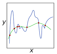
Need for regularization. In some practical situations, based on the measurement results, we can determine all the model’s parameters with reasonably accuracy. However, in many other situations, the inverse problem is ill-defined in the sense that several very different combinations of parameters are consistent with all the measurement results.
This happens, e.g., in dynamical systems, when the observations provide a smoothed picture of the system’s dynamics. For example, if we are tracing the motion of a mechanical system caused by an external force, then a strong but short-time force in one direction followed by a similar strong and short-time force in the opposite direction will (almost) cancel each other, so the same almost-unchanging behavior is consistent both with the absence of forces and with the above wildly-oscillating force. A similar phenomenon occurs when, based on the observed economic behavior, we try to reconstruct the external forces affecting the economic system.
In such situations, the only way to narrow down the set of possible solutions is to take into account some general a priori information. For example, for forces, we may know-e.g., from experts-the upper bound on each individual force, or the upper bound on the overall force. The use of such a priori information is known as regularization; see, e.g., Tikhonov and Arsenin (1977).
金融代写|金融计量经济学Financial Econometrics代考|General and Probabilistic Regularizations
General idea of regularization and its possible probabilistic background. In general, regularization means that we dismiss values $a_{i}$ which are too large or too small. In some cases, this dismissal is based on subjective estimations of what is large and what is small. In other cases, the conclusion about what is large and what is not large is based on past experience of solving similar problem-i.e., on our estimate of the frequencies (= probabilities) with which different values have been observed in the past. In this paper, we consider both types of regularization.
Probabilistic regularization: towards a precise definition. There is no a priori reason to believe that different parameters have different distributions. So, in the first approximation, it makes sense to assume that they have the same probability distribution. Let us denote the probability density function of this common distribution by $\rho(a)$.
In more precise terms, the original information is invariant with respect to all possible permutations of the parameters; thus, it makes sense to conclude that the resulting joint distribution is also invariant with respect to all these permutationswhich implies, in particular, that all the marginal distributions are the same.
Similarly, in general, we do not have a priori reasons to prefer positive or negative values of each the coefficients, i.e., the a priori information is invariant with respect to changing the sign of each of the variables: $a_{i} \rightarrow-a_{i}$. It is therefore reasonable to conclude that the marginal distribution should also be invariant, i.e., that we should have $\rho(-a)=\rho(a)$, and thus, $\rho(a)=\rho(|a|)$.
Also, there is no reason to believe that different parameters are positively or negatively correlated, so it makes sense to assume that their distributions are statistically independent. This is in line with the general Maximum Entropy (=Laplace Indeterminacy Principle) ideas Jaynes and Bretthorst (2003), according to which we should not pretend to be certain – to be more precise, if several different probability distributions are consistent with our knowledge:
- we should not select distributions with small entropy (measure of uncertainty),
- we should select the one for which the entropy is the largest.
If all we know are marginal distributions, then this principle leads to the conclusion that the corresponding variables are independent; see, e.g., Jaynes and Bretthorst $(2003) .$
Due to the independence assumption, the joint distribution of $n$ variables $a_{i}$ take the form $\rho\left(a_{0}, a_{1}, \ldots, a_{n}\right)=\prod_{i=0}^{n} \rho\left(\left|a_{i}\right|\right)$. In applications of probability and statistics, it is usually assumed, crudely speaking, that events with very small probability are not expected to happen. This is the basis for all statistical tests-e.g., if we assume that the distribution is normal with given mean and standard deviation, and the probability that this distribution will lead to the observed data is very small (e.g., if we observe a 5 -sigma deviation from the mean), then we can conclude, with high confidence, that experiments disprove our assumption. In other words, we take some threshold $t_{0}$, and we consider only the tuples $a=\left(a_{0}, a_{1}, \ldots, a_{n}\right)$ for which $\rho\left(a_{0}, a_{1}, \ldots, a_{n}\right)=$ $\prod_{i=0}^{n} \rho\left(\left|a_{i}\right|\right) \geq t_{0}$. By taking logarithms of both sides and changing signs, we get an equivalent inequality
$$
\sum_{i=0}^{n} \psi\left(\left|a_{i}\right|\right) \leq p_{0}
$$
金融代写|金融计量经济学Financial Econometrics代考|Natural Invariances
Scale-invariance: general idea. The numerical values of physical quantities depend on the selection of a measuring unit. For example, if we previously used meters and now start using centimeters, all the physical quantities will remain the same, but the numerical values will change-they will all get multiplied by 100 .
In general, if we replace the original measuring unit with a new measuring unit which is $\lambda$ times smaller, then all the numerical values get multiplied by $\lambda$ :
$$
x \rightarrow x^{\prime}=\lambda \cdot x
$$
Similarly, if we change the original measuring units for the quantity $y$ to a new unit which is $\lambda$ times smaller, then all the coefficients $a_{i}$ in the corresponding dependence $y=a_{0}+\cdots+a_{i} \cdot x_{i}+\cdots$ will also be multiplied by the same factor: $a_{i} \rightarrow \lambda \cdot a_{i}$.
Scale-invariance: case of probabilistic constraints. It is reasonable to require that the corresponding constraints should not depend on the choice of a measuring unit. Of course, if we change $a_{i}$ to $\lambda \cdot a_{i}$, then the value $p_{0}$ may also need to be accordingly changed, but overall, the constraint should remain the same. Thus, we arrive at the following definition.
Definition 4 We say that probability constraints corresponding to the function $\psi(z)$ are scale-invariant if for every $p_{0}$ and for every $\lambda>0$, there exists a value $p_{0}^{\prime}$ such that
$$
\sum_{i=0}^{n} \psi\left(\left|a_{i}\right|\right)=p_{0} \Leftrightarrow \sum_{i=0}^{n} \psi\left(\lambda \cdot\left|a_{i}\right|\right)=p_{0}^{\prime}
$$
Scale-invariance: case of general constraints. In general, the degree of impossibility is described in the same units as the coefficients themselves. Thus, invariance would mean that if replace $a$ and $b$ with $\lambda \cdot a$ and $\lambda \cdot b$, then the combined value $a * b$ will be replaced by a similarly re-scaled value $\lambda \cdot(a * b)$. Thus, we arrive at the following definition.
金融计量经济学代考
金融代写|金融计量经济学Financial Econometrics代考|Formulation of the Problem
需要解决逆问题。一旦我们有了一个系统的模型,我们就可以使用这个模型来预测系统的行为,特别是预测这个系统未来测量和观察的结果。基于模型估计未来测量结果的问题称为前向问题。
在许多实际情况下,我们不知道确切的模型。更准确地说,我们知道物理量之间依赖关系的一般形式,但这种依赖关系的参数需要从观察和实验结果中确定。例如,通常,我们有一个线性模型是= 一个0+∑一世=1n一个一世⋅X一世, 其中参数一个一世需要通过实验确定。根据测量结果确定模型参数的问题称为逆问题。
为了实际找到参数,我们可以使用例如最大似然法。例如,当误差呈正态分布时,最大似然过程会产生通常的最小二乘估计;见,例如,Sheskin (2011). F○̄́ 和X一个̄米p̄l和́, F○̄r 一个̄ G和n和n和́r一个̆l l一世ñ和一个rr 米○几个对应值的元组(X1(ķ),…,Xn(ķ),是(ķ)),1≤ķ≤ķ, 那么我们可以从
$$
\sum_{k=1}^{K}\left(y^{(k)}-\left(a_{0}+\sum_{i=1} ^{n} a_{i} \cdot x_{i}^{(k)}\right)\right)^{2} \rightarrow \min {a {0}, \ldots, a_{n}}
$$
需要正则化。在一些实际情况下,根据测量结果,我们可以相当准确地确定模型的所有参数。然而,在许多其他情况下,逆问题是不明确的,因为参数的几个非常不同的组合与所有测量结果一致。
例如,在动态系统中,当观测提供系统动态的平滑图像时,就会发生这种情况。例如,如果我们正在追踪由外力引起的机械系统的运动,那么在一个方向上的强而短时间的力,随后在相反方向上的类似强而短时间的力将(几乎)抵消每个其他,因此相同的几乎不变的行为与没有力和上述剧烈振荡的力一致。当我们根据观察到的经济行为,试图重构影响经济系统的外力时,也会出现类似的现象。
在这种情况下,缩小可能解决方案的范围的唯一方法是考虑一些一般的先验信息。例如,对于力,我们可能知道(例如,从专家那里)每个单独力的上限,或整体力的上限。这种先验信息的使用称为正则化;例如,参见 Tikhonov 和 Arsenin (1977)。
金融代写|金融计量经济学Financial Econometrics代考|General and Probabilistic Regularizations
正则化的一般概念及其可能的概率背景。一般来说,正则化意味着我们忽略值一个一世太大或太小。在某些情况下,这种解雇是基于对什么是大什么是小的主观估计。在其他情况下,关于什么是大什么不是大的结论是基于过去解决类似问题的经验——即,基于我们对过去观察到不同值的频率(=概率)的估计。在本文中,我们考虑了这两种类型的正则化。
概率正则化:走向精确定义。没有先验理由相信不同的参数有不同的分布。因此,在第一个近似值中,假设它们具有相同的概率分布是有意义的。让我们将这个共同分布的概率密度函数表示为ρ(一个).
更准确地说,原始信息对于参数的所有可能排列是不变的;因此,得出这样的结论是有意义的,即由此产生的联合分布对于所有这些排列也是不变的,这尤其意味着所有边缘分布都是相同的。
类似地,一般来说,我们没有先验理由偏爱每个系数的正值或负值,即先验信息在改变每个变量的符号方面是不变的:一个一世→−一个一世. 因此可以合理地得出结论,边际分布也应该是不变的,即我们应该有ρ(−一个)=ρ(一个), 因此,ρ(一个)=ρ(|一个|).
此外,没有理由相信不同的参数是正相关或负相关,因此假设它们的分布在统计上是独立的是有意义的。这与一般最大熵(=拉普拉斯不确定性原理)思想 Jaynes 和 Bretthorst (2003) 一致,根据该思想,我们不应该假装确定——更准确地说,如果几个不同的概率分布与我们的知识一致:
- 我们不应该选择熵小的分布(不确定性的度量),
- 我们应该选择熵最大的那个。
如果我们所知道的只是边际分布,那么这个原理就会得出相应变量是独立的结论;例如,参见 Jaynes 和 Bretthorst(2003).
由于独立性假设,联合分布n变量一个一世采取形式ρ(一个0,一个1,…,一个n)=∏一世=0nρ(|一个一世|). 在概率和统计的应用中,粗略地说,通常假设概率很小的事件不会发生。这是所有统计检验的基础——例如,如果我们假设分布在给定均值和标准差的情况下是正态分布,并且这种分布导致观察到的数据的概率非常小(例如,如果我们观察到 5 – sigma 偏差),那么我们可以很有信心地得出结论,实验证明了我们的假设。换句话说,我们采取一些阈值吨0, 我们只考虑元组一个=(一个0,一个1,…,一个n)为此ρ(一个0,一个1,…,一个n)= ∏一世=0nρ(|一个一世|)≥吨0. 取两边的对数并改变符号,我们得到一个等价的不等式
∑一世=0nψ(|一个一世|)≤p0
金融代写|金融计量经济学Financial Econometrics代考|Natural Invariances
尺度不变性:一般概念。物理量的数值取决于测量单位的选择。例如,如果我们以前使用米,现在开始使用厘米,所有物理量都将保持不变,但数值会发生变化——它们都会乘以 100。
一般来说,如果我们用一个新的测量单位替换原来的测量单位,即λ倍小,然后所有数值乘以λ :
X→X′=λ⋅X
同样,如果我们改变数量的原始计量单位是到一个新单位λ倍小,然后是所有系数一个一世在相应的依赖中是=一个0+⋯+一个一世⋅X一世+⋯也将乘以相同的因子:一个一世→λ⋅一个一世.
尺度不变性:概率约束的情况。要求相应的约束不应依赖于测量单位的选择是合理的。当然,如果我们改变一个一世至λ⋅一个一世, 那么值p0可能也需要相应地更改,但总的来说,约束应该保持不变。因此,我们得出以下定义。
定义4 我们说对应于函数的概率约束ψ(和)是尺度不变的,如果对于每个p0并且对于每个λ>0, 存在一个值p0′这样
∑一世=0nψ(|一个一世|)=p0⇔∑一世=0nψ(λ⋅|一个一世|)=p0′
尺度不变性:一般约束的情况。通常,不可能的程度与系数本身的单位相同。因此,不变性意味着如果替换一个和b和λ⋅一个和λ⋅b,然后是组合值一个∗b将被类似重新缩放的值替换λ⋅(一个∗b). 因此,我们得出以下定义。

统计代写请认准statistics-lab™. statistics-lab™为您的留学生涯保驾护航。
金融工程代写
金融工程是使用数学技术来解决金融问题。金融工程使用计算机科学、统计学、经济学和应用数学领域的工具和知识来解决当前的金融问题,以及设计新的和创新的金融产品。
非参数统计代写
非参数统计指的是一种统计方法,其中不假设数据来自于由少数参数决定的规定模型;这种模型的例子包括正态分布模型和线性回归模型。
广义线性模型代考
广义线性模型(GLM)归属统计学领域,是一种应用灵活的线性回归模型。该模型允许因变量的偏差分布有除了正态分布之外的其它分布。
术语 广义线性模型(GLM)通常是指给定连续和/或分类预测因素的连续响应变量的常规线性回归模型。它包括多元线性回归,以及方差分析和方差分析(仅含固定效应)。
有限元方法代写
有限元方法(FEM)是一种流行的方法,用于数值解决工程和数学建模中出现的微分方程。典型的问题领域包括结构分析、传热、流体流动、质量运输和电磁势等传统领域。
有限元是一种通用的数值方法,用于解决两个或三个空间变量的偏微分方程(即一些边界值问题)。为了解决一个问题,有限元将一个大系统细分为更小、更简单的部分,称为有限元。这是通过在空间维度上的特定空间离散化来实现的,它是通过构建对象的网格来实现的:用于求解的数值域,它有有限数量的点。边界值问题的有限元方法表述最终导致一个代数方程组。该方法在域上对未知函数进行逼近。[1] 然后将模拟这些有限元的简单方程组合成一个更大的方程系统,以模拟整个问题。然后,有限元通过变化微积分使相关的误差函数最小化来逼近一个解决方案。
tatistics-lab作为专业的留学生服务机构,多年来已为美国、英国、加拿大、澳洲等留学热门地的学生提供专业的学术服务,包括但不限于Essay代写,Assignment代写,Dissertation代写,Report代写,小组作业代写,Proposal代写,Paper代写,Presentation代写,计算机作业代写,论文修改和润色,网课代做,exam代考等等。写作范围涵盖高中,本科,研究生等海外留学全阶段,辐射金融,经济学,会计学,审计学,管理学等全球99%专业科目。写作团队既有专业英语母语作者,也有海外名校硕博留学生,每位写作老师都拥有过硬的语言能力,专业的学科背景和学术写作经验。我们承诺100%原创,100%专业,100%准时,100%满意。
随机分析代写
随机微积分是数学的一个分支,对随机过程进行操作。它允许为随机过程的积分定义一个关于随机过程的一致的积分理论。这个领域是由日本数学家伊藤清在第二次世界大战期间创建并开始的。
时间序列分析代写
随机过程,是依赖于参数的一组随机变量的全体,参数通常是时间。 随机变量是随机现象的数量表现,其时间序列是一组按照时间发生先后顺序进行排列的数据点序列。通常一组时间序列的时间间隔为一恒定值(如1秒,5分钟,12小时,7天,1年),因此时间序列可以作为离散时间数据进行分析处理。研究时间序列数据的意义在于现实中,往往需要研究某个事物其随时间发展变化的规律。这就需要通过研究该事物过去发展的历史记录,以得到其自身发展的规律。
回归分析代写
多元回归分析渐进(Multiple Regression Analysis Asymptotics)属于计量经济学领域,主要是一种数学上的统计分析方法,可以分析复杂情况下各影响因素的数学关系,在自然科学、社会和经济学等多个领域内应用广泛。
MATLAB代写
MATLAB 是一种用于技术计算的高性能语言。它将计算、可视化和编程集成在一个易于使用的环境中,其中问题和解决方案以熟悉的数学符号表示。典型用途包括:数学和计算算法开发建模、仿真和原型制作数据分析、探索和可视化科学和工程图形应用程序开发,包括图形用户界面构建MATLAB 是一个交互式系统,其基本数据元素是一个不需要维度的数组。这使您可以解决许多技术计算问题,尤其是那些具有矩阵和向量公式的问题,而只需用 C 或 Fortran 等标量非交互式语言编写程序所需的时间的一小部分。MATLAB 名称代表矩阵实验室。MATLAB 最初的编写目的是提供对由 LINPACK 和 EISPACK 项目开发的矩阵软件的轻松访问,这两个项目共同代表了矩阵计算软件的最新技术。MATLAB 经过多年的发展,得到了许多用户的投入。在大学环境中,它是数学、工程和科学入门和高级课程的标准教学工具。在工业领域,MATLAB 是高效研究、开发和分析的首选工具。MATLAB 具有一系列称为工具箱的特定于应用程序的解决方案。对于大多数 MATLAB 用户来说非常重要,工具箱允许您学习和应用专业技术。工具箱是 MATLAB 函数(M 文件)的综合集合,可扩展 MATLAB 环境以解决特定类别的问题。可用工具箱的领域包括信号处理、控制系统、神经网络、模糊逻辑、小波、仿真等。