如果你也在 怎样代写工程统计engineering statistics这个学科遇到相关的难题,请随时右上角联系我们的24/7代写客服。
工程统计结合了工程和统计,使用科学方法分析数据。工程统计涉及有关制造过程的数据,如:部件尺寸、公差、材料类型和制造过程控制。
statistics-lab™ 为您的留学生涯保驾护航 在代写工程统计engineering statistics方面已经树立了自己的口碑, 保证靠谱, 高质且原创的统计Statistics代写服务。我们的专家在代写工程统计engineering statistics代写方面经验极为丰富,各种代写工程统计engineering statistics相关的作业也就用不着说。
我们提供的工程统计engineering statistics及其相关学科的代写,服务范围广, 其中包括但不限于:
- Statistical Inference 统计推断
- Statistical Computing 统计计算
- Advanced Probability Theory 高等概率论
- Advanced Mathematical Statistics 高等数理统计学
- (Generalized) Linear Models 广义线性模型
- Statistical Machine Learning 统计机器学习
- Longitudinal Data Analysis 纵向数据分析
- Foundations of Data Science 数据科学基础
统计代写|工程统计代写engineering statistics代考|CONTINUOUS MODELS
Continuous distributions are more important in industrial experiments and research studies. Measurement of quantities (like height, weight, length, temperature, conductivity, resistance, etc.) on the ratio scale is continuous or quantitative data.
Definition 1.1 The stochastic variable that underlies quantitative data is called a continuous random variable, as they can take a continuum of possible values in a finite or infinite interval with an associated probability.
This can be thought of as the limiting form of a point probability function, as the possible values of the underlying continuous random variable become more and more of fine granularity. Thus, the mark in an exam (say between 0 and 100 ) is assumed to be a continuous random variable, even if fractional marks are not permitted. In other words, marks can be modeled by a continuous law even though it is not measured at the finest possible granularity level of fractions. If all students scored between 50 and 100 in an exam, the observed range for that exam is of course $50 \leq x \leq 100$. This range may vary from exam to exam, so that the lower limit could differ from 50 , and the upper limit of 100 is never achieved (nobody got a perfect 100 ). This range is in fact immaterial in several statistical procedures.
All continuous variables need not follow a statistical law. But there are many chance phenomena and physical laws that can be approximated by one of the continuous distributions like the normal law, if not exact. For instance, errors in various measurements are assumed to be normally distributed with zero mean. Similarly, symmetric measurement variations in physical properties like diameter, size of manufactured products, exceedences of dams and reservoirs, and so on, are assumed to follow a continuous uniform law centered around an ideal value $\theta$. This is because they can vary in both directions from an ideal value called its central value.
统计代写|工程统计代写engineering statistics代考|STANDARD DISTRIBUTIONS
Most of the statistical distributions have one or more parameters. These parameters describe the location (central tendency), spread (dispersion), and other shape characteristics of the distribution. There exist several distributions for which the location information is captured by one, and scale information by another parameter. These are called location-and-scale (LaS) distributions (page 7). There are some distributions called standard probability distributions (SPD) for which the parameters are universally fixed. This applies not only to LaS distributions, but to others as well.
Definition 1.2 A standard probability distribution is a specific member of a parametric family in which all the parameters are fixed so that every member of the family can be obtained by arithmetic transformations of variates.
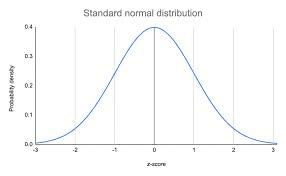
These are also called “parameter-free” distributions (although location parameter is most often 0 , and scale parameter is 1). Examples in univariate case are the standard normal $\mathrm{N}(0,1)$ with PDF $f(z)=(1 / \sqrt{2 \pi}) \exp \left(-z^{2} / 2\right)$, for which location parameter is 0 , and scale parameter is 1 ; unit rectangular $\mathrm{U}(0,1)$, standard exponential distribution (SED) with PDF $f(x)=$ $\exp (-x)$, standard Laplace distribution with PDF $f(x)=\frac{1}{2} \exp (-|x|)$, standard Cauchy distribution with PDF $f(x)=1 /\left(\pi\left(1+x^{2}\right)\right)$, standard lognormal distribution with PDF $f(x)=$ $\exp \left(-(\log (x))^{2} / 2\right) /(\sqrt{2 \pi} x)$, and so on. This concept can easily be extended to the bivariate and multivariate probability distributions too. Simple change of origin and scale transformation can be used on the SPD to obtain all other members of its family as $X=\mu+\sigma Z$. Not all statistical distributions have meaningful SPD forms, however. Examples are $\chi^{2}, F$, and $T$ distributions that depend on one or more degrees of freedom (DoF) parameters, and gamma distribution with two parameters that has PDF $f(x ; a, m)=a^{m} x^{m-1} \exp (-a x) / \Gamma(m)$. This is because setting special values to the respective parameters results in other distributions. ${ }^{2}$ As examples, the $\mathrm{T}$ distribution becomes Cauchy distribution for DoF $n=1$, and $\chi^{2}$ distribution with $n=2$ becomes exponential distribution with parameter $1 / 2$.
The notion of SPD is important from many perspectives: (i) tables of the distributions are easily developed for standard forms; (ii) all parametric families of a distribution can be obtained from the SPD form using appropriate variate transformations; (iii) asymptotic convergence of various distributions are better understood using the SPD (for instance, the Student’s $t$ distribution tends to the standard normal when the DoF parameter becomes large); and (iv) test statistics and confidence intervals used in statistical inference are easier derived using the respective SPD.
统计代写|工程统计代写engineering statistics代考|TAIL AREAS
The area from the lower limit to a particular value of $x$ is called the CDF (left-tail area). It is called “probability content” in physics and some engineering fields, although statisticians seem to use “probability content” to mean the volume under bivariate or multivariate distributions. The PDF is usually denoted by lowercase English letters, and the CDF by uppercase letters. Thus, $f(x ; \mu)$ denotes the PDF (called Lebesque density in some fields), and $F(x ; \mu)=$ $\int_{l l}^{x} f(y) d y=\int_{l l}^{x} d F(y)$, where $l l$ is the lower limit, the CDF ( $\mu$ denotes unknown parameters). It follows that $(\partial / \partial x) F(x)=f(x)$, and $\operatorname{Pr}[a<X \leq b]=F(b)-F(a)=\int_{a}^{b} f(x) d x$. The differential operator $d x, d y$, etc. are written in the beginning in some non-mathematics fields (especially physics, astronomy, etc.) as $F(x ; \mu)=\int_{l l}^{x} d y f(y)$. Although a notational issue, we will use it at the end of an integral, especially in multiple integrals involving $d x d y$, etc. The quantity $f(x) d x$ is called probability differential in physical sciences. Note that $f(x)$ (density function evaluated at a particular value of $x$ within its domain) need not represent a probability, and in fact could sometimes exceed one in magnitude. For instance, Beta-I $(p, q)$ for $p=8, q=3$ evaluated at $x=0.855$ returns $2.528141$. However, $f(x) d x$ always represents the probability $\operatorname{Pr}(x-d x / 2 \leq X \leq x+d x / 2)$, which is in $[0,1]$.
Alternate notations for the PDF are $f(x \mid \mu), f_{x}(\mu)$, and $f(x ; \mu) d x$, and corresponding $\mathrm{CDF}$ are $F(x \mid \mu)$ and $F_{x}(\mu)$. These are written simply as $f(x)$ and $F(x)$ when general statements (without regard to the parameters) are made that hold for all continuous distributions. If $X$ is any continuous random variable with CDF $F(x)$, then $U=F(x) \sim U[0,1]$ (Chapter 2). This fact is used to generate random numbers from continuous distributions when the CDF or SF has closed form. The right-tail area (i.e., SF) is denoted by $S(x)$. As the total area is unity, we get $F(x)+S(x)=1$. Many other functions are defined in terms of $F(x)$ or $S(x)$. The hazard function used in reliability is defined as
$$
h(x)=f(x) /(1-F(x))=f(x) / S(x)
$$
工程统计代考
统计代写|工程统计代写engineering statistics代考|CONTINUOUS MODELS
连续分布在工业实验和研究中更为重要。比例尺上的量(如高度、重量、长度、温度、电导率、电阻等)的测量是连续的或定量的数据。
定义 1.1 构成定量数据基础的随机变量称为连续随机变量,因为它们可以在具有相关概率的有限或无限区间内获取连续的可能值。
这可以被认为是点概率函数的极限形式,因为底层连续随机变量的可能值变得越来越细粒度。因此,考试中的分数(例如 0 到 100 之间)被假定为连续随机变量,即使分数分数是不允许的。换句话说,标记可以通过连续定律建模,即使它不是在可能的最细粒度级别的分数上测量的。如果所有学生在考试中得分在 50 到 100 之间,那么该考试的观测范围当然是50≤X≤100. 这个范围可能因考试而异,因此下限可能与 50 不同,并且永远不会达到 100 的上限(没有人得到完美的 100 )。这个范围实际上在一些统计程序中并不重要。
所有连续变量都不需要遵循统计规律。但是有许多偶然现象和物理定律可以通过像正态定律这样的连续分布之一来近似,如果不精确的话。例如,假设各种测量中的误差呈正态分布,均值为零。类似地,物理特性的对称测量变化,如直径、制成品的尺寸、水坝和水库的超出范围等,被假定遵循以理想值为中心的连续均匀定律θ. 这是因为它们可以从称为中心值的理想值在两个方向上变化。
统计代写|工程统计代写engineering statistics代考|STANDARD DISTRIBUTIONS
大多数统计分布都有一个或多个参数。这些参数描述了分布的位置(集中趋势)、散布(分散)和其他形状特征。存在几种分布,其中位置信息由一个捕获,而尺度信息由另一个参数捕获。这些称为位置和规模 (LaS) 分布(第 7 页)。有一些分布称为标准概率分布 (SPD),其参数是普遍固定的。这不仅适用于 LaS 发行版,也适用于其他发行版。
定义 1.2 标准概率分布是参数族的特定成员,其中所有参数都是固定的,因此该族的每个成员都可以通过变量的算术变换获得。
这些也称为“无参数”分布(尽管位置参数通常为 0,尺度参数为 1)。单变量情况下的示例是标准正态ñ(0,1)带PDFF(和)=(1/2圆周率)经验(−和2/2), 其中位置参数为 0 , 尺度参数为 1 ; 单位 长方形在(0,1), 标准指数分布 (SED) 与 PDFF(X)= 经验(−X), 标准拉普拉斯分布与 PDFF(X)=12经验(−|X|), 标准柯西分布与 PDFF(X)=1/(圆周率(1+X2)), 标准对数正态分布与 PDFF(X)= 经验(−(日志(X))2/2)/(2圆周率X), 等等。这个概念也可以很容易地扩展到双变量和多变量概率分布。可以在 SPD 上使用简单的原点变化和比例变换来获得其家族的所有其他成员:X=μ+σ从. 然而,并非所有统计分布都具有有意义的 SPD 形式。例子是χ2,F, 和吨取决于一个或多个自由度 (DoF) 参数的分布,以及具有 PDF 的两个参数的伽马分布F(X;一个,米)=一个米X米−1经验(−一个X)/Γ(米). 这是因为为各个参数设置特殊值会导致其他分布。2例如,吨分布变为自由度的柯西分布n=1, 和χ2分布与n=2变成带参数的指数分布1/2.
从许多角度来看,SPD 的概念都很重要:(i) 分布表很容易为标准形式开发;(ii) 可以使用适当的变量变换从 SPD 形式获得分布的所有参数族;(iii) 使用 SPD 可以更好地理解各种分布的渐近收敛(例如,Student’s吨自由度参数变大时分布趋于标准正态);(iv) 统计推断中使用的测试统计量和置信区间更容易使用相应的 SPD 导出。
统计代写|工程统计代写engineering statistics代考|TAIL AREAS
从下限到特定值的区域X称为CDF(左尾区)。它在物理学和一些工程领域被称为“概率内容”,尽管统计学家似乎使用“概率内容”来表示二元或多变量分布下的体积。PDF 通常用小写英文字母表示,CDF 用大写字母表示。因此,F(X;μ)表示 PDF(在某些领域称为 Lebesque 密度),并且F(X;μ)= ∫llXF(是)d是=∫llXdF(是), 在哪里ll是下限,CDF (μ表示未知参数)。它遵循(∂/∂X)F(X)=F(X), 和公关[一个<X≤b]=F(b)−F(一个)=∫一个bF(X)dX. 微分算子dX,d是等在一些非数学领域(尤其是物理学、天文学等)一开始就写成F(X;μ)=∫llXd是F(是). 虽然是一个符号问题,但我们将在积分的末尾使用它,尤其是在涉及的多重积分中dXd是等数量F(X)dX在物理科学中称为概率微分。注意F(X)(密度函数在特定值评估X在其域内)不需要表示概率,实际上有时可能会超过 1。例如,Beta-I(p,q)为了p=8,q=3评价为X=0.855返回2.528141. 然而,F(X)dX总是代表概率公关(X−dX/2≤X≤X+dX/2),这是在[0,1].
PDF 的替代符号是F(X∣μ),FX(μ), 和F(X;μ)dX, 和对应的CDF是F(X∣μ)和FX(μ). 这些简单地写成F(X)和F(X)当做出适用于所有连续分布的一般陈述(不考虑参数)时。如果X是任何具有 CDF 的连续随机变量F(X), 然后在=F(X)∼在[0,1](第2章)。当 CDF 或 SF 具有闭合形式时,此事实用于从连续分布中生成随机数。右尾区域(即SF)表示为小号(X). 由于总面积是一单位,我们得到F(X)+小号(X)=1. 许多其他功能是根据以下定义的F(X)或者小号(X). 可靠性中使用的风险函数定义为
H(X)=F(X)/(1−F(X))=F(X)/小号(X)

统计代写请认准statistics-lab™. statistics-lab™为您的留学生涯保驾护航。
金融工程代写
金融工程是使用数学技术来解决金融问题。金融工程使用计算机科学、统计学、经济学和应用数学领域的工具和知识来解决当前的金融问题,以及设计新的和创新的金融产品。
非参数统计代写
非参数统计指的是一种统计方法,其中不假设数据来自于由少数参数决定的规定模型;这种模型的例子包括正态分布模型和线性回归模型。
广义线性模型代考
广义线性模型(GLM)归属统计学领域,是一种应用灵活的线性回归模型。该模型允许因变量的偏差分布有除了正态分布之外的其它分布。
术语 广义线性模型(GLM)通常是指给定连续和/或分类预测因素的连续响应变量的常规线性回归模型。它包括多元线性回归,以及方差分析和方差分析(仅含固定效应)。
有限元方法代写
有限元方法(FEM)是一种流行的方法,用于数值解决工程和数学建模中出现的微分方程。典型的问题领域包括结构分析、传热、流体流动、质量运输和电磁势等传统领域。
有限元是一种通用的数值方法,用于解决两个或三个空间变量的偏微分方程(即一些边界值问题)。为了解决一个问题,有限元将一个大系统细分为更小、更简单的部分,称为有限元。这是通过在空间维度上的特定空间离散化来实现的,它是通过构建对象的网格来实现的:用于求解的数值域,它有有限数量的点。边界值问题的有限元方法表述最终导致一个代数方程组。该方法在域上对未知函数进行逼近。[1] 然后将模拟这些有限元的简单方程组合成一个更大的方程系统,以模拟整个问题。然后,有限元通过变化微积分使相关的误差函数最小化来逼近一个解决方案。
tatistics-lab作为专业的留学生服务机构,多年来已为美国、英国、加拿大、澳洲等留学热门地的学生提供专业的学术服务,包括但不限于Essay代写,Assignment代写,Dissertation代写,Report代写,小组作业代写,Proposal代写,Paper代写,Presentation代写,计算机作业代写,论文修改和润色,网课代做,exam代考等等。写作范围涵盖高中,本科,研究生等海外留学全阶段,辐射金融,经济学,会计学,审计学,管理学等全球99%专业科目。写作团队既有专业英语母语作者,也有海外名校硕博留学生,每位写作老师都拥有过硬的语言能力,专业的学科背景和学术写作经验。我们承诺100%原创,100%专业,100%准时,100%满意。
随机分析代写
随机微积分是数学的一个分支,对随机过程进行操作。它允许为随机过程的积分定义一个关于随机过程的一致的积分理论。这个领域是由日本数学家伊藤清在第二次世界大战期间创建并开始的。
时间序列分析代写
随机过程,是依赖于参数的一组随机变量的全体,参数通常是时间。 随机变量是随机现象的数量表现,其时间序列是一组按照时间发生先后顺序进行排列的数据点序列。通常一组时间序列的时间间隔为一恒定值(如1秒,5分钟,12小时,7天,1年),因此时间序列可以作为离散时间数据进行分析处理。研究时间序列数据的意义在于现实中,往往需要研究某个事物其随时间发展变化的规律。这就需要通过研究该事物过去发展的历史记录,以得到其自身发展的规律。
回归分析代写
多元回归分析渐进(Multiple Regression Analysis Asymptotics)属于计量经济学领域,主要是一种数学上的统计分析方法,可以分析复杂情况下各影响因素的数学关系,在自然科学、社会和经济学等多个领域内应用广泛。
MATLAB代写
MATLAB 是一种用于技术计算的高性能语言。它将计算、可视化和编程集成在一个易于使用的环境中,其中问题和解决方案以熟悉的数学符号表示。典型用途包括:数学和计算算法开发建模、仿真和原型制作数据分析、探索和可视化科学和工程图形应用程序开发,包括图形用户界面构建MATLAB 是一个交互式系统,其基本数据元素是一个不需要维度的数组。这使您可以解决许多技术计算问题,尤其是那些具有矩阵和向量公式的问题,而只需用 C 或 Fortran 等标量非交互式语言编写程序所需的时间的一小部分。MATLAB 名称代表矩阵实验室。MATLAB 最初的编写目的是提供对由 LINPACK 和 EISPACK 项目开发的矩阵软件的轻松访问,这两个项目共同代表了矩阵计算软件的最新技术。MATLAB 经过多年的发展,得到了许多用户的投入。在大学环境中,它是数学、工程和科学入门和高级课程的标准教学工具。在工业领域,MATLAB 是高效研究、开发和分析的首选工具。MATLAB 具有一系列称为工具箱的特定于应用程序的解决方案。对于大多数 MATLAB 用户来说非常重要,工具箱允许您学习和应用专业技术。工具箱是 MATLAB 函数(M 文件)的综合集合,可扩展 MATLAB 环境以解决特定类别的问题。可用工具箱的领域包括信号处理、控制系统、神经网络、模糊逻辑、小波、仿真等。