如果你也在 怎样代写电磁学electromagnetism这个学科遇到相关的难题，请随时右上角联系我们的24/7代写客服。

电磁学是电荷、磁矩和电磁场之间的物理互动。电磁场可以是静态的，缓慢变化的，或形成波。电磁波一般被称为光，遵守光学定律。

statistics-lab™ 为您的留学生涯保驾护航 在代写电磁学electromagnetism方面已经树立了自己的口碑, 保证靠谱, 高质且原创的统计Statistics代写服务。我们的专家在代写电磁学electromagnetism代写方面经验极为丰富，各种代写电磁学electromagnetism相关的作业也就用不着说。

我们提供的电磁学electromagnetism及其相关学科的代写，服务范围广, 其中包括但不限于:

• Statistical Inference 统计推断
• Statistical Computing 统计计算
• Advanced Probability Theory 高等概率论
• Advanced Mathematical Statistics 高等数理统计学
• (Generalized) Linear Models 广义线性模型
• Statistical Machine Learning 统计机器学习
• Longitudinal Data Analysis 纵向数据分析
• Foundations of Data Science 数据科学基础

物理代写|电磁学代写electromagnetism代考|Motion in Uniform Electric Field

Suppose a charge particle of mass $m$ and charge $q$ is moving in a uniform electric field $\mathbf{E}$. Electric field $\mathbf{E}$ exerts on a particle placed in it the force
$$
\mathbf{F}=q \mathbf{E}
$$

If that force is equal to the resultant force exerted on the particle, it causes the particle to accelerate, based on Newton’s second law:
$$
m \mathbf{a}=q \mathbf{E}
$$
The acceleration gained by the charge is given as
$$
\mathbf{a}=\frac{q}{m} \mathbf{E}
$$
Therefore, if $\mathbf{E}$ is uniform (that is, constant in magnitude and direction), then a is constant. Furthermore, if the particle has a positive charge, then its acceleration is in the direction of the electric field. On the other hand, if the particle has a negative charge, then its acceleration is in the direction opposite the electric field.

物理代写|电磁学代写electromagnetism代考|Uniform Electric Field

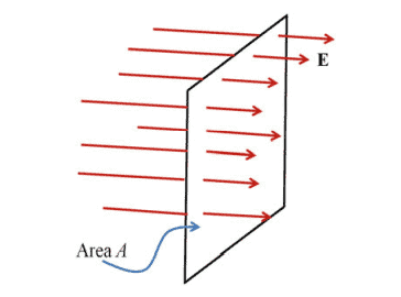
The electric flux concept describes quantitatively the electric lines. The number of field lines per unit area (also called line density) going through a rectangular surface of area $A$, which is perpendicular to the field, is proportional to the magnitude of electric field, E, as shown in Fig. 2.1. Furthermore, the total number of lines penetrating the surface is proportional to the product $|\mathbf{E}|$ A. By definition, the product of the magnitude of electric field $|\mathbf{E}|$ and surface area $A$ perpendicular to the field is called the electric flux:
$$
\Phi_E=|\mathbf{E}| A
$$
Using Eq. (2.1), from the SI units of $E$ and $A$, we derive the SI units of the electric flux:
$$
[E]=\left[\frac{\mathrm{N}}{\mathrm{C}}\right],[A]=\left[\mathrm{m}^2\right]
$$

Thus, we obtain SI units of $\Phi_E$ :
$$
\left[\Phi_E\right]=\left[\frac{\mathrm{N} \cdot \mathrm{m}^2}{\mathrm{C}}\right]
$$
Note that the electric flux is proportional to the number of electric field lines penetrating some surface.

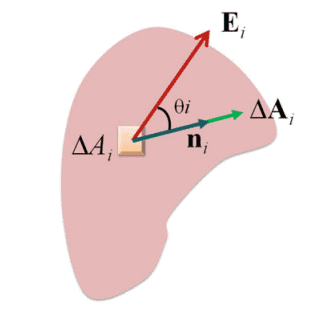
Moreover, consider the electric flux on any surface with an arbitrary orientation with respect to electric field $\mathbf{E}$, as shown in Fig. 2.2. Electric flux going through the surface (with area $A$ ) not perpendicular to $\mathbf{E}$ is smaller than the product $|\mathbf{E}| A$. That is, the number of lines that cross this area $A$ is equal to the number of lines that cross the area $A^{\prime}=A \cos \theta$, which is a projection of $A$ aligned perpendicular to the field. Mathematically, the electric flux is given by (Fig. 2.2)
$$
\Phi_E=|\mathbf{E}| A^{\prime}=|\mathbf{E}| A \cos \theta
$$
From the definition, Eq. (2.4), we can say that the maximum electric flux is achieved when $\theta=0^{\circ}$; that is, the surface is perpendicular to $\mathbf{E}$ : $\Phi_F^{\max }=|\mathbf{E}| A$ (see also Eq. (2.1)). Or, equivalently, when normal vector $\mathbf{n}$ to the surface is parallel to E. On the other hand, the minimum electric flux is achieved when $\theta=90^{\circ}$, that is, the surface is parallel to $\mathbf{E}: \Phi_E^{\min }=0$. In this case, normal vector $\mathbf{n}$ to the surface is perpendicular to $\mathbf{E}$. In general, denoting the vector $\mathbf{A}=A \mathbf{n}$, we can write
$$
\Phi_E=\mathbf{E} \cdot \mathbf{A}
$$

电磁学代考

物理代写|电磁学代写electromagnetism代考|Motion in Uniform Electric Field

假设一个带电粒子的质量 $m$ 并充电 $q$ 在均匀电场中运动 $\mathbf{E}$. 电场E对放置在其中的粒子施加力
$$
\mathbf{F}=q \mathbf{E}
$$
如果该力等于施加在粒子上的合力，它会导致粒子加速，根据牛顿第二定律：
$$
m \mathbf{a}=q \mathbf{E}
$$
电荷获得的加速度为
$$
\mathbf{a}=\frac{q}{m} \mathbf{E}
$$
因此，如果 $\mathbf{E}$ 是均匀的（即大小和方向恒定），则 a 是恒定的。此外，如果粒子带正电荷，则其加速度沿电场 方向。另一方面，如果粒子带负电荷，则其加速度方向与电场相反。

物理代写|电磁学代写electromagnetism代考|Uniform Electric Field

电通量概念定量地描述了电线。穿过矩形表面的每单位面积的场线数 (也称为线密度） $A$ 垂直于场，与电场 $\mathrm{E}$ 的大小成正比，如图 2.1 所示。此外，穿透表面的总线数与产品成正比 $|\mathbf{E}| \mathrm{A}$. 根据定义，电场大小的乘积 $|\mathbf{E}|$ 和 表面积 $A$ 垂直于场的称为电通量:
$$
\Phi_E=|\mathbf{E}| A
$$
使用方程式。(2.1)，从 SI 单位 $E$ 和 $A$ ，我们推导出电通量的 SI 单位:
$$
[E]=\left[\frac{\mathrm{N}}{\mathrm{C}}\right],[A]=\left[\mathrm{m}^2\right]
$$
因此，我们获得了 SI 单位 $\Phi_E$ :
$$
\left[\Phi_E\right]=\left[\frac{\mathrm{N} \cdot \mathrm{m}^2}{\mathrm{C}}\right]
$$
请注意，电通量与穿透某些表面的电场线的数量成正比。
此外，考虑相对于电场具有任意方向的任意表面上的电通量 $\mathbf{E}$ ，如图 $2.2$ 所示。穿过表面的电通量 (面积 $A$ ) 不 垂直于 $\mathbf{E}$ 小于产品 $|\mathbf{E}| A$. 即穿过这个区域的线数 $A$ 等于穿过该区域的线数 $A^{\prime}=A \cos \theta$ ，这是一个投影 $A$ 垂直 于场对旻。在数学上，电通量由下式给出 (图 2.2)
$$
\Phi_E=|\mathbf{E}| A^{\prime}=|\mathbf{E}| A \cos \theta
$$
根据定义，Eq。(2.4)，我们可以说当达到最大电通量时 $\theta=0^{\circ}$; 也就是说，表面垂直于 $\mathbf{E}: \Phi_F^{\max }=|\mathbf{E}| A ＼mathrm{~ 也 ~}$ 见方程式 (2.1）)。或者，等效地，当法向量n到表面平行于 E. 另一方面，当达到最小电通量时 $\theta=90^{\circ} ， 也$ 就是说，表面平行于 $\mathbf{E}: \Phi_E^{\min }=0$. 在这种情况下，法向量 $\mathbf{n}$ 到表面垂直于 $\mathbf{E}$. 一般来说，表示向量 $\mathbf{A}=A \mathbf{n}$, 我们可以写
$$
\Phi_E=\mathbf{E} \cdot \mathbf{A}
$$

统计代写请认准statistics-lab™. statistics-lab™为您的留学生涯保驾护航。

金融工程代写

金融工程是使用数学技术来解决金融问题。金融工程使用计算机科学、统计学、经济学和应用数学领域的工具和知识来解决当前的金融问题，以及设计新的和创新的金融产品。

非参数统计代写

非参数统计指的是一种统计方法，其中不假设数据来自于由少数参数决定的规定模型；这种模型的例子包括正态分布模型和线性回归模型。

广义线性模型代考

广义线性模型（GLM）归属统计学领域，是一种应用灵活的线性回归模型。该模型允许因变量的偏差分布有除了正态分布之外的其它分布。

术语 广义线性模型（GLM）通常是指给定连续和/或分类预测因素的连续响应变量的常规线性回归模型。它包括多元线性回归，以及方差分析和方差分析（仅含固定效应）。

有限元方法代写

有限元方法（FEM）是一种流行的方法，用于数值解决工程和数学建模中出现的微分方程。典型的问题领域包括结构分析、传热、流体流动、质量运输和电磁势等传统领域。

有限元是一种通用的数值方法，用于解决两个或三个空间变量的偏微分方程（即一些边界值问题）。为了解决一个问题，有限元将一个大系统细分为更小、更简单的部分，称为有限元。这是通过在空间维度上的特定空间离散化来实现的，它是通过构建对象的网格来实现的：用于求解的数值域，它有有限数量的点。边界值问题的有限元方法表述最终导致一个代数方程组。该方法在域上对未知函数进行逼近。[1] 然后将模拟这些有限元的简单方程组合成一个更大的方程系统，以模拟整个问题。然后，有限元通过变化微积分使相关的误差函数最小化来逼近一个解决方案。

tatistics-lab作为专业的留学生服务机构，多年来已为美国、英国、加拿大、澳洲等留学热门地的学生提供专业的学术服务，包括但不限于Essay代写，Assignment代写，Dissertation代写，Report代写，小组作业代写，Proposal代写，Paper代写，Presentation代写，计算机作业代写，论文修改和润色，网课代做，exam代考等等。写作范围涵盖高中，本科，研究生等海外留学全阶段，辐射金融，经济学，会计学，审计学，管理学等全球99%专业科目。写作团队既有专业英语母语作者，也有海外名校硕博留学生，每位写作老师都拥有过硬的语言能力，专业的学科背景和学术写作经验。我们承诺100%原创，100%专业，100%准时，100%满意。

随机分析代写

随机微积分是数学的一个分支，对随机过程进行操作。它允许为随机过程的积分定义一个关于随机过程的一致的积分理论。这个领域是由日本数学家伊藤清在第二次世界大战期间创建并开始的。

时间序列分析代写

随机过程，是依赖于参数的一组随机变量的全体，参数通常是时间。 随机变量是随机现象的数量表现，其时间序列是一组按照时间发生先后顺序进行排列的数据点序列。通常一组时间序列的时间间隔为一恒定值（如1秒，5分钟，12小时，7天，1年），因此时间序列可以作为离散时间数据进行分析处理。研究时间序列数据的意义在于现实中，往往需要研究某个事物其随时间发展变化的规律。这就需要通过研究该事物过去发展的历史记录，以得到其自身发展的规律。

回归分析代写

多元回归分析渐进（Multiple Regression Analysis Asymptotics）属于计量经济学领域，主要是一种数学上的统计分析方法，可以分析复杂情况下各影响因素的数学关系，在自然科学、社会和经济学等多个领域内应用广泛。

MATLAB代写

MATLAB 是一种用于技术计算的高性能语言。它将计算、可视化和编程集成在一个易于使用的环境中，其中问题和解决方案以熟悉的数学符号表示。典型用途包括：数学和计算算法开发建模、仿真和原型制作数据分析、探索和可视化科学和工程图形应用程序开发，包括图形用户界面构建MATLAB 是一个交互式系统，其基本数据元素是一个不需要维度的数组。这使您可以解决许多技术计算问题，尤其是那些具有矩阵和向量公式的问题，而只需用 C 或 Fortran 等标量非交互式语言编写程序所需的时间的一小部分。MATLAB 名称代表矩阵实验室。MATLAB 最初的编写目的是提供对由 LINPACK 和 EISPACK 项目开发的矩阵软件的轻松访问，这两个项目共同代表了矩阵计算软件的最新技术。MATLAB 经过多年的发展，得到了许多用户的投入。在大学环境中，它是数学、工程和科学入门和高级课程的标准教学工具。在工业领域，MATLAB 是高效研究、开发和分析的首选工具。MATLAB 具有一系列称为工具箱的特定于应用程序的解决方案。对于大多数 MATLAB 用户来说非常重要，工具箱允许您学习和应用专业技术。工具箱是 MATLAB 函数（M 文件）的综合集合，可扩展 MATLAB 环境以解决特定类别的问题。可用工具箱的领域包括信号处理、控制系统、神经网络、模糊逻辑、小波、仿真等。

R语言代写	问卷设计与分析代写
PYTHON代写	回归分析与线性模型代写
MATLAB代写	方差分析与试验设计代写
STATA代写	机器学习/统计学习代写
SPSS代写	计量经济学代写
EVIEWS代写	时间序列分析代写
EXCEL代写	深度学习代写
SQL代写	各种数据建模与可视化代写

如果你也在 怎样代写电磁学electromagnetism这个学科遇到相关的难题，请随时右上角联系我们的24/7代写客服。

电磁学是电荷、磁矩和电磁场之间的物理互动。电磁场可以是静态的，缓慢变化的，或形成波。电磁波一般被称为光，遵守光学定律。

statistics-lab™ 为您的留学生涯保驾护航 在代写电磁学electromagnetism方面已经树立了自己的口碑, 保证靠谱, 高质且原创的统计Statistics代写服务。我们的专家在代写电磁学electromagnetism代写方面经验极为丰富，各种代写电磁学electromagnetism相关的作业也就用不着说。

我们提供的电磁学electromagnetism及其相关学科的代写，服务范围广, 其中包括但不限于:

• Statistical Inference 统计推断
• Statistical Computing 统计计算
• Advanced Probability Theory 高等概率论
• Advanced Mathematical Statistics 高等数理统计学
• (Generalized) Linear Models 广义线性模型
• Statistical Machine Learning 统计机器学习
• Longitudinal Data Analysis 纵向数据分析
• Foundations of Data Science 数据科学基础

物理代写|电磁学代写electromagnetism代考|Force Fields

The field forces act through space, producing an effect even when no physical contact between the objects occurs. As an example, we can mention the gravitational field. Michael Faraday developed a similar approach to electric forces. That is, an electric field exists in the region of space around any charged body, and when another charged body is inside this region of the electric field, an electric force acts on it.

Definition 1.2 The electric field $\mathbf{E}$ at a point in space is defined as the electric force $\mathbf{F}_e$ acting on a positive test charge $q_0$ placed at that point divided by the magnitude of the test charge:
$$
\mathbf{E}=\frac{\mathbf{F}_e}{q_0}
$$

The vector $\mathbf{E}$ has the SI units of newtons per coulomb (N/C). Figure $1.3$ illustrates the electric field $\mathbf{E}$ created by a positively charged sphere with total charge $Q$ at the positive test charge $q_0$. Here, we have assumed that the test charge $q_0$ is small enough that it does not disturb the charge distribution of the sphere responsible for the electric field.

Note that $\mathbf{E}$ is the field produced by some charge external to the test charge, and it is not the field produced by the test charge itself. Also, note that the existence of an electric field is a property of its source. For example, every electron comes with its electric field. An electric field exists at a point if a test charge at rest at that point experiences an electric force. The electric field direction is the direction of the force on a positive test charge placed in the field. Once we know the magnitude and direction of the electric field at some point, the electric force exerted on any charged particle (either positive or negative) placed at that point can be calculated. The electric field exists at some point space, including the free space, independent of the existence of another test charge at that point.

To determine the direction of electric field, consider a point charge $q$ located some distance $r$ from a test positive charge $q_0$ located at a point $P$, as shown in Fig. 1.4. field Coulomb’s law defines the force exerted by $q$ on $q_0$ as
$$
\mathbf{F}_e=k_e \frac{q q_0}{r^2} \hat{\mathbf{r}}
$$

物理代写|电磁学代写electromagnetism代考|Superposition Principle

According to superposition principle, at any point $P$, the total electric field due to a set of discrete point charges, $q_1, q_2, \ldots, q_N$, positive and negative charges, is equal to the sum of the individual charge electric field vectors (see Fig. 1.5). Mathematically, we can write
$$
\mathbf{E}(\mathbf{r})=\sum_{i=1}^N \mathbf{E}i=\sum{i=1}^N k_e \frac{q_i}{\left|\mathbf{r}-\mathbf{r}_i\right|^2} \hat{\mathbf{r}}_i
$$
In Eq. (1.12), $\left|\mathbf{r}-\mathbf{r}_i\right|$ is the distance from $q_i$ to the point $P$ (the location of a test charge), where $\mathbf{r}$ is the position vector of the point $P$ with respect to some reference frame, as indicated in Fig. 1.5, and $\mathbf{r}_i$ is the position vector of the charge $i$ in that reference frame. Furthermore, $\hat{\mathbf{r}}_i$ is a unit vector directed from $q_i$ toward $P$.

Note that in Eq. (1.12) the dependence of $\mathbf{E}$ on only position vector of point $P, \mathbf{r}$, assumes a static configuration of the charges in space. That is, for some other configuration distribution of charges in space, $\mathbf{E}$ at the same point $P$ may be different. Note that often for convenience, Eq. (1.12) is also written as $$
\mathbf{E}(\mathbf{r})=\sum_{i=1}^N k_e \frac{q_i\left(\mathbf{r}-\mathbf{r}_i\right)}{\left|\mathbf{r}-\mathbf{r}_i\right|^3}
$$
where
$$
\hat{\mathbf{r}}_i=\frac{\mathbf{r}-\mathbf{r}_i}{\left|\mathbf{r}-\mathbf{r}_i\right|}
$$
If the distances between charges in a set of charges are much smaller, compare with the distance of the set from a point where the electric field is to be calculated, then charge distribution is continuous.

电磁学代考

物理代写|电磁学代写electromagnetism代考|Force Fields

场力通过空间发挥作用，即使物体之间没有发生物理接触也会产生影响。作为一个例子，我们可以提到引力场。迈克尔-法拉第开发了一种类似于电场的方法。也就是说，在任何带电体周围的空间中都存在一个电场，当另一个带电体在这个电场区域内时，就有一个电动力作用在它身上。

定义1.2 空间中某一点的电场$mathbf{E}$被定义为作用于放置在该点的正的测试电荷$q_0$的电力量$mathbf{F}_e$除以测试电荷的大小。
$$
\mathbf{E}=\frac{\mathbf{F}_e}{q_0}
$$

矢量$\mathbf{E}$的SI单位为牛顿/库仑（N/C）。图1.3$说明了一个总电荷量为$Q$的带正电的球体在正测试电荷量$q_0$处产生的电场$mathbf{E}$。这里，我们假设测试电荷$q_0$足够小，以至于它不会干扰负责电场的球体的电荷分布。

请注意，$mathbf{E}$是由测试电荷外部的某个电荷产生的场，它不是由测试电荷本身产生的场。另外，请注意，电场的存在是其来源的一个属性。例如，每个电子都有其电场。如果一个静止的测试电荷在某一点经历了一个电动力，那么这个电场就存在于该点。电场方向是指放在电场中的正向测试电荷的受力方向。一旦我们知道了某一点的电场的大小和方向，就可以计算出放在该点的任何带电粒子（无论是正还是负）所受到的电动力。电场存在于某个点的空间，包括自由空间，与该点的另一个测试电荷的存在无关。

为了确定电场的方向，考虑一个点电荷$q$与位于$P$点的测试正电荷$q_0$相距一定距离$r$，如图1.4所示。场库仑定律定义$q$对$q_0$施加的力为
$$
`mathbf{F}_e=k_e `frac{q q_0}{r^2 } \hat{mathbf{r}}}。
$$

物理代写|电磁学代写electromagnetism代考|Superposition Principle

根据叠加原理，在任何一点$P$，一组离散的点电荷$q_1, q_2, \ldots, q_N$（正电荷和负电荷）引起的总电场等于各个电荷电场矢量的总和（见图1.5）。在数学上，我们可以写成
$$
\mathbf{E}(\mathbf{r})=\sum_{i=1}^N \mathbf{E}i=\sum{i=1}^N k_e \frac{q_i}{\left|\mathbf{r}-\mathbf{r}_i\right|^2} \hat{mathbf{r}}_i
$$
在公式（1.12）中，$left|\mathbf{r}-\mathbf{r}_i/right|$是$q_i$到点$P$（测试电荷的位置）的距离，其中$mathbf{r}$是点$P$相对于某个参考框架的位置向量，如图1.5所示，$mathbf{r}_i$是电荷$i$在该参考框架的位置向量。此外，$hat{mathbf{r}}_i$是一个从$q_i$指向$P$的单位矢量。

注意在公式(1.12)中，$mathbf{E}$对$P点的位置向量的依赖，假设空间中电荷的静态配置。也就是说，对于空间中电荷的其他配置分布，同一点$P$的$mathbf{E}$可能是不同的。请注意，为方便起见，公式（1.12）通常也写成$$
\mathbf{E}(\mathbf{r})=\sum_{i=1}^N k_e \frac{q_i\left(\mathbf{r}-\mathbf{r}_i\right)}{\left|\mathbf{r}-\mathbf{r}_i\right|^3}
$$
其中
$$
\hat{\mathbf{r}}_i=\frac{\mathbf{r}-\mathbf{r}_i}{\left|\mathbf{r}-\mathbf{r}_i\right|}
$$
如果一组电荷之间的距离要小得多，与该组电荷离要计算电场的点的距离相比，那么电荷分布是连续的。

统计代写请认准statistics-lab™. statistics-lab™为您的留学生涯保驾护航。

金融工程代写

金融工程是使用数学技术来解决金融问题。金融工程使用计算机科学、统计学、经济学和应用数学领域的工具和知识来解决当前的金融问题，以及设计新的和创新的金融产品。

非参数统计代写

非参数统计指的是一种统计方法，其中不假设数据来自于由少数参数决定的规定模型；这种模型的例子包括正态分布模型和线性回归模型。

广义线性模型代考

广义线性模型（GLM）归属统计学领域，是一种应用灵活的线性回归模型。该模型允许因变量的偏差分布有除了正态分布之外的其它分布。

术语 广义线性模型（GLM）通常是指给定连续和/或分类预测因素的连续响应变量的常规线性回归模型。它包括多元线性回归，以及方差分析和方差分析（仅含固定效应）。

有限元方法代写

有限元方法（FEM）是一种流行的方法，用于数值解决工程和数学建模中出现的微分方程。典型的问题领域包括结构分析、传热、流体流动、质量运输和电磁势等传统领域。

有限元是一种通用的数值方法，用于解决两个或三个空间变量的偏微分方程（即一些边界值问题）。为了解决一个问题，有限元将一个大系统细分为更小、更简单的部分，称为有限元。这是通过在空间维度上的特定空间离散化来实现的，它是通过构建对象的网格来实现的：用于求解的数值域，它有有限数量的点。边界值问题的有限元方法表述最终导致一个代数方程组。该方法在域上对未知函数进行逼近。[1] 然后将模拟这些有限元的简单方程组合成一个更大的方程系统，以模拟整个问题。然后，有限元通过变化微积分使相关的误差函数最小化来逼近一个解决方案。

tatistics-lab作为专业的留学生服务机构，多年来已为美国、英国、加拿大、澳洲等留学热门地的学生提供专业的学术服务，包括但不限于Essay代写，Assignment代写，Dissertation代写，Report代写，小组作业代写，Proposal代写，Paper代写，Presentation代写，计算机作业代写，论文修改和润色，网课代做，exam代考等等。写作范围涵盖高中，本科，研究生等海外留学全阶段，辐射金融，经济学，会计学，审计学，管理学等全球99%专业科目。写作团队既有专业英语母语作者，也有海外名校硕博留学生，每位写作老师都拥有过硬的语言能力，专业的学科背景和学术写作经验。我们承诺100%原创，100%专业，100%准时，100%满意。

随机分析代写

随机微积分是数学的一个分支，对随机过程进行操作。它允许为随机过程的积分定义一个关于随机过程的一致的积分理论。这个领域是由日本数学家伊藤清在第二次世界大战期间创建并开始的。

时间序列分析代写

随机过程，是依赖于参数的一组随机变量的全体，参数通常是时间。 随机变量是随机现象的数量表现，其时间序列是一组按照时间发生先后顺序进行排列的数据点序列。通常一组时间序列的时间间隔为一恒定值（如1秒，5分钟，12小时，7天，1年），因此时间序列可以作为离散时间数据进行分析处理。研究时间序列数据的意义在于现实中，往往需要研究某个事物其随时间发展变化的规律。这就需要通过研究该事物过去发展的历史记录，以得到其自身发展的规律。

回归分析代写

多元回归分析渐进（Multiple Regression Analysis Asymptotics）属于计量经济学领域，主要是一种数学上的统计分析方法，可以分析复杂情况下各影响因素的数学关系，在自然科学、社会和经济学等多个领域内应用广泛。

MATLAB代写

MATLAB 是一种用于技术计算的高性能语言。它将计算、可视化和编程集成在一个易于使用的环境中，其中问题和解决方案以熟悉的数学符号表示。典型用途包括：数学和计算算法开发建模、仿真和原型制作数据分析、探索和可视化科学和工程图形应用程序开发，包括图形用户界面构建MATLAB 是一个交互式系统，其基本数据元素是一个不需要维度的数组。这使您可以解决许多技术计算问题，尤其是那些具有矩阵和向量公式的问题，而只需用 C 或 Fortran 等标量非交互式语言编写程序所需的时间的一小部分。MATLAB 名称代表矩阵实验室。MATLAB 最初的编写目的是提供对由 LINPACK 和 EISPACK 项目开发的矩阵软件的轻松访问，这两个项目共同代表了矩阵计算软件的最新技术。MATLAB 经过多年的发展，得到了许多用户的投入。在大学环境中，它是数学、工程和科学入门和高级课程的标准教学工具。在工业领域，MATLAB 是高效研究、开发和分析的首选工具。MATLAB 具有一系列称为工具箱的特定于应用程序的解决方案。对于大多数 MATLAB 用户来说非常重要，工具箱允许您学习和应用专业技术。工具箱是 MATLAB 函数（M 文件）的综合集合，可扩展 MATLAB 环境以解决特定类别的问题。可用工具箱的领域包括信号处理、控制系统、神经网络、模糊逻辑、小波、仿真等。

R语言代写	问卷设计与分析代写
PYTHON代写	回归分析与线性模型代写
MATLAB代写	方差分析与试验设计代写
STATA代写	机器学习/统计学习代写
SPSS代写	计量经济学代写
EVIEWS代写	时间序列分析代写
EXCEL代写	深度学习代写
SQL代写	各种数据建模与可视化代写

如果你也在 怎样代写电磁学electromagnetism这个学科遇到相关的难题，请随时右上角联系我们的24/7代写客服。

电磁学是电荷、磁矩和电磁场之间的物理互动。电磁场可以是静态的，缓慢变化的，或形成波。电磁波一般被称为光，遵守光学定律。

statistics-lab™ 为您的留学生涯保驾护航 在代写电磁学electromagnetism方面已经树立了自己的口碑, 保证靠谱, 高质且原创的统计Statistics代写服务。我们的专家在代写电磁学electromagnetism代写方面经验极为丰富，各种代写电磁学electromagnetism相关的作业也就用不着说。

我们提供的电磁学electromagnetism及其相关学科的代写，服务范围广, 其中包括但不限于:

• Statistical Inference 统计推断
• Statistical Computing 统计计算
• Advanced Probability Theory 高等概率论
• Advanced Mathematical Statistics 高等数理统计学
• (Generalized) Linear Models 广义线性模型
• Statistical Machine Learning 统计机器学习
• Longitudinal Data Analysis 纵向数据分析
• Foundations of Data Science 数据科学基础

物理代写|电磁学代写electromagnetism代考|Electrical Charges

There exist several simple experiments to demonstrate the existence of electrical charges and forces. For example,

1. When we comb our hair on a dry day, we find that the comb attracts pieces of paper.
2. The same effect of attracting pieces of paper occurs when materials such as glass or rubber are rubbed with silk or fur.

As a general rule, for every material behaving in that way, we can say that it is electrified, or it becomes electrically charged.

Benjamin Franklin (1706-1790) found that there exist two types of electric charges, namely positive and negative. The following experiment can be used to demonstrate his finding. Suppose that we rubber with fur a hard rubber rod. In addition, we rub a glass rod with silk material. Then, if the glass rod is brought near the rubber rod, we will observe that the two attract each other. However, if we bring near each other two charged rubber rods or two charged glass rods, then the two repel each other. This experiment indicates the existence of two different states of electrification for the rubber and glass. Furthermore, it finds that like charges repel each other and unlike charges attract each other.

By convention, the electric charge on the glass rod is positive, and that on the rubber rod is negative. Based on that convention, any charged object repelled by another charged object must have the same sign of charge with it, and any charged object attracted by another charged object must have an opposite sign of charge. It is important to note that the electricity model of Franklin implies that electric charge is always conserved. That is, an electrified state (positive or negative) is due to the charge transfer from one object to the other. In other words, when an object gains some amount of positive/negative charge, then the other gains an equal amount of the electric charge of the opposite sign.

Robert Millikan (1868-1953), in 1909, discovered that electric charge always appears as a multiple integer of a fundamental amount of charge, called $e$ such that the electric charge $q$, which is a standard symbol for the charge, is quantized as
$$
q=N e
$$
Here, $N$ is an integer number, $N=0, \pm 1, \pm 2, \ldots$.

物理代写|电磁学代写electromagnetism代考|Coulomb’s Law

Based on an experiment performed by Coulomb, the electric force between two charged particles at rest is proportional to the inverse of the square of distance $r$ between them and directed along the line joining the two particles. In addition, the electric force is proportional to the charges $q_1$ and $q_2$ on each particle. Also, the electric force is attractive if the charges are of opposite sign and repulsive if the charges have the same sign. That is known as Coulomb’s Law.

Definition 1.1 Force is proportional to the product of the magnitudes of the charges and inversely proportional to the square of the distance between them. Mathematically, the law may be written as
$$
F=k_e \frac{\left|q_1\right|\left|q_2\right|}{r^2}
$$
In Eq. (1.2), $k_e$ is the Coulomb constant. Note that, in SI, the unit of charge is the coulomb (C). Therefore, the Coulomb constant $k_e$ in SI units has the value
$$
k_e=8.9875 \times 10^9 \mathrm{~N} \cdot \mathrm{m}^2 / \mathrm{C}^2
$$
Often, the constant is written as $$
k_e=\frac{1}{4 \pi \epsilon_0}
$$
where $\epsilon_0$ is the permittivity of free space given by
$$
\epsilon_0=8.8542 \times 10^{-12} \mathrm{C}^2 / \mathrm{N} \cdot \mathrm{m}^2
$$
Coulomb’s force is a vector; hence it has a magnitude expressed by Eq. (1.2) and a direction. Therefore, the Coulomb’s law can be expressed in vector form concerning the electric force, $\mathbf{F}{12}$, exerted by the charge $q_1$ (positive or negative) on another charge $q_2$ (positive or negative) as $$ \mathbf{F}{12}=k_e \frac{q_1 q_2}{r^2} \hat{\mathbf{r}}
$$
In Eq. (1.6), $\hat{\mathbf{r}}$ denotes a unit vector pointing from $q_1$ to $q_2$. Note that based on the Newton’s third law, the electric force, $\mathbf{F}{21}$, exerted by a charge $q_2$ (positive or negative) on a second charge $q_2$ (positive or negative) is $$ \mathbf{F}{21}=-\mathbf{F}_{12}
$$

电磁学代考

物理代写|电磁学代写electromagnetism代考|Electrical Charges

有几个简单的实验可以证明电荷和力的存在。例如，当我们在干燥的日子里梳理头发时，我们发现梳子会吸引纸片。

当我们在干燥的日子里梳头时，我们发现梳子会吸引纸片。

当玻璃或橡胶等材料与丝绸或毛皮摩擦时，也会出现吸引纸片的相同效果。

一般来说，对于每一种有这种表现的材料，我们可以说它被电化了，或者说它变得带电了。

本杰明-富兰克林（1706-1790）发现，存在两种类型的电荷，即正电和负电。下面这个实验可以用来证明他的发现。假设我们用毛皮橡胶一个硬橡胶棒。此外，我们用丝绸材料摩擦一根玻璃棒。然后，如果玻璃棒被带到橡胶棒附近，我们将观察到两者相互吸引。然而，如果我们把两根带电的橡胶棒或两根带电的玻璃棒靠近对方，那么两者就会相互排斥。这个实验表明，橡胶和玻璃存在两种不同的电化状态。此外，它发现同类电荷相互排斥，而非同类电荷相互吸引。

按照惯例，玻璃棒上的电荷是正的，而橡胶棒上的电荷是负的。基于这一惯例，任何被另一带电物体排斥的带电物体必须具有相同的电荷符号，而任何被另一带电物体吸引的带电物体必须具有相反的电荷符号。值得注意的是，富兰克林的电力模型意味着电荷总是守恒的。也就是说，电化状态（正或负）是由于电荷从一个物体转移到另一个物体。换句话说，当一个物体获得一定量的正/负电荷时，那么另一个物体也会获得等量的相反符号的电荷。

罗伯特-米利肯（1868-1953）在1909年发现，电荷总是以基本电荷量的倍数整数出现，称为e$，这样，电荷$q$，即电荷的标准符号，就被量化为
$$
q=N e
$$

物理代写|电磁学代写electromagnetism代考|Coulomb’s Law

根据库仑所做的实验，静止的两个带电粒子之间的电力与它们之间的距离$r$的平方的倒数成正比，并沿连接这两个粒子的线指向。此外，电力与每个粒子上的电荷$q_1$和$q_2$成正比。此外，如果电荷的符号相反，则电力是有吸引力的，如果电荷的符号相同，则电力是有排斥性的。这就是所谓的库仑定律。

定义1.1 力与电荷量的乘积成正比，与它们之间距离的平方成反比。在数学上，该定律可写为
$$
F=k_e \frac{\left|q_1\right|\left|q_2\right|}{r^2}
$$
在公式（1.2）中，$k_e$是库仑常数。注意，在SI中，电荷的单位是库仑（C）。因此，库仑常数$k_e$在SI单位中的值是
$$
k_e=8.9875\times 10^9\mathrm{~N}。\cdot \mathrm{m}^2 / \mathrm{C}^2
$$
通常，这个常数被写成$$
k_e=frac{1}{4 \pi epsilon_0}。
$$
其中$epsilon_0$是自由空间的介电常数，其公式为
$$
\epsilon_0=8.8542 \times 10^{-12}。\ε-C}^2 / ε-N}。\cdot \mathrm{m}^2
$$
库仑力是一个矢量，因此它有一个由公式（1.2）表示的大小和一个方向。因此，库仑定律可以用矢量形式表达，即电荷$q_1$（正或负）对另一电荷$q_2$（正或负）施加的电动力$mathbf{F}{12}=k_e\frac{q_1 q_2}{r^2}。\hat{mathbf{r}}}。
$$
在公式（1.6）中，$hat{\mathbf{r}}$表示一个单位矢量，指向从$q

统计代写请认准statistics-lab™. statistics-lab™为您的留学生涯保驾护航。

金融工程代写

金融工程是使用数学技术来解决金融问题。金融工程使用计算机科学、统计学、经济学和应用数学领域的工具和知识来解决当前的金融问题，以及设计新的和创新的金融产品。

非参数统计代写

非参数统计指的是一种统计方法，其中不假设数据来自于由少数参数决定的规定模型；这种模型的例子包括正态分布模型和线性回归模型。

广义线性模型代考

广义线性模型（GLM）归属统计学领域，是一种应用灵活的线性回归模型。该模型允许因变量的偏差分布有除了正态分布之外的其它分布。

术语 广义线性模型（GLM）通常是指给定连续和/或分类预测因素的连续响应变量的常规线性回归模型。它包括多元线性回归，以及方差分析和方差分析（仅含固定效应）。

有限元方法代写

有限元方法（FEM）是一种流行的方法，用于数值解决工程和数学建模中出现的微分方程。典型的问题领域包括结构分析、传热、流体流动、质量运输和电磁势等传统领域。

有限元是一种通用的数值方法，用于解决两个或三个空间变量的偏微分方程（即一些边界值问题）。为了解决一个问题，有限元将一个大系统细分为更小、更简单的部分，称为有限元。这是通过在空间维度上的特定空间离散化来实现的，它是通过构建对象的网格来实现的：用于求解的数值域，它有有限数量的点。边界值问题的有限元方法表述最终导致一个代数方程组。该方法在域上对未知函数进行逼近。[1] 然后将模拟这些有限元的简单方程组合成一个更大的方程系统，以模拟整个问题。然后，有限元通过变化微积分使相关的误差函数最小化来逼近一个解决方案。

tatistics-lab作为专业的留学生服务机构，多年来已为美国、英国、加拿大、澳洲等留学热门地的学生提供专业的学术服务，包括但不限于Essay代写，Assignment代写，Dissertation代写，Report代写，小组作业代写，Proposal代写，Paper代写，Presentation代写，计算机作业代写，论文修改和润色，网课代做，exam代考等等。写作范围涵盖高中，本科，研究生等海外留学全阶段，辐射金融，经济学，会计学，审计学，管理学等全球99%专业科目。写作团队既有专业英语母语作者，也有海外名校硕博留学生，每位写作老师都拥有过硬的语言能力，专业的学科背景和学术写作经验。我们承诺100%原创，100%专业，100%准时，100%满意。

随机分析代写

随机微积分是数学的一个分支，对随机过程进行操作。它允许为随机过程的积分定义一个关于随机过程的一致的积分理论。这个领域是由日本数学家伊藤清在第二次世界大战期间创建并开始的。

时间序列分析代写

随机过程，是依赖于参数的一组随机变量的全体，参数通常是时间。 随机变量是随机现象的数量表现，其时间序列是一组按照时间发生先后顺序进行排列的数据点序列。通常一组时间序列的时间间隔为一恒定值（如1秒，5分钟，12小时，7天，1年），因此时间序列可以作为离散时间数据进行分析处理。研究时间序列数据的意义在于现实中，往往需要研究某个事物其随时间发展变化的规律。这就需要通过研究该事物过去发展的历史记录，以得到其自身发展的规律。

回归分析代写

多元回归分析渐进（Multiple Regression Analysis Asymptotics）属于计量经济学领域，主要是一种数学上的统计分析方法，可以分析复杂情况下各影响因素的数学关系，在自然科学、社会和经济学等多个领域内应用广泛。

MATLAB代写

MATLAB 是一种用于技术计算的高性能语言。它将计算、可视化和编程集成在一个易于使用的环境中，其中问题和解决方案以熟悉的数学符号表示。典型用途包括：数学和计算算法开发建模、仿真和原型制作数据分析、探索和可视化科学和工程图形应用程序开发，包括图形用户界面构建MATLAB 是一个交互式系统，其基本数据元素是一个不需要维度的数组。这使您可以解决许多技术计算问题，尤其是那些具有矩阵和向量公式的问题，而只需用 C 或 Fortran 等标量非交互式语言编写程序所需的时间的一小部分。MATLAB 名称代表矩阵实验室。MATLAB 最初的编写目的是提供对由 LINPACK 和 EISPACK 项目开发的矩阵软件的轻松访问，这两个项目共同代表了矩阵计算软件的最新技术。MATLAB 经过多年的发展，得到了许多用户的投入。在大学环境中，它是数学、工程和科学入门和高级课程的标准教学工具。在工业领域，MATLAB 是高效研究、开发和分析的首选工具。MATLAB 具有一系列称为工具箱的特定于应用程序的解决方案。对于大多数 MATLAB 用户来说非常重要，工具箱允许您学习和应用专业技术。工具箱是 MATLAB 函数（M 文件）的综合集合，可扩展 MATLAB 环境以解决特定类别的问题。可用工具箱的领域包括信号处理、控制系统、神经网络、模糊逻辑、小波、仿真等。

R语言代写	问卷设计与分析代写
PYTHON代写	回归分析与线性模型代写
MATLAB代写	方差分析与试验设计代写
STATA代写	机器学习/统计学习代写
SPSS代写	计量经济学代写
EVIEWS代写	时间序列分析代写
EXCEL代写	深度学习代写
SQL代写	各种数据建模与可视化代写

如果你也在 怎样代写电磁学electromagnetism这个学科遇到相关的难题，请随时右上角联系我们的24/7代写客服。

电磁学是电荷、磁矩和电磁场之间的物理互动。电磁场可以是静态的，缓慢变化的，或形成波。电磁波一般被称为光，遵守光学定律。

statistics-lab™ 为您的留学生涯保驾护航 在代写电磁学electromagnetism方面已经树立了自己的口碑, 保证靠谱, 高质且原创的统计Statistics代写服务。我们的专家在代写电磁学electromagnetism代写方面经验极为丰富，各种代写电磁学electromagnetism相关的作业也就用不着说。

我们提供的电磁学electromagnetism及其相关学科的代写，服务范围广, 其中包括但不限于:

• Statistical Inference 统计推断
• Statistical Computing 统计计算
• Advanced Probability Theory 高等概率论
• Advanced Mathematical Statistics 高等数理统计学
• (Generalized) Linear Models 广义线性模型
• Statistical Machine Learning 统计机器学习
• Longitudinal Data Analysis 纵向数据分析
• Foundations of Data Science 数据科学基础

物理代写|电磁学代写electromagnetism代考|Basic Phenomena

Let a stationary source charge $q$ be located at a point $\mathbf{x}_q$. We measure a field of force around $\mathbf{x}_q$ by means of a test charge $q^{\prime}$. Keeping the source charge at $\mathrm{x}_q$ and putting $q^{\prime}$ at different points in space, we see different forces acting on $q^{\prime}$; it is by this procedure that we define a field. If the source charge is reduced (increased) by a certain factor, the force acting on $q^{\prime}$ is found to decrease (increase) by the same factor.

The force acting on the charge $q^{\prime}$, divided by this charge, gives a field, which we call an electric field:
$$
\frac{\mathbf{F}(\mathbf{x})}{q^{\prime}}=\mathbf{E}(\mathbf{x})
$$
$\mathbf{E}(\mathbf{x})$ is a property of the source charge and is independent of the test charge $q^{\prime}$; it is given by Coulomb’s law, which, in the Gaussian system of units,

can be expressed as follows:
$$
\mathbf{E}(\mathbf{x})=-\nabla_x \frac{q}{\left|\mathbf{x}-\mathbf{x}_q\right|}=\frac{q \mathbf{n}}{\left|\mathbf{x}-\mathbf{x}_q\right|^2}
$$
where (see Fig. 2.1)
$$
\mathbf{n}=\frac{\mathbf{x}-\mathbf{x}_q}{\left|\mathbf{x}-\mathbf{x}_q\right|}
$$
We can write, in general
$$
\mathbf{E}(\mathbf{x})=-\nabla \phi(\mathbf{x})
$$
where $\phi(\mathbf{x})$ is called potential and is given by
$$
\phi(\mathbf{x})=\frac{q}{\left|\mathbf{x}-\mathbf{x}_q\right|}
$$
We now examine two important principles:

物理代写|电磁学代写electromagnetism代考|The Superposition Principle

Given two charges $q_1$ and $q_2$ at two different positions (see Fig. 2.2), the potential at point $\mathrm{x}$ is given by
$$
\phi(\mathbf{x})=\phi_1(\mathbf{x})+\phi_2(\mathbf{x})
$$

where $\phi_1$ and $\phi_2$ are the potentials due to the charges $q_1$ and $q_2$, respectively. Therefore,
$$
\mathbf{E}(\mathbf{x})=-\nabla \phi(\mathbf{x})=-\nabla \phi_1(\mathbf{x})-\nabla \phi_2(\mathbf{x})=\mathbf{E}_1(\mathbf{x})+\mathbf{E}_2(\mathbf{x})
$$

We define the field at $\mathbf{x}$ by means of a charge $q^{\prime}$. There is, however, no difference in concept between charge $q$ and charge $q^{\prime}$ (see Fig. 2.3). We can consider $q$ as the test charge and $q^{\prime}$ as the source charge. In accordance with Newton’s third law,
$$
\mathbf{F}\left(\text { on } q^{\prime} \text { at } \mathbf{x}\right)=-\mathbf{F}\left(\text { on } q \text { at } \mathbf{x}_q\right)
$$
or
$$
\mathbf{E}(\mathbf{x}) q^{\prime}=-\mathbf{E}\left(\mathbf{x}_q\right) q
$$ We should not forget that the experimental quantities that we measure are the forces; the concept of fields derives from these principal parameters.

电磁学代考

物理代写|电磁学代写electromagnetism代考|Basic Phenomena

让固定源充电 $q$ 位于一点 $\mathbf{x}_q$. 我们测量周围的力场 $\mathbf{x}_q$ 通过测试费用 $q^{\prime}$. 将源电荷保持在 $\mathrm{x}_q$ 并把 $q^{\prime}$ 在空间的不同点， 我们看到不同的力作用于 $q^{\prime}$; 正是通过这个过程，我们定义了一个字段。如果源电荷减少 (增加) 某个因子，则作 用在 $q^{\prime}$ 发现减少 (增加) 相同的因素。
作用在电荷上的力 $q^{\prime}$ ，除以这个电荷，得到一个场，我们称之为电场:
$$
\frac{\mathbf{F}(\mathbf{x})}{q^{\prime}}=\mathbf{E}(\mathbf{x})
$$
$\mathbf{E}(\mathbf{x})$ 是源电荷的属性并且独立于测试电荷 $q^{\prime}$; 它由库仑定律给出，在高斯单位系统中，
可以表示如下:
$$
\mathbf{E}(\mathbf{x})=-\nabla_x \frac{q}{\left|\mathbf{x}-\mathbf{x}_q\right|}=\frac{q \mathbf{n}}{\left|\mathbf{x}-\mathbf{x}_q\right|^2}
$$
其中 (见图 2.1)
$$
\mathbf{n}=\frac{\mathbf{x}-\mathbf{x}_q}{\left|\mathbf{x}-\mathbf{x}_q\right|}
$$
一般来说，我们可以写
$$
\mathbf{E}(\mathbf{x})=-\nabla \phi(\mathbf{x})
$$
在哪里 $\phi(\mathbf{x})$ 称为势能，由下式给出
$$
\phi(\mathbf{x})=\frac{q}{\left|\mathbf{x}-\mathbf{x}_q\right|}
$$
我们现在检查两个重要原则:

物理代写|电磁学代写electromagnetism代考|The Superposition Principle

鉴于两项指控 $q_1$ 和 $q_2$ 在两个不同的位置 (见图 2.2)，点的电位X是（谁) 给的
$$
\phi(\mathbf{x})=\phi_1(\mathbf{x})+\phi_2(\mathbf{x})
$$
在哪里 $\phi_1$ 和 $\phi_2$ 是由于电荷的电位 $q_1$ 和 $q_2$ ，分别。所以，
$$
\mathbf{E}(\mathbf{x})=-\nabla \phi(\mathbf{x})=-\nabla \phi_1(\mathbf{x})-\nabla \phi_2(\mathbf{x})=\mathbf{E}_1(\mathbf{x})+\mathbf{E}_2(\mathbf{x})
$$
我们将字段定义为 $\mathbf{x}$ 通过收费 $q^{\prime}$. 但是，电荷之间在概念上没有区别 $q$ 并收费 $q^{\prime}$ (见图 2.3)。我们可以考虑 $q$ 作为测 试费用和 $q^{\prime}$ 作为源电荷。根据牛顿第三定律，
$$
\mathbf{F}\left(\text { on } q^{\prime} \text { at } \mathbf{x}\right)=-\mathbf{F}\left(\text { on } q \text { at } \mathbf{x}_q\right)
$$
或者
$$
\mathbf{E}(\mathbf{x}) q^{\prime}=-\mathbf{E}\left(\mathbf{x}_q\right) q
$$
我们不应该忘记，我们测量的实验量是力；场的概念源自这些主要参数。

统计代写请认准statistics-lab™. statistics-lab™为您的留学生涯保驾护航。

金融工程代写

金融工程是使用数学技术来解决金融问题。金融工程使用计算机科学、统计学、经济学和应用数学领域的工具和知识来解决当前的金融问题，以及设计新的和创新的金融产品。

非参数统计代写

非参数统计指的是一种统计方法，其中不假设数据来自于由少数参数决定的规定模型；这种模型的例子包括正态分布模型和线性回归模型。

广义线性模型代考

广义线性模型（GLM）归属统计学领域，是一种应用灵活的线性回归模型。该模型允许因变量的偏差分布有除了正态分布之外的其它分布。

术语 广义线性模型（GLM）通常是指给定连续和/或分类预测因素的连续响应变量的常规线性回归模型。它包括多元线性回归，以及方差分析和方差分析（仅含固定效应）。

有限元方法代写

有限元方法（FEM）是一种流行的方法，用于数值解决工程和数学建模中出现的微分方程。典型的问题领域包括结构分析、传热、流体流动、质量运输和电磁势等传统领域。

有限元是一种通用的数值方法，用于解决两个或三个空间变量的偏微分方程（即一些边界值问题）。为了解决一个问题，有限元将一个大系统细分为更小、更简单的部分，称为有限元。这是通过在空间维度上的特定空间离散化来实现的，它是通过构建对象的网格来实现的：用于求解的数值域，它有有限数量的点。边界值问题的有限元方法表述最终导致一个代数方程组。该方法在域上对未知函数进行逼近。[1] 然后将模拟这些有限元的简单方程组合成一个更大的方程系统，以模拟整个问题。然后，有限元通过变化微积分使相关的误差函数最小化来逼近一个解决方案。

tatistics-lab作为专业的留学生服务机构，多年来已为美国、英国、加拿大、澳洲等留学热门地的学生提供专业的学术服务，包括但不限于Essay代写，Assignment代写，Dissertation代写，Report代写，小组作业代写，Proposal代写，Paper代写，Presentation代写，计算机作业代写，论文修改和润色，网课代做，exam代考等等。写作范围涵盖高中，本科，研究生等海外留学全阶段，辐射金融，经济学，会计学，审计学，管理学等全球99%专业科目。写作团队既有专业英语母语作者，也有海外名校硕博留学生，每位写作老师都拥有过硬的语言能力，专业的学科背景和学术写作经验。我们承诺100%原创，100%专业，100%准时，100%满意。

随机分析代写

随机微积分是数学的一个分支，对随机过程进行操作。它允许为随机过程的积分定义一个关于随机过程的一致的积分理论。这个领域是由日本数学家伊藤清在第二次世界大战期间创建并开始的。

时间序列分析代写

随机过程，是依赖于参数的一组随机变量的全体，参数通常是时间。 随机变量是随机现象的数量表现，其时间序列是一组按照时间发生先后顺序进行排列的数据点序列。通常一组时间序列的时间间隔为一恒定值（如1秒，5分钟，12小时，7天，1年），因此时间序列可以作为离散时间数据进行分析处理。研究时间序列数据的意义在于现实中，往往需要研究某个事物其随时间发展变化的规律。这就需要通过研究该事物过去发展的历史记录，以得到其自身发展的规律。

回归分析代写

多元回归分析渐进（Multiple Regression Analysis Asymptotics）属于计量经济学领域，主要是一种数学上的统计分析方法，可以分析复杂情况下各影响因素的数学关系，在自然科学、社会和经济学等多个领域内应用广泛。

MATLAB代写

MATLAB 是一种用于技术计算的高性能语言。它将计算、可视化和编程集成在一个易于使用的环境中，其中问题和解决方案以熟悉的数学符号表示。典型用途包括：数学和计算算法开发建模、仿真和原型制作数据分析、探索和可视化科学和工程图形应用程序开发，包括图形用户界面构建MATLAB 是一个交互式系统，其基本数据元素是一个不需要维度的数组。这使您可以解决许多技术计算问题，尤其是那些具有矩阵和向量公式的问题，而只需用 C 或 Fortran 等标量非交互式语言编写程序所需的时间的一小部分。MATLAB 名称代表矩阵实验室。MATLAB 最初的编写目的是提供对由 LINPACK 和 EISPACK 项目开发的矩阵软件的轻松访问，这两个项目共同代表了矩阵计算软件的最新技术。MATLAB 经过多年的发展，得到了许多用户的投入。在大学环境中，它是数学、工程和科学入门和高级课程的标准教学工具。在工业领域，MATLAB 是高效研究、开发和分析的首选工具。MATLAB 具有一系列称为工具箱的特定于应用程序的解决方案。对于大多数 MATLAB 用户来说非常重要，工具箱允许您学习和应用专业技术。工具箱是 MATLAB 函数（M 文件）的综合集合，可扩展 MATLAB 环境以解决特定类别的问题。可用工具箱的领域包括信号处理、控制系统、神经网络、模糊逻辑、小波、仿真等。

R语言代写	问卷设计与分析代写
PYTHON代写	回归分析与线性模型代写
MATLAB代写	方差分析与试验设计代写
STATA代写	机器学习/统计学习代写
SPSS代写	计量经济学代写
EVIEWS代写	时间序列分析代写
EXCEL代写	深度学习代写
SQL代写	各种数据建模与可视化代写

如果你也在 怎样代写电磁学electromagnetism这个学科遇到相关的难题，请随时右上角联系我们的24/7代写客服。

电磁学是电荷、磁矩和电磁场之间的物理互动。电磁场可以是静态的，缓慢变化的，或形成波。电磁波一般被称为光，遵守光学定律。

statistics-lab™ 为您的留学生涯保驾护航 在代写电磁学electromagnetism方面已经树立了自己的口碑, 保证靠谱, 高质且原创的统计Statistics代写服务。我们的专家在代写电磁学electromagnetism代写方面经验极为丰富，各种代写电磁学electromagnetism相关的作业也就用不着说。

我们提供的电磁学electromagnetism及其相关学科的代写，服务范围广, 其中包括但不限于:

• Statistical Inference 统计推断
• Statistical Computing 统计计算
• Advanced Probability Theory 高等概率论
• Advanced Mathematical Statistics 高等数理统计学
• (Generalized) Linear Models 广义线性模型
• Statistical Machine Learning 统计机器学习
• Longitudinal Data Analysis 纵向数据分析
• Foundations of Data Science 数据科学基础

物理代写|电磁学代写electromagnetism代考|Gauss’s Theorem and Related Theorems

Gauss’s theorem is a relation between a volume integral and a surface integral. Consider the function $f(\mathbf{x})$, which may be a scalar or a component of a vector defined in a certain region of space. Let $V$ be a volume inside this region and $S$ a surface surrounding $V$; let $d S$ be an infinitesimal surface element of $S$, and $\mathbf{n}$ a unit vector perpendicular to the surface element $d S$. Assume that $f(\mathbf{x})$ and its partial derivatives are continuous in. $V$ and on $S$. With reference to Fig. 1.1, we have at $z=z_2$
$$
d x d y=d S n_z
$$
and at $z=z_1$
$$
d x d y=-d S n_z
$$
Therefore, we can write
$$
\begin{aligned}
\int_V d x d y d z \frac{\partial f}{\partial z} &=\int d x d y\left[f\left(x, y, z_2\right)-f\left(x, y, z_1\right)\right] \
&=\int_S d S n_z f(x, y, z)
\end{aligned}
$$
or
$$
\int_V d x d y d z \frac{\partial f}{\partial z}=\int_S d S n_z f(x, y, z)
$$
Let us now examine various implications of this theorem.

物理代写|电磁学代写electromagnetism代考|CHAPTER 1 EXERCISES

1.1. Let $\mathbf{c}$ be a constant vector and $\mathbf{r}$ the position vector. Calculate the gradient of $\mathbf{c} \cdot \mathbf{r}$ and the divergence and the curl of $\mathbf{r}$ and $\mathbf{c} \times \mathbf{r}$.
1.2. Prove that, if a fluid experiences a pure rotation, the divergence of its velocity is zero and the curl of its velocity is twice the angular velocity.
1.3. Given a scalar $f(\mathbf{x})$, two vectors $\mathbf{A}(\mathrm{x})$ and $\mathbf{B}(\mathbf{x})$, and a volume $V$ surrounded by a surface $S$, prove the following relations:
(a) $\int_V \nabla f d \tau=\int_S f \mathbf{n} d S$
(b) $\int_S \mathbf{A}(\mathbf{B} \cdot \mathbf{n}) d S=\int_V \mathbf{A}(\boldsymbol{\nabla} \cdot \mathbf{B}) d \tau+\int_V(\mathbf{B} \cdot \boldsymbol{\nabla}) \mathbf{A} d \tau$
Assume that you have already proved the divergence theorem.
1.4. The points of a plane rotate about a fixed point with an angular velocity $\omega=\omega(r), r$ being the distance from the fixed point. What function must $\omega(r)$ be in order for the velocity $\mathbf{v}$ to have $\nabla \times \mathbf{v}=0$ ?
1.5. Prove the following relation:
$$
\int_S(\nabla \phi \times \nabla \psi) \cdot d \mathbf{S}=\oint_l \phi d \psi
$$
where $S$ is a surface of contour $l$.
1.6. The Cartesian components of a vector are
$$
a_x=y \frac{\partial \phi}{\partial z}-z \frac{\partial \phi}{\partial y}
$$

$$
\begin{aligned}
&a_y=z \frac{\partial \phi}{\partial x}-x \frac{\partial \phi}{\partial z} \
&a_z=x \frac{\partial \phi}{\partial y}-y \frac{\partial \phi}{\partial x}
\end{aligned}
$$
where $\phi=\phi(x, y, z)$. Express a as the cross product of two vectors and show that
$$
\begin{array}{r}
\mathbf{a} \cdot \mathbf{r}=0 \
\mathbf{a} \cdot \boldsymbol{\nabla} \phi=0
\end{array}
$$

电磁学代考

物理代写|电磁学代写electromagnetism代考|Gauss’s Theorem and Related Theorems

高斯定理是体积积分和表面积分之间的关系。考虑函数 $f(\mathbf{x})$ ，它可以是一个标量，也可以是在某个空间区域中定 义的向量的一个分量。让 $V$ 是该区域内的一个体积，并且 $S$ 周围的表面 $V$; 让 $d S$ 是一个无穷小的面元 $S$ ，和 $\mathbf{n}$ 垂直 于面元的单位向量 $d S$. 假使，假设 $f(\mathbf{x})$ 并且它的偏导数是连续的。 $V$ 和上 $S$. 参考图 1.1，我们有 $z=z_2$
$$
d x d y=d S n_z
$$
并且在 $z=z_1$
$$
d x d y=-d S n_z
$$
因此，我们可以写
$$
\int_V d x d y d z \frac{\partial f}{\partial z}=\int d x d y\left[f\left(x, y, z_2\right)-f\left(x, y, z_1\right)\right] \quad=\int_S d S n_z f(x, y, z)
$$
或者
$$
\int_V d x d y d z \frac{\partial f}{\partial z}=\int_S d S n_z f(x, y, z)
$$
现在让我们研究一下这个定理的各种含义。

物理代写|电磁学代写electromagnetism代考|CHAPTER 1 EXERCISES

1.1。让 $\mathbf{c}$ 是一个常数向量并且 $\mathbf{r}$ 位置向量。计算梯度 $\mathbf{c} \cdot \mathbf{r}$ 和发散和卷曲 $\mathbf{r}$ 和 $\mathbf{c} \times \mathbf{r}$.
1.2. 证明，如果流体经历纯旋转，则其速度的散度为零，其速度的旋度为角速度的两倍。
1.3. 给定一个标量 $f(\mathbf{x})$ ，两个向量 $\mathbf{A}(\mathbf{x})$ 和 $\mathbf{B}(\mathbf{x})$ ，和一个体积 $V$ 被一个表面包围 $S$ ，证明以下关系:
(a) $\int_V \nabla f d \tau=\int_S f \mathbf{n} d S$
(二) $\int_S \mathbf{A}(\mathbf{B} \cdot \mathbf{n}) d S=\int_V \mathbf{A}(\boldsymbol{\nabla} \cdot \mathbf{B}) d \tau+\int_V(\mathbf{B} \cdot \boldsymbol{\nabla}) \mathbf{A} d \tau$
假设你已经证明了散度定理。
1.4. 平面上的点以角速度围绕固定点旋转 $\omega=\omega(r), r$ 是到固定点的距离。必须有什么功能 $\omega(r)$ 为了速度 $\mathbf{V}$ 具有 $\nabla \times \mathbf{v}=0 ?$
1.5。证明以下关系:
$$
\int_S(\nabla \phi \times \nabla \psi) \cdot d \mathbf{S}=\oint_l \phi d \psi
$$
在哪里 $S$ 是轮廓的表面 $l$.
1.6. 向量的笛卡尔分量是
$$
\begin{gathered}
a_x=y \frac{\partial \phi}{\partial z}-z \frac{\partial \phi}{\partial y} \
a_y=z \frac{\partial \phi}{\partial x}-x \frac{\partial \phi}{\partial z} \quad a_z=x \frac{\partial \phi}{\partial y}-y \frac{\partial \phi}{\partial x}
\end{gathered}
$$
在哪里 $\phi=\phi(x, y, z)$. 将 $\mathrm{a}$ 表示为两个向量的叉积并证明
$$
\mathbf{a} \cdot \mathbf{r}=0 \mathbf{a} \cdot \boldsymbol{\nabla} \phi=0
$$

统计代写请认准statistics-lab™. statistics-lab™为您的留学生涯保驾护航。

金融工程代写

金融工程是使用数学技术来解决金融问题。金融工程使用计算机科学、统计学、经济学和应用数学领域的工具和知识来解决当前的金融问题，以及设计新的和创新的金融产品。

非参数统计代写

非参数统计指的是一种统计方法，其中不假设数据来自于由少数参数决定的规定模型；这种模型的例子包括正态分布模型和线性回归模型。

广义线性模型代考

广义线性模型（GLM）归属统计学领域，是一种应用灵活的线性回归模型。该模型允许因变量的偏差分布有除了正态分布之外的其它分布。

术语 广义线性模型（GLM）通常是指给定连续和/或分类预测因素的连续响应变量的常规线性回归模型。它包括多元线性回归，以及方差分析和方差分析（仅含固定效应）。

有限元方法代写

有限元方法（FEM）是一种流行的方法，用于数值解决工程和数学建模中出现的微分方程。典型的问题领域包括结构分析、传热、流体流动、质量运输和电磁势等传统领域。

有限元是一种通用的数值方法，用于解决两个或三个空间变量的偏微分方程（即一些边界值问题）。为了解决一个问题，有限元将一个大系统细分为更小、更简单的部分，称为有限元。这是通过在空间维度上的特定空间离散化来实现的，它是通过构建对象的网格来实现的：用于求解的数值域，它有有限数量的点。边界值问题的有限元方法表述最终导致一个代数方程组。该方法在域上对未知函数进行逼近。[1] 然后将模拟这些有限元的简单方程组合成一个更大的方程系统，以模拟整个问题。然后，有限元通过变化微积分使相关的误差函数最小化来逼近一个解决方案。

tatistics-lab作为专业的留学生服务机构，多年来已为美国、英国、加拿大、澳洲等留学热门地的学生提供专业的学术服务，包括但不限于Essay代写，Assignment代写，Dissertation代写，Report代写，小组作业代写，Proposal代写，Paper代写，Presentation代写，计算机作业代写，论文修改和润色，网课代做，exam代考等等。写作范围涵盖高中，本科，研究生等海外留学全阶段，辐射金融，经济学，会计学，审计学，管理学等全球99%专业科目。写作团队既有专业英语母语作者，也有海外名校硕博留学生，每位写作老师都拥有过硬的语言能力，专业的学科背景和学术写作经验。我们承诺100%原创，100%专业，100%准时，100%满意。

随机分析代写

随机微积分是数学的一个分支，对随机过程进行操作。它允许为随机过程的积分定义一个关于随机过程的一致的积分理论。这个领域是由日本数学家伊藤清在第二次世界大战期间创建并开始的。

时间序列分析代写

随机过程，是依赖于参数的一组随机变量的全体，参数通常是时间。 随机变量是随机现象的数量表现，其时间序列是一组按照时间发生先后顺序进行排列的数据点序列。通常一组时间序列的时间间隔为一恒定值（如1秒，5分钟，12小时，7天，1年），因此时间序列可以作为离散时间数据进行分析处理。研究时间序列数据的意义在于现实中，往往需要研究某个事物其随时间发展变化的规律。这就需要通过研究该事物过去发展的历史记录，以得到其自身发展的规律。

回归分析代写

多元回归分析渐进（Multiple Regression Analysis Asymptotics）属于计量经济学领域，主要是一种数学上的统计分析方法，可以分析复杂情况下各影响因素的数学关系，在自然科学、社会和经济学等多个领域内应用广泛。

MATLAB代写

MATLAB 是一种用于技术计算的高性能语言。它将计算、可视化和编程集成在一个易于使用的环境中，其中问题和解决方案以熟悉的数学符号表示。典型用途包括：数学和计算算法开发建模、仿真和原型制作数据分析、探索和可视化科学和工程图形应用程序开发，包括图形用户界面构建MATLAB 是一个交互式系统，其基本数据元素是一个不需要维度的数组。这使您可以解决许多技术计算问题，尤其是那些具有矩阵和向量公式的问题，而只需用 C 或 Fortran 等标量非交互式语言编写程序所需的时间的一小部分。MATLAB 名称代表矩阵实验室。MATLAB 最初的编写目的是提供对由 LINPACK 和 EISPACK 项目开发的矩阵软件的轻松访问，这两个项目共同代表了矩阵计算软件的最新技术。MATLAB 经过多年的发展，得到了许多用户的投入。在大学环境中，它是数学、工程和科学入门和高级课程的标准教学工具。在工业领域，MATLAB 是高效研究、开发和分析的首选工具。MATLAB 具有一系列称为工具箱的特定于应用程序的解决方案。对于大多数 MATLAB 用户来说非常重要，工具箱允许您学习和应用专业技术。工具箱是 MATLAB 函数（M 文件）的综合集合，可扩展 MATLAB 环境以解决特定类别的问题。可用工具箱的领域包括信号处理、控制系统、神经网络、模糊逻辑、小波、仿真等。

R语言代写	问卷设计与分析代写
PYTHON代写	回归分析与线性模型代写
MATLAB代写	方差分析与试验设计代写
STATA代写	机器学习/统计学习代写
SPSS代写	计量经济学代写
EVIEWS代写	时间序列分析代写
EXCEL代写	深度学习代写
SQL代写	各种数据建模与可视化代写

如果你也在 怎样代写电磁学electromagnetism这个学科遇到相关的难题，请随时右上角联系我们的24/7代写客服。

电磁学是电荷、磁矩和电磁场之间的物理互动。电磁场可以是静态的，缓慢变化的，或形成波。电磁波一般被称为光，遵守光学定律。

statistics-lab™ 为您的留学生涯保驾护航 在代写电磁学electromagnetism方面已经树立了自己的口碑, 保证靠谱, 高质且原创的统计Statistics代写服务。我们的专家在代写电磁学electromagnetism代写方面经验极为丰富，各种代写电磁学electromagnetism相关的作业也就用不着说。

我们提供的电磁学electromagnetism及其相关学科的代写，服务范围广, 其中包括但不限于:

• Statistical Inference 统计推断
• Statistical Computing 统计计算
• Advanced Probability Theory 高等概率论
• Advanced Mathematical Statistics 高等数理统计学
• (Generalized) Linear Models 广义线性模型
• Statistical Machine Learning 统计机器学习
• Longitudinal Data Analysis 纵向数据分析
• Foundations of Data Science 数据科学基础

物理代写|电磁学代写electromagnetism代考|Mathematical Introduction

We shall indicate a vector by a bold letter such as a or by means of its three Cartesian components
$$
\mathbf{a} \equiv\left(a_1, a_2, a_3\right) \quad \text { or } \quad\left(a_x, a_y, a_z\right)
$$
The scalar product of two vectors is given by
$$
\mathbf{a} \cdot \mathbf{b}=\sum_{i=1}^3 a_i b_i
$$
and the cross product by
$$
\mathbf{a} \times \mathbf{b}=\mathbf{c}
$$

where
$$
\begin{aligned}
&c_1=a_2 b_3-a_3 b_2 \
&c_2=a_3 b_1-a_1 b_3 \
&c_3=a_1 b_2-a_2 b_1
\end{aligned}
$$
Note also that
$$
\begin{aligned}
\mathbf{a} \cdot(\mathbf{b} \times \mathbf{c}) &=\operatorname{det}\left|\begin{array}{lll}
a_1 & a_2 & a_3 \
b_1 & b_2 & b_3 \
c_1 & c_2 & c_3
\end{array}\right| \
&=\mathbf{b} \cdot(\mathbf{c} \times \mathbf{a})=-\mathbf{b} \cdot(\mathbf{a} \times \mathbf{c}) \
&=\mathbf{c} \cdot(\mathbf{a} \times \mathbf{b})=-\mathbf{c} \cdot(\mathbf{b} \times \mathbf{a})
\end{aligned}
$$
and that
$$
\begin{aligned}
\mathbf{a} \cdot(\mathbf{b} \times \mathbf{c}) &=(\mathbf{a} \times \mathbf{b}) \cdot \mathbf{c} \
\mathbf{a} \times(\mathbf{b} \times \mathbf{c}) &=\mathbf{b}(\mathbf{a} \cdot \mathbf{c})-\mathbf{c}(\mathbf{a} \cdot \mathbf{b}) \
(\mathbf{a} \times \mathbf{b}) \times \mathbf{c} &=\mathbf{b}(\mathbf{a} \cdot \mathbf{c})-\mathbf{a}(\mathbf{b} \cdot \mathbf{c})
\end{aligned}
$$
Given a Cartesian coordinate system, a position vector identifies the position of a point in space
$$
\mathbf{x} \equiv\left(x_1, x_2, x_3\right)
$$

物理代写|电磁学代写electromagnetism代考|Fields

A scalar field is a function defined in a certain region of space. A change in the coordinate system does not change its value:
$$
\phi\left(\mathbf{x}p\right)=\phi^{\prime}\left(\mathbf{x}_p^{\prime}\right) $$ A vector field is a vector defined in a certain region of space: $$ \mathbf{A}(\mathbf{x})=\left(A_1, A_2, A_3\right) $$ where $$ \begin{aligned} &A_1=A_1\left(x_1, x_2, x_3\right) \ &A_2=A_2\left(x_1, x_2, x_3\right) \ &A_3=A_3\left(x_1, x_2, x_3\right) \end{aligned} $$ and $$ A_i(\mathbf{x})=\sum{k=1}^3 R_{i k} A_k^{\prime}\left(\mathbf{x}^{\prime}\right)
$$
A tensor field is a second-rank tensor and is identified by nine components that are defined in a region of space. These components transform as follows:
$$
T_{i k}(\mathbf{x})=\sum_{j l} R_{i j} R_{k l} T_{j l}^{\prime}\left(\mathbf{x}^{\prime}\right), \quad i, k=1,2,3 ; \quad j, l=1,2,3
$$

电磁学代考

物理代写|电磁学代写electromagnetism代考|Mathematical Introduction

我们将用粗体字母表示一个向量，例如 $a$ 或通过它的三个笛卡尔分量
$$
\mathbf{a} \equiv\left(a_1, a_2, a_3\right) \quad \text { or } \quad\left(a_x, a_y, a_z\right)
$$
两个向量的标量积由下式给出
$$
\mathbf{a} \cdot \mathbf{b}=\sum_{i=1}^3 a_i b_i
$$
和叉积
$$
\mathbf{a} \times \mathbf{b}=\mathbf{c}
$$
在哪里
$$
c_1=a_2 b_3-a_3 b_2 \quad c_2=a_3 b_1-a_1 b_3 c_3=a_1 b_2-a_2 b_1
$$
另请注意
$$
\mathbf{a} \cdot(\mathbf{b} \times \mathbf{c})=\operatorname{det}\left|a_1 \quad a_2 \quad a_3 b_1 \quad b_2 \quad b_3 c_1 \quad c_2 \quad c_3\right| \quad=\mathbf{b} \cdot(\mathbf{c} \times \mathbf{a})=-\mathbf{b} \cdot(\mathbf{a} \times \mathbf{c})=\mathbf{c} \cdot(\mathbf{a} \times \mathbf{t}
$$
然后
$$
\mathbf{a} \cdot(\mathbf{b} \times \mathbf{c})=(\mathbf{a} \times \mathbf{b}) \cdot \mathbf{c} \mathbf{a} \times(\mathbf{b} \times \mathbf{c}) \quad=\mathbf{b}(\mathbf{a} \cdot \mathbf{c})-\mathbf{c}(\mathbf{a} \cdot \mathbf{b})(\mathbf{a} \times \mathbf{b}) \times \mathbf{c}=\mathbf{b}(\mathbf{a} \cdot \mathbf{c})-\mathbf{a}(\mathbf{b} \cdot \mathbf{c})
$$
给定一个笛卡尔坐标系，一个位置向量标识一个点在空间中的位置
$$
\mathbf{x} \equiv\left(x_1, x_2, x_3\right)
$$

物理代写|电磁学代写electromagnetism代考|Fields

标量场是在特定空间区域中定义的函数。坐标系的变化不会改变它的值:
$$
\phi(\mathbf{x} p)=\phi^{\prime}\left(\mathbf{x}p^{\prime}\right) $$ 向量场是在空间的某个区域中定义的向量: $$ \mathbf{A}(\mathbf{x})=\left(A_1, A_2, A_3\right) $$ 在哪里 $$ A_1=A_1\left(x_1, x_2, x_3\right) \quad A_2=A_2\left(x_1, x_2, x_3\right) A_3=A_3\left(x_1, x_2, x_3\right) $$ 和 $$ A_i(\mathbf{x})=\sum k=1^3 R{i k} A_k^{\prime}\left(\mathbf{x}^{\prime}\right)
$$
张量场是二阶张量，由空间区域中定义的九个分量标识。这些组件转换如下:
$$
T_{i k}(\mathbf{x})=\sum_{j l} R_{i j} R_{k l} T_{j l}^{\prime}\left(\mathbf{x}^{\prime}\right), \quad i, k=1,2,3 ; \quad j, l=1,2,3
$$

统计代写请认准statistics-lab™. statistics-lab™为您的留学生涯保驾护航。

金融工程代写

金融工程是使用数学技术来解决金融问题。金融工程使用计算机科学、统计学、经济学和应用数学领域的工具和知识来解决当前的金融问题，以及设计新的和创新的金融产品。

非参数统计代写

非参数统计指的是一种统计方法，其中不假设数据来自于由少数参数决定的规定模型；这种模型的例子包括正态分布模型和线性回归模型。

广义线性模型代考

广义线性模型（GLM）归属统计学领域，是一种应用灵活的线性回归模型。该模型允许因变量的偏差分布有除了正态分布之外的其它分布。

术语 广义线性模型（GLM）通常是指给定连续和/或分类预测因素的连续响应变量的常规线性回归模型。它包括多元线性回归，以及方差分析和方差分析（仅含固定效应）。

有限元方法代写

有限元方法（FEM）是一种流行的方法，用于数值解决工程和数学建模中出现的微分方程。典型的问题领域包括结构分析、传热、流体流动、质量运输和电磁势等传统领域。

有限元是一种通用的数值方法，用于解决两个或三个空间变量的偏微分方程（即一些边界值问题）。为了解决一个问题，有限元将一个大系统细分为更小、更简单的部分，称为有限元。这是通过在空间维度上的特定空间离散化来实现的，它是通过构建对象的网格来实现的：用于求解的数值域，它有有限数量的点。边界值问题的有限元方法表述最终导致一个代数方程组。该方法在域上对未知函数进行逼近。[1] 然后将模拟这些有限元的简单方程组合成一个更大的方程系统，以模拟整个问题。然后，有限元通过变化微积分使相关的误差函数最小化来逼近一个解决方案。

tatistics-lab作为专业的留学生服务机构，多年来已为美国、英国、加拿大、澳洲等留学热门地的学生提供专业的学术服务，包括但不限于Essay代写，Assignment代写，Dissertation代写，Report代写，小组作业代写，Proposal代写，Paper代写，Presentation代写，计算机作业代写，论文修改和润色，网课代做，exam代考等等。写作范围涵盖高中，本科，研究生等海外留学全阶段，辐射金融，经济学，会计学，审计学，管理学等全球99%专业科目。写作团队既有专业英语母语作者，也有海外名校硕博留学生，每位写作老师都拥有过硬的语言能力，专业的学科背景和学术写作经验。我们承诺100%原创，100%专业，100%准时，100%满意。

随机分析代写

随机微积分是数学的一个分支，对随机过程进行操作。它允许为随机过程的积分定义一个关于随机过程的一致的积分理论。这个领域是由日本数学家伊藤清在第二次世界大战期间创建并开始的。

时间序列分析代写

随机过程，是依赖于参数的一组随机变量的全体，参数通常是时间。 随机变量是随机现象的数量表现，其时间序列是一组按照时间发生先后顺序进行排列的数据点序列。通常一组时间序列的时间间隔为一恒定值（如1秒，5分钟，12小时，7天，1年），因此时间序列可以作为离散时间数据进行分析处理。研究时间序列数据的意义在于现实中，往往需要研究某个事物其随时间发展变化的规律。这就需要通过研究该事物过去发展的历史记录，以得到其自身发展的规律。

回归分析代写

多元回归分析渐进（Multiple Regression Analysis Asymptotics）属于计量经济学领域，主要是一种数学上的统计分析方法，可以分析复杂情况下各影响因素的数学关系，在自然科学、社会和经济学等多个领域内应用广泛。

MATLAB代写

MATLAB 是一种用于技术计算的高性能语言。它将计算、可视化和编程集成在一个易于使用的环境中，其中问题和解决方案以熟悉的数学符号表示。典型用途包括：数学和计算算法开发建模、仿真和原型制作数据分析、探索和可视化科学和工程图形应用程序开发，包括图形用户界面构建MATLAB 是一个交互式系统，其基本数据元素是一个不需要维度的数组。这使您可以解决许多技术计算问题，尤其是那些具有矩阵和向量公式的问题，而只需用 C 或 Fortran 等标量非交互式语言编写程序所需的时间的一小部分。MATLAB 名称代表矩阵实验室。MATLAB 最初的编写目的是提供对由 LINPACK 和 EISPACK 项目开发的矩阵软件的轻松访问，这两个项目共同代表了矩阵计算软件的最新技术。MATLAB 经过多年的发展，得到了许多用户的投入。在大学环境中，它是数学、工程和科学入门和高级课程的标准教学工具。在工业领域，MATLAB 是高效研究、开发和分析的首选工具。MATLAB 具有一系列称为工具箱的特定于应用程序的解决方案。对于大多数 MATLAB 用户来说非常重要，工具箱允许您学习和应用专业技术。工具箱是 MATLAB 函数（M 文件）的综合集合，可扩展 MATLAB 环境以解决特定类别的问题。可用工具箱的领域包括信号处理、控制系统、神经网络、模糊逻辑、小波、仿真等。

R语言代写	问卷设计与分析代写
PYTHON代写	回归分析与线性模型代写
MATLAB代写	方差分析与试验设计代写
STATA代写	机器学习/统计学习代写
SPSS代写	计量经济学代写
EVIEWS代写	时间序列分析代写
EXCEL代写	深度学习代写
SQL代写	各种数据建模与可视化代写

如果你也在 怎样代写电磁学electromagnetism这个学科遇到相关的难题，请随时右上角联系我们的24/7代写客服。

电磁学是电荷、磁矩和电磁场之间的物理互动。电磁场可以是静态的，缓慢变化的，或形成波。电磁波一般被称为光，遵守光学定律。

statistics-lab™ 为您的留学生涯保驾护航 在代写电磁学electromagnetism方面已经树立了自己的口碑, 保证靠谱, 高质且原创的统计Statistics代写服务。我们的专家在代写电磁学electromagnetism代写方面经验极为丰富，各种代写电磁学electromagnetism相关的作业也就用不着说。

我们提供的电磁学electromagnetism及其相关学科的代写，服务范围广, 其中包括但不限于:

• Statistical Inference 统计推断
• Statistical Computing 统计计算
• Advanced Probability Theory 高等概率论
• Advanced Mathematical Statistics 高等数理统计学
• (Generalized) Linear Models 广义线性模型
• Statistical Machine Learning 统计机器学习
• Longitudinal Data Analysis 纵向数据分析
• Foundations of Data Science 数据科学基础

物理代写|电磁学代写electromagnetism代考|Radiation Conditions

So far, we have focused mostly on the time-dependent Maxwell equations. Here, we deal with the time-harmonic case as in Sect. 1.2, in a homogeneous medium. Let $\omega>0$ be the pulsation.

Let us assume for simplicity that the charge density $\varrho$ is equal to 0 , so that the current density is divergence-free. Under these conditions, each field is solving a fixed frequency problem, which can be written in the manner of the Helmholtz-like equations (1.56-1.57),
$$
\left{\begin{array}{l}
\text { curl curl } \boldsymbol{e}-\lambda \boldsymbol{e}=\imath \omega \mu_0 \boldsymbol{j} \
\text { curl curl } \boldsymbol{b}-\lambda \boldsymbol{b}=\mu_0 \text { curl } \boldsymbol{j}
\end{array} \text { with } \lambda=\omega^2 / c^2\right. \text {. }
$$

As we already pointed out, this equation is strongly connected to the scalar Helmholtz equation (1.63), for which it is well known that the uniqueness of the solution requires a so-called radiation condition at infinity.

Now, as far as radiation conditions are concerned, they are generally associated with diffraction problems (see Fig. 1.2). In others words, we are concerned with waves coming from infinity that are impinging on an obstacle $K$ : we are interested in solving the problem in $\mathcal{O}=\mathbb{R}^3 \backslash \bar{K}$. As we saw before, there may be (partial) absorption, as well as scattering by the obstacle, which leads to different kinds of boundary condition on this obstacle.

In practice, the computational problem is usually set within a bounded domain, for instance, $B(O, R) \backslash \bar{K}$. An ad hoc boundary condition is chosen on $\partial B(O, R)$, together with the companion numerical approximation of this boundary condition (see the previous discussion on transparent boundary conditions and/or $\mathrm{ABCs}$ ).
Then, supplementary conditions, which characterize the behavior of the solution at infinity, are required. Denoting by $(r, \theta, \phi)$ the spherical coordinates with associated vector basis $\left(\boldsymbol{e}r, \boldsymbol{e}\theta, \boldsymbol{e}\phi\right)$, we seek a condition that depends on $r$ only, so that it can be applied on the exterior boundary $\partial B(O, R)$. At first glance, it seems that imposing that the solution decrease like $r^{-1}$ at infinity is sufficient. Indeed, this condition is similar to the one that is required for the well-posedness of the scalar Poisson equation $\Delta w=f$ in an exterior domain: it can be easily understood as a requirement for avoiding a situation in which the total energy $\int{\mathcal{O}}|w|^2 d x$ would be unbounded. However, unlike the case of the Poisson equation, this condition is not sufficient to ensure uniqueness of the solution to the Helmholtz equation. To illustrate this point, let us introduce radial solutions to the scalar Helmholtz equation $\Delta w+\lambda w=0$ set in $\mathbb{R}^3$. In other words, since we are studying uniqueness, Eq. (1.63) is solved in $\mathbb{R}^3$ with a zero right-hand side. Namely, we look for solutions of the form $w(\boldsymbol{x})=\zeta(r)$. Under this assumption, Eq. (1.63) becomes, for $r>0$,
$$
\frac{1}{r^2} \frac{d}{d r}\left(r^2 \frac{d \zeta}{d r}\right)+k^2 \zeta=0,
$$
with $k=\sqrt{\lambda}=\omega / c$. The general solution to the previous equation is
$$
\zeta(r)=C_{+} \zeta_{+}(r)+C_{-} \zeta_{-}(r), \text { with } C_{\pm} \in \mathbb{C}, \zeta_{\pm}(r)=\frac{1}{r} \exp (\pm l k r)
$$

物理代写|电磁学代写electromagnetism代考|Energy Matters

The aim of this section is to recall the basic notions related to the energy in the context of Maxwell’s equations.

Let us consider first the case of a homogeneous medium (vacuum). Our starting point is Faraday’s law (1.27) and the absence of magnetic monopoles (1.29). We have seen that there exist two independent potentials, $\boldsymbol{A}$ and $\phi$, that can be used to take into account these two relations, and define the electromagnetic fields as in Eqs. (1.34-1.35). For our purpose here, we say that $(\boldsymbol{A}(t, \boldsymbol{x})){t, \boldsymbol{x}}$ and $(\phi(t, \boldsymbol{x})){t, \boldsymbol{x}}$ are the generalized coordinates of our system. Then, let us introduce the Lagrangian density
$$
\begin{aligned}
\mathcal{L}(t, \boldsymbol{x}) &=\mathcal{L}(\boldsymbol{A}(t, \boldsymbol{x}), \phi(t, \boldsymbol{x})) \
&:=\left(\frac{\varepsilon_0}{2}|\boldsymbol{E}|^2-\frac{1}{2 \mu_0}|\boldsymbol{B}|^2+\boldsymbol{A} \cdot \boldsymbol{J}-\phi \varrho\right)(t, \boldsymbol{x}),
\end{aligned}
$$
together with the Lagrangian on a frozen (w.r.t. time) volume $V \subset \mathbb{R}^3$
$$
\int_V \mathcal{L} d V
$$
Then, the idea is to use the least action principle, which amounts to finding extrema of the action (with $t_1<t_2$ given)
$$
S:=\int_{t_1}^{t_2} \int_V \mathcal{L} d V d t
$$
over trajectories $t \mapsto(\boldsymbol{A}(t), \phi(t))$ with fixed initial and final states. In other words, one chooses infinitesimal variations $\delta \boldsymbol{A}$ and $\delta \phi$ such that $(\delta \boldsymbol{A}, \delta \phi)\left(t_1\right)=$ $(\delta \boldsymbol{A}, \delta \phi)\left(t_2\right)=0$ in the volume $V$. A necessary condition for an extremum of $S$ to exist is that $\delta S=0$, with
$$
\delta S:=\int_{t_1}^{t_2} \int_V \delta \mathcal{L} d V d t,
$$
for all admissible variations $(\delta \boldsymbol{A}, \delta \phi)$. In a first step, one adds a new constraint on the variations, namely that $(\delta \boldsymbol{A}, \delta \phi)(t)=0$ for all $t \in] t_1, t_2[$, on the surface $\partial V$.

电磁学代考

物理代写|电磁学代写electromagnetism代考|Radiation Conditions

到目前为止，涐们主要关汪的是时间相关的麦克斯韦方程。在这里，我们处理 Sect 中的时间谟波情况。1.2、在均 质介质中。让 $\omega>0$ 成为脉动。
为简单起见，我们假设电荷密度 $\varrho$ 等于 0 ，因此电流密度是无散度的。在这些条件下，每个场都在解决一个固定频 率问题，可以写成类亥姆霍兹方程 (1.56-1.57)，
$\$ \$$
Veft
curl curl $\boldsymbol{e}-\lambda \boldsymbol{e}=\imath \omega \mu_0 \boldsymbol{j}$ curl curl $\boldsymbol{b}-\lambda \boldsymbol{b}=\mu_0 \operatorname{curl} \boldsymbol{j}$
Itext ${$ with $} \backslash$ lambda $=$ lomega^2 $/$ c^2\right. 文本 ${0}$
$\$ \$$
正如我们已经指出的，这个方程与标量亥姆霍兹方程 (1.63) 密切相关，众所周知，解的唯一性需要所谓的无穷远处 的辐射条件。
现在，就辐射条件而言，它们通常与衍射问题有关（见图 1.2) 。换句话说，我们关心的是来自无穷远处的波浪正 在撞击障碍物 $K$ : 我们有兴趣解决问题 $\mathcal{O}=\mathbb{R}^3 \backslash \bar{K}$. 正如我们之前所见，障碍物可能存在（部分）吸收和散射，这 导致该障碍物上存在不同类型的边界条件。
在实践中，计算问题通常设置在有界域内，例如， $B(O, R) \backslash \bar{K}$.一个特殊的边界条件被选择在 $\partial B(O, R)$ ，以及 该边界条件的伴随数值近似 (参见前面关于透明边界条件的讨论和/或ABCs) 。
然后，需要补充条件来表征解在无穷远处的行为。表示 $(r, \theta, \phi)$ 具有相关矢量基的球坐标 $(\boldsymbol{e r}, \boldsymbol{e} \theta, \boldsymbol{e} \phi)$ ，我们寻求 一个取决于 $r$ 仅，以便它可以应用于外部边界 $\partial B(O, R)$. 乍一看，似平强加解决方案减少了 $r^{-1}$ 在无穷大就足够 了。实际上，这个条件类似于标量 Poisson 方程适定性所需的条件 $\Delta w=f$ 在外部域中：它可以很容易地理解为 避免总能量下降的情况的要求 $\int \mathcal{O}|w|^2 d x$ 将是无限的。然而，与泊松方程的情况不同，此条件不足以确保亥姆霍 兹方程解的唯一性。为了说明这一点，让我们介绍标量亥姆霍兹方程的径向解 $\Delta w+\lambda w=0$ 设置在 $\mathbb{R}^3$. 换句话 说，由于我们正在研究唯一性，所以方程。(1.63) 求解为 $\mathbb{R}^3$ 右手边为零。即，我们寻找形式的解决方案 $w(\boldsymbol{x})=\zeta(r)$. 在这个假设下，方程。(1.63) 变为，因为 $r>0$ ，
$$
\frac{1}{r^2} \frac{d}{d r}\left(r^2 \frac{d \zeta}{d r}\right)+k^2 \zeta=0,
$$
和 $k=\sqrt{\lambda}=\omega / c$. 上一个方程的通解是
$$
\zeta(r)=C_{+} \zeta_{+}(r)+C_{-} \zeta_{-}(r), \text { with } C_{\pm} \in \mathbb{C}, \zeta_{\pm}(r)=\frac{1}{r} \exp (\pm l k r)
$$

物理代写|电磁学代写electromagnetism代考|Energy Matters

本节的目的是回顾麦克斯韦方程中与能量相关的基本概念。
让我们首先考虑均匀介质 (真空) 的情况。我们的出发点是法拉第定律 (1.27) 和不存在磁单极子 (1.29)。我们已经 看到存在两个独立的势， $\boldsymbol{A}$ 和 $\phi$ ，可用于考虑这两个关系，并定义电磁场，如方程式。(1.34-1.35)。为了我们的目 的，我们说 $(\boldsymbol{A}(t, \boldsymbol{x})) t, \boldsymbol{x}$ 和 $(\phi(t, \boldsymbol{x})) t, \boldsymbol{x}$ 是我们系统的广义坐标。然后，让我们介绍一下拉格朗日密度
$$
\mathcal{L}(t, \boldsymbol{x})=\mathcal{L}(\boldsymbol{A}(t, \boldsymbol{x}), \phi(t, \boldsymbol{x})) \quad:=\left(\frac{\varepsilon_0}{2}|\boldsymbol{E}|^2-\frac{1}{2 \mu_0}|\boldsymbol{B}|^2+\boldsymbol{A} \cdot \boldsymbol{J}-\phi \varrho\right)(t, \boldsymbol{x}),
$$
与拉格朗日函数一起在冻结 (wrt time) 体积上 $V \subset \mathbb{R}^3$
$$
\int_V \mathcal{L} d V
$$
然后，这个想法是使用最小作用原理，这相当于找到作用的极值（与 $t_1<t_2$ 给定 $)$
$$
S:=\int_{t_1}^{t_2} \int_V \mathcal{L} d V d t
$$
越过轨迹 $t \mapsto(\boldsymbol{A}(t), \phi(t))$ 具有固定的初始和最终状态。换句话说，一个人选择无穷小的变化 $\delta \boldsymbol{A}$ 和 $\delta \phi$ 这样 $(\delta \boldsymbol{A}, \delta \phi)\left(t_1\right)=(\delta \boldsymbol{A}, \delta \phi)\left(t_2\right)=0$ 在卷 $V$. 极值的必要条件 $S$ 存在就是 $\delta S=0$ ，和
$$
\delta S:=\int_{t_1}^{t_2} \int_V \delta \mathcal{L} d V d t,
$$
对于所有允许的变化 $(\delta \boldsymbol{A}, \delta \phi)$. 第一步，对变化添加一个新的约束，即 $(\delta \boldsymbol{A}, \delta \phi)(t)=0$ 对所有人 $t \in] t_1, t_2[$ ， 在表面上 $\partial V$.

统计代写请认准statistics-lab™. statistics-lab™为您的留学生涯保驾护航。

金融工程代写

金融工程是使用数学技术来解决金融问题。金融工程使用计算机科学、统计学、经济学和应用数学领域的工具和知识来解决当前的金融问题，以及设计新的和创新的金融产品。

非参数统计代写

非参数统计指的是一种统计方法，其中不假设数据来自于由少数参数决定的规定模型；这种模型的例子包括正态分布模型和线性回归模型。

广义线性模型代考

广义线性模型（GLM）归属统计学领域，是一种应用灵活的线性回归模型。该模型允许因变量的偏差分布有除了正态分布之外的其它分布。

术语 广义线性模型（GLM）通常是指给定连续和/或分类预测因素的连续响应变量的常规线性回归模型。它包括多元线性回归，以及方差分析和方差分析（仅含固定效应）。

有限元方法代写

有限元方法（FEM）是一种流行的方法，用于数值解决工程和数学建模中出现的微分方程。典型的问题领域包括结构分析、传热、流体流动、质量运输和电磁势等传统领域。

有限元是一种通用的数值方法，用于解决两个或三个空间变量的偏微分方程（即一些边界值问题）。为了解决一个问题，有限元将一个大系统细分为更小、更简单的部分，称为有限元。这是通过在空间维度上的特定空间离散化来实现的，它是通过构建对象的网格来实现的：用于求解的数值域，它有有限数量的点。边界值问题的有限元方法表述最终导致一个代数方程组。该方法在域上对未知函数进行逼近。[1] 然后将模拟这些有限元的简单方程组合成一个更大的方程系统，以模拟整个问题。然后，有限元通过变化微积分使相关的误差函数最小化来逼近一个解决方案。

tatistics-lab作为专业的留学生服务机构，多年来已为美国、英国、加拿大、澳洲等留学热门地的学生提供专业的学术服务，包括但不限于Essay代写，Assignment代写，Dissertation代写，Report代写，小组作业代写，Proposal代写，Paper代写，Presentation代写，计算机作业代写，论文修改和润色，网课代做，exam代考等等。写作范围涵盖高中，本科，研究生等海外留学全阶段，辐射金融，经济学，会计学，审计学，管理学等全球99%专业科目。写作团队既有专业英语母语作者，也有海外名校硕博留学生，每位写作老师都拥有过硬的语言能力，专业的学科背景和学术写作经验。我们承诺100%原创，100%专业，100%准时，100%满意。

随机分析代写

随机微积分是数学的一个分支，对随机过程进行操作。它允许为随机过程的积分定义一个关于随机过程的一致的积分理论。这个领域是由日本数学家伊藤清在第二次世界大战期间创建并开始的。

时间序列分析代写

随机过程，是依赖于参数的一组随机变量的全体，参数通常是时间。 随机变量是随机现象的数量表现，其时间序列是一组按照时间发生先后顺序进行排列的数据点序列。通常一组时间序列的时间间隔为一恒定值（如1秒，5分钟，12小时，7天，1年），因此时间序列可以作为离散时间数据进行分析处理。研究时间序列数据的意义在于现实中，往往需要研究某个事物其随时间发展变化的规律。这就需要通过研究该事物过去发展的历史记录，以得到其自身发展的规律。

回归分析代写

多元回归分析渐进（Multiple Regression Analysis Asymptotics）属于计量经济学领域，主要是一种数学上的统计分析方法，可以分析复杂情况下各影响因素的数学关系，在自然科学、社会和经济学等多个领域内应用广泛。

MATLAB代写

MATLAB 是一种用于技术计算的高性能语言。它将计算、可视化和编程集成在一个易于使用的环境中，其中问题和解决方案以熟悉的数学符号表示。典型用途包括：数学和计算算法开发建模、仿真和原型制作数据分析、探索和可视化科学和工程图形应用程序开发，包括图形用户界面构建MATLAB 是一个交互式系统，其基本数据元素是一个不需要维度的数组。这使您可以解决许多技术计算问题，尤其是那些具有矩阵和向量公式的问题，而只需用 C 或 Fortran 等标量非交互式语言编写程序所需的时间的一小部分。MATLAB 名称代表矩阵实验室。MATLAB 最初的编写目的是提供对由 LINPACK 和 EISPACK 项目开发的矩阵软件的轻松访问，这两个项目共同代表了矩阵计算软件的最新技术。MATLAB 经过多年的发展，得到了许多用户的投入。在大学环境中，它是数学、工程和科学入门和高级课程的标准教学工具。在工业领域，MATLAB 是高效研究、开发和分析的首选工具。MATLAB 具有一系列称为工具箱的特定于应用程序的解决方案。对于大多数 MATLAB 用户来说非常重要，工具箱允许您学习和应用专业技术。工具箱是 MATLAB 函数（M 文件）的综合集合，可扩展 MATLAB 环境以解决特定类别的问题。可用工具箱的领域包括信号处理、控制系统、神经网络、模糊逻辑、小波、仿真等。

R语言代写	问卷设计与分析代写
PYTHON代写	回归分析与线性模型代写
MATLAB代写	方差分析与试验设计代写
STATA代写	机器学习/统计学习代写
SPSS代写	计量经济学代写
EVIEWS代写	时间序列分析代写
EXCEL代写	深度学习代写
SQL代写	各种数据建模与可视化代写

如果你也在 怎样代写电磁学electromagnetism这个学科遇到相关的难题，请随时右上角联系我们的24/7代写客服。

电磁学是电荷、磁矩和电磁场之间的物理互动。电磁场可以是静态的，缓慢变化的，或形成波。电磁波一般被称为光，遵守光学定律。

statistics-lab™ 为您的留学生涯保驾护航 在代写电磁学electromagnetism方面已经树立了自己的口碑, 保证靠谱, 高质且原创的统计Statistics代写服务。我们的专家在代写电磁学electromagnetism代写方面经验极为丰富，各种代写电磁学electromagnetism相关的作业也就用不着说。

我们提供的电磁学electromagnetism及其相关学科的代写，服务范围广, 其中包括但不限于:

• Statistical Inference 统计推断
• Statistical Computing 统计计算
• Advanced Probability Theory 高等概率论
• Advanced Mathematical Statistics 高等数理统计学
• (Generalized) Linear Models 广义线性模型
• Statistical Machine Learning 统计机器学习
• Longitudinal Data Analysis 纵向数据分析
• Foundations of Data Science 数据科学基础

物理代写|电磁学代写electromagnetism代考|Resonance vs. Time-Harmonic Phenomena

We consider the time-dependent Maxwell equations in a homogeneous medium (for instance, vacuum), set in a bounded domain Dom, written as two second-order wave equations (see Eqs. (1.128)-(1.129)). Assuming that there is no charge, both electromagnetic fields are divergence-free. The wave equations for each of the fields being of the same nature, we will consider only one of them, for instance,
$$
\begin{aligned}
&\frac{\partial^2 \boldsymbol{E}}{\partial t^2}+c^2 \text { curl curl } \boldsymbol{E}=-\frac{1}{\varepsilon_0} \frac{\partial \boldsymbol{J}}{\partial t}, \
&\operatorname{div} \boldsymbol{E}=0,
\end{aligned}
$$
with the initial conditions
$$
\boldsymbol{E}(0)=\boldsymbol{E}_0, \quad \frac{\partial \boldsymbol{E}}{\partial t}(0)=\boldsymbol{E}_1 .
$$

Since the domain Dom is bounded, one has to add a boundary condition, such as the perfect conductor boundary condition (1.135). The problem to solve can be expressed as
$$
\frac{d^2 \boldsymbol{U}}{d t^2}(t)+A \boldsymbol{U}(t)=\boldsymbol{F}(t) \text { for } t>0, \quad \boldsymbol{U}(0)=\boldsymbol{U}_0, \frac{d \boldsymbol{U}}{d t}(0)=\boldsymbol{U}_1
$$
where:

• $\boldsymbol{U}(t)$ is the unknown, here the electric field;
• $A$ is the operator acting on the solution, here $c^2$ curl curl;
• $\boldsymbol{F}(t)$ is the right-hand side, here $-\varepsilon_0^{-1} \partial_t \boldsymbol{J}$
• $\boldsymbol{U}0, \boldsymbol{U}_1$ is the initial data. The problem is set in the vector space of divergence-free solutions with vanishing tangential components on the boundary, the so-called domain of the operator $A$. It can be proven that the operator $A$ is compact, self-adjoint and positive-definite, and that there exists an orthonormal basis of eigenmodes $\left(\boldsymbol{\mu}_k\right){k \geq 1}$ and a set of corresponding non-negative eigenvalues $\left(\lambda_k\right){k \geq 1}$ (counted with their multiplicity) such that $A \boldsymbol{\mu}_k=\lambda_k \boldsymbol{\mu}_k$ for all $k \geq 1$ (we refer the reader to Chap. 8 for details). Moreover, the multiplicities of all eigenvalues are finite, and furthermore, $\lim {k \rightarrow+\infty} \lambda_k=+\infty$. The set $\left{\lambda_k, k \geq 1\right}$ is the spectrum of the operator $A$. Such modes correspond to the so-called free vibrations of the electric field. One can expand the solution $\boldsymbol{U}$ and the initial data on the basis:
  $$
  \boldsymbol{U}(t)=\sum_{k=1}^{\infty} u_k(t) \boldsymbol{\mu}k, \quad \boldsymbol{U}_0=\sum{k=1}^{\infty} u_0^k \boldsymbol{\mu}k, \quad \boldsymbol{U}_1=\sum{k=1}^{\infty} u_1^k \boldsymbol{\mu}_k
  $$

物理代写|电磁学代写electromagnetism代考|Boundary Conditions and Radiation Conditions

In order to close Maxwell’s equations when the domain is a strict subset of $\mathbb{R}^3$, one must provide conditions, in addition to the differential Maxwell equations (1.6-1.9). These conditions are usually imposed on the boundary of the domain, and they are called the boundary conditions. Also, when the domain is unbounded in at least one direction, it is interesting, from a computational point of view, to bound it. The computational domain thus corresponds to a truncation of the original domain. This can be achieved via the introduction of an artificial boundary, and an ad hoc absorbing boundary condition is imposed on this boundary, so that the electromagnetic waves can leave the computational domain without (significant) reflections. Another possibility is to introduce-not a boundary plus a boundary condition-but a thin, dissipative layer, in which the waves can propagate while being damped at the same time. This technique is called the perfectly matched layers. In other respects, when one focuses on the time-harmonic Maxwell equations (1.47-1.50), one must add a condition at infinity, which permits us to discriminate incoming and outgoing waves: this condition is called a radiation condition. Physically, it prevents energy inputs froom infinity. Mathématically, it allows one to proové unniquénéss reesults.

As we remarked at the beginning of this section, the differential Maxwell equations are insufficient to characterize the fields in a strict subset of $\mathbb{R}^3$. On the other hand, the integral Maxwell equations yield four interface conditions, respectively described by Eqs. (1.11) and (1.12). How can these conditions be used? Let us call $\mathcal{O}$ the domain of interest, and $\partial \mathcal{O}$ its boundary. Note that $\partial \mathcal{O}$ can alternatively be seen as the interface between $\mathcal{O}$ and $\mathbb{R}^3 \backslash \overline{\mathcal{O}}$, so the electromagnetic fields fulfill conditions $(1.11-1.12)$ on $\partial \mathcal{O}$. In addition, the behavior of the electromagnetic fields is known in $\mathbb{R}^3 \backslash \overline{\mathcal{O}}$ (otherwise, we would have to compute them!) or, more realistically, in an exterior domain $\mathcal{O}^{\prime}$ included in $\mathbb{R}^3 \backslash \overline{\mathcal{O}}$, such that $\overline{\mathcal{O}} \cap \overline{\mathcal{O}}=\partial \mathcal{O}$. As a consequence, one can gather some useful information as to the hehavior of the fields in $\mathcal{O}$, on the boundary $\partial \mathcal{O}$.

For instance, let us assume now that the domain $\mathcal{O}$ is bounded, or partially bounded (i.e., along one direction, like the “pipe” in Fig. 1.1), and that it is encased (at least locally) in a perfect conductor. Then, as we saw in Sect. 1.1, the fields vanish outside $\mathcal{O}$ (cf. our discussion on skin depth and on the notion of perfect conductor). From condition (1.11 right), we infer that
$$
\boldsymbol{B} \cdot \boldsymbol{n}=0 \text { on } \partial \mathcal{O},
$$
with $\boldsymbol{n}$ the unit outward normal vector to $\partial \mathcal{O}$, with the convention that outward goes from $\mathcal{O}$ to $\mathcal{O}^{\prime}$. Likewise, from condition (1.12 left), we get
$$
\boldsymbol{E} \times \boldsymbol{i}-0 \text { on } \partial \mathcal{O} \text {. }
$$

电磁学代考

物理代写|电磁学代写electromagnetism代考|Resonance vs. Time-Harmonic Phenomena

我们考虑均匀介质（例如真空) 中的时间相关麦克斯韦方程组，设置在有界域 Dom 中，写为两个二阶波动方程 (见方程 (1.128) – (1.129)) 。假设没有电荷，两个电磁场都是无发散的。每个场的波动方程具有相同的性 质，我们将只考虑其中一个，例如，
$$
\frac{\partial^2 \boldsymbol{E}}{\partial t^2}+c^2 \operatorname{curl} \operatorname{curl} \boldsymbol{E}=-\frac{1}{\varepsilon_0} \frac{\partial \boldsymbol{J}}{\partial t}, \quad \operatorname{div} \boldsymbol{E}=0,
$$
与初始条件
$$
\boldsymbol{E}(0)=\boldsymbol{E}_0, \quad \frac{\partial \boldsymbol{E}}{\partial t}(0)=\boldsymbol{E}_1 .
$$
由于域 Dom 是有界的，因此必须添加一个边界条件，例如完美导体边界条件 (1.135)。要解决的问题可以表示为
$$
\frac{d^2 \boldsymbol{U}}{d t^2}(t)+A \boldsymbol{U}(t)=\boldsymbol{F}(t) \text { for } t>0, \quad \boldsymbol{U}(0)=\boldsymbol{U}_0, \frac{d \boldsymbol{U}}{d t}(0)=\boldsymbol{U}_1
$$
在哪里:

• $\boldsymbol{U}(t)$ 是末知数，这里是电场;
• $A$ 是对解决方案起作用的操作员，这里 $c^2$ 卷曲卷曲;
• $\boldsymbol{F}(t)$ 是右手边，这里 $-\varepsilon_0^{-1} \partial_t \boldsymbol{J}$
• $U 0, U_1$ 是初始数据。问题设置在无散解的向量空间中，边界上的切向分量消失，即所谓的算子域 $A$. 可以证 明，运营商 $A$ 是紧致的、自伴的和正定的，并且存在特征模态的正交基 $\left(\boldsymbol{\mu}k\right) k \geq 1$ 和一组相应的非负特征值 $\left(\lambda_k\right) k \geq 1$ (以它们的多样性计算) 使得 $A \mu_k=\lambda_k \mu_k$ 对所有人 $k \geq 1$ (详情请参阅第 8 章)。此外，所 的频谱 $A$. 这种模式对应于所谓的电场自由振动。一个可以扩展的解决方案 $U$ 以及基础上的初始数据: $$ \boldsymbol{U}(t)=\sum{k=1}^{\infty} u_k(t) \boldsymbol{\mu} k, \quad \boldsymbol{U}_0=\sum k=1^{\infty} u_0^k \boldsymbol{\mu} k, \quad \boldsymbol{U}_1=\sum k=1^{\infty} u_1^k \boldsymbol{\mu}_k
  $$

物理代写|电磁学代写electromagnetism代考|Boundary Conditions and Radiation Conditions

为了在定义域是严格子集时关闭麦克斯韦方程组 $\mathbb{R}^3$ ，除了麦克斯韦微分方程 (1.6-1.9) 之外，还必须提供条件。 这些条件通常加在域的边界上，称为边界条件。此外，当域在至少一个方向上是无界的时，从计算的角度来看，对 它进行限制是很有趣的。因此，计算域对应于原始域的截断。这可以通过引入工边界来实现，并在该边界上施加 特定的吸收边界条件，以便电磁波可以在没有 (显着) 反射的情况下离开计算域。另一种可能性是引入一一不是边 界加边界条件一一而是一个薄的耗散层，波可以在其中传播，同时被阻尼。这种技术称为完美匹配层。在其他方 面，当我们关注时谐麦克斯韦方程组 (1.47-1.50) 时，必须在无穷远处添加一个条件，这允许我们区分入射波和 出射波: 这个条件称为辐射条件。从物理上讲，它可以防止无限的能量输入。在数学上，它允许人们证明唯一的结 果。
正如我们在本节开头所说，微分麦克斯韦方程不足以表征严格子集中的场 $\mathbb{R}^3$. 另一方面，积分麦克斯韦方程产生四 个界面条件，分别由方程描述。(1.11) 和 (1.12)。如何使用这些条件? 让我们打电话 $\mathcal{O}$ 感兴趣的领域，和 $\partial \mathcal{O}$ 它的 边界。注意 $\partial \mathcal{O}$ 也可以看作是之间的接口 $\mathcal{O}$ 和 $\mathbb{R}^3 \backslash \overline{\mathcal{O}}$ ，所以电磁场满足条件 $(1.11-1.12)$ 上 $\partial \mathcal{O}$. 此外，电磁场的 行为是已知的 $\mathbb{R}^3 \backslash \overline{\mathcal{O}}$ (否则，我们将不得不计算它们!） 或者，更现实地，在外部域中 $\mathcal{O}^{\prime}$ 包括在 $\mathbb{R}^3 \backslash \overline{\mathcal{O}}$ ，这样 $\overline{\mathcal{O}} \cap \overline{\mathcal{O}}=\partial \mathcal{O}$. 因此，人们可以收集一些关于字段行为的有用信息 $\mathcal{O}$ ，在边界上 $\partial \mathcal{O}$.
例如，现在让我们假设域 $\mathcal{O}$ 是有界的或部分有界的（即，沿一个方向，如图 $1.1$ 中的“管道”)，并且它被（至少局 部) 包濐在完美导体中。然后，正如我们在教派中看到的那样。1.1，场外消失 $\mathcal{O}$ (参见我们关于趋肤深度和完美 导体概念的讨论) 。从条件 (1.11 右)，我们推断
$$
\boldsymbol{B} \cdot \boldsymbol{n}=0 \text { on } \partial \mathcal{O},
$$
和 $n$ 单位外法向量到 $\partial \mathcal{O}$, 与向外从的约定 $\mathcal{O}$ 至 $\mathcal{O}^{\prime}$. 同样，从条件 (左 1.12) ，我们得到
$$
\boldsymbol{E} \times \boldsymbol{i}-0 \text { on } \partial \mathcal{O} \text {. }
$$

统计代写请认准statistics-lab™. statistics-lab™为您的留学生涯保驾护航。

金融工程代写

金融工程是使用数学技术来解决金融问题。金融工程使用计算机科学、统计学、经济学和应用数学领域的工具和知识来解决当前的金融问题，以及设计新的和创新的金融产品。

非参数统计代写

非参数统计指的是一种统计方法，其中不假设数据来自于由少数参数决定的规定模型；这种模型的例子包括正态分布模型和线性回归模型。

广义线性模型代考

广义线性模型（GLM）归属统计学领域，是一种应用灵活的线性回归模型。该模型允许因变量的偏差分布有除了正态分布之外的其它分布。

术语 广义线性模型（GLM）通常是指给定连续和/或分类预测因素的连续响应变量的常规线性回归模型。它包括多元线性回归，以及方差分析和方差分析（仅含固定效应）。

有限元方法代写

有限元方法（FEM）是一种流行的方法，用于数值解决工程和数学建模中出现的微分方程。典型的问题领域包括结构分析、传热、流体流动、质量运输和电磁势等传统领域。

有限元是一种通用的数值方法，用于解决两个或三个空间变量的偏微分方程（即一些边界值问题）。为了解决一个问题，有限元将一个大系统细分为更小、更简单的部分，称为有限元。这是通过在空间维度上的特定空间离散化来实现的，它是通过构建对象的网格来实现的：用于求解的数值域，它有有限数量的点。边界值问题的有限元方法表述最终导致一个代数方程组。该方法在域上对未知函数进行逼近。[1] 然后将模拟这些有限元的简单方程组合成一个更大的方程系统，以模拟整个问题。然后，有限元通过变化微积分使相关的误差函数最小化来逼近一个解决方案。

tatistics-lab作为专业的留学生服务机构，多年来已为美国、英国、加拿大、澳洲等留学热门地的学生提供专业的学术服务，包括但不限于Essay代写，Assignment代写，Dissertation代写，Report代写，小组作业代写，Proposal代写，Paper代写，Presentation代写，计算机作业代写，论文修改和润色，网课代做，exam代考等等。写作范围涵盖高中，本科，研究生等海外留学全阶段，辐射金融，经济学，会计学，审计学，管理学等全球99%专业科目。写作团队既有专业英语母语作者，也有海外名校硕博留学生，每位写作老师都拥有过硬的语言能力，专业的学科背景和学术写作经验。我们承诺100%原创，100%专业，100%准时，100%满意。

随机分析代写

随机微积分是数学的一个分支，对随机过程进行操作。它允许为随机过程的积分定义一个关于随机过程的一致的积分理论。这个领域是由日本数学家伊藤清在第二次世界大战期间创建并开始的。

时间序列分析代写

随机过程，是依赖于参数的一组随机变量的全体，参数通常是时间。 随机变量是随机现象的数量表现，其时间序列是一组按照时间发生先后顺序进行排列的数据点序列。通常一组时间序列的时间间隔为一恒定值（如1秒，5分钟，12小时，7天，1年），因此时间序列可以作为离散时间数据进行分析处理。研究时间序列数据的意义在于现实中，往往需要研究某个事物其随时间发展变化的规律。这就需要通过研究该事物过去发展的历史记录，以得到其自身发展的规律。

回归分析代写

多元回归分析渐进（Multiple Regression Analysis Asymptotics）属于计量经济学领域，主要是一种数学上的统计分析方法，可以分析复杂情况下各影响因素的数学关系，在自然科学、社会和经济学等多个领域内应用广泛。

MATLAB代写

MATLAB 是一种用于技术计算的高性能语言。它将计算、可视化和编程集成在一个易于使用的环境中，其中问题和解决方案以熟悉的数学符号表示。典型用途包括：数学和计算算法开发建模、仿真和原型制作数据分析、探索和可视化科学和工程图形应用程序开发，包括图形用户界面构建MATLAB 是一个交互式系统，其基本数据元素是一个不需要维度的数组。这使您可以解决许多技术计算问题，尤其是那些具有矩阵和向量公式的问题，而只需用 C 或 Fortran 等标量非交互式语言编写程序所需的时间的一小部分。MATLAB 名称代表矩阵实验室。MATLAB 最初的编写目的是提供对由 LINPACK 和 EISPACK 项目开发的矩阵软件的轻松访问，这两个项目共同代表了矩阵计算软件的最新技术。MATLAB 经过多年的发展，得到了许多用户的投入。在大学环境中，它是数学、工程和科学入门和高级课程的标准教学工具。在工业领域，MATLAB 是高效研究、开发和分析的首选工具。MATLAB 具有一系列称为工具箱的特定于应用程序的解决方案。对于大多数 MATLAB 用户来说非常重要，工具箱允许您学习和应用专业技术。工具箱是 MATLAB 函数（M 文件）的综合集合，可扩展 MATLAB 环境以解决特定类别的问题。可用工具箱的领域包括信号处理、控制系统、神经网络、模糊逻辑、小波、仿真等。

R语言代写	问卷设计与分析代写
PYTHON代写	回归分析与线性模型代写
MATLAB代写	方差分析与试验设计代写
STATA代写	机器学习/统计学习代写
SPSS代写	计量经济学代写
EVIEWS代写	时间序列分析代写
EXCEL代写	深度学习代写
SQL代写	各种数据建模与可视化代写

如果你也在 怎样代写电磁学electromagnetism这个学科遇到相关的难题，请随时右上角联系我们的24/7代写客服。

电磁学是电荷、磁矩和电磁场之间的物理互动。电磁场可以是静态的，缓慢变化的，或形成波。电磁波一般被称为光，遵守光学定律。

statistics-lab™ 为您的留学生涯保驾护航 在代写电磁学electromagnetism方面已经树立了自己的口碑, 保证靠谱, 高质且原创的统计Statistics代写服务。我们的专家在代写电磁学electromagnetism代写方面经验极为丰富，各种代写电磁学electromagnetism相关的作业也就用不着说。

我们提供的电磁学electromagnetism及其相关学科的代写，服务范围广, 其中包括但不限于:

• Statistical Inference 统计推断
• Statistical Computing 统计计算
• Advanced Probability Theory 高等概率论
• Advanced Mathematical Statistics 高等数理统计学
• (Generalized) Linear Models 广义线性模型
• Statistical Machine Learning 统计机器学习
• Longitudinal Data Analysis 纵向数据分析
• Foundations of Data Science 数据科学基础

物理代写|电磁学代写electromagnetism代考|Partial Differential Equations

We begin with the simple case of a linear second-order two-dimensional partial differential equation
$$
A \frac{\partial^2 u}{\partial x^2}+2 B \frac{\partial^2 u}{\partial x \partial y}+C \frac{\partial^2 u}{\partial y^2}+D \frac{\partial u}{\partial x}+E \frac{\partial u}{\partial y}+F u=G,
$$
where the solution $u$, the coefficients $A, B, \ldots, F$ and the data $G$ are functions of $(x, y)$. It is well known that, following the sign of the discriminant
$$
B^2-A C,
$$
one can build a classification of partial differential equations that write as in Eq. (1.122) in a domain Dom of $\mathbb{R}^2$. We have the classes:

1. if $B^2-A C<0$ on the domain Dom, the PDE (1.122) is of the elliptic type. It corresponds to equilibrium problems, such as, for instance, the static problems, and it can be written in a canonical form, the prototype being the Poisson equation (cf. Sect. 1.4.1).
2. if $B^2-A C=0$ on the domain Dom, the PDE (1.122) is of the parabolic type. It can also be transformed into a canonical form, a typical example being the heat transfer equation. From a physical point of view, this corresponds to diffusion problems.
3. if $B^2-A C>0$ on the domain Dom, the PDE (1.122) is of the hyperbolic type. After rewriting the equation under its canonical form, one can easily identify the wave equation as the prototype of the hyperbolic equation. An important property of the hyperbolicity is that it corresponds to propagation of solutions with a finite velocity.

物理代写|电磁学代写electromagnetism代考|Maxwell’s Equations Classified

Though it is often alluded to in this chapter, we have not so far explicitly classified Maxwell’s equations. It turns out to be quite easy. Assume we are considering a homogeneous medium (vacuum):
let us huild $\partial_t\left(\mathrm{Fq}\right.$. (1.26)) $+r^2 \operatorname{corl}(\mathrm{F} q \cdot(1.27))-r^2 \operatorname{grad}(\mathrm{F} q$. (1.28)) formally, to find
$$
\frac{\partial^2 \boldsymbol{E}}{\partial t^2}-c^2 \Delta \boldsymbol{E}=-\frac{1}{\varepsilon_0}\left(\frac{\partial \boldsymbol{J}}{\partial t}+c^2 \operatorname{grad} e\right) .
$$
Then, build $\partial_t\left(\right.$ Eq. (1.27)) $-\operatorname{curl}\left(\right.$ Eq. (1.26)) $-c^2 \operatorname{grad}($ Eq. (1.29)) to find
$$
\frac{\partial^2 \boldsymbol{B}}{\partial t^2}-c^2 \Delta \boldsymbol{B}=\frac{1}{\varepsilon_0} \operatorname{curl} \boldsymbol{J} .
$$

Both vector PDEs, respectively governing the behavior of $\boldsymbol{E}$ and $\boldsymbol{B}$, are vector wave equations and, as such, they are hyperbolic. In particular, the electromagnetic fields propagate with finite speed (equal to $c$, see Sect. 1.2.2). They have to be supplemented with some first-order initial conditions. Indeed, to obtain Eqs. (1.1251.126), one differentiates in time both Ampère’s and Faraday’s laws. If one keeps only these equations, constant values (w.r.t. the time variable) of those laws-considered as mathematical expressions-are neglected. Hence, one adds the relations
$$
\left{\begin{array}{l}
\left.\left(\frac{\partial \boldsymbol{E}}{\partial t}-c^2 \operatorname{curl} \boldsymbol{B}\right)\right|{t=0}=-\left.\frac{1}{\varepsilon_0} \boldsymbol{J}\right|{t=0}, \
\left.\left(\frac{\partial \boldsymbol{B}}{\partial t}+\operatorname{curl} \boldsymbol{E}\right)\right|_{t=0}=0
\end{array},\right.
$$
which equivalently write, with the help of the zero-order initial condition (1.31),
$$
\frac{\partial \boldsymbol{E}}{\partial t}(0)=\boldsymbol{E}_1:=c^2 \operatorname{curl} \boldsymbol{B}_0-\frac{1}{\varepsilon_0} \boldsymbol{J}(0), \quad \frac{\partial \boldsymbol{B}}{\partial t}(0)=\boldsymbol{B}_1:=-\operatorname{curl} \boldsymbol{E}_0 .
$$
Also, one must keep Gauss’s law (1.28) and the absence of magnetic monopoles (1.29), which appear here as constraints on the solutions to Eqs. (1.1251.126).

电磁学代考

物理代写|电磁学代写electromagnetism代考|Partial Differential Equations

我们从线性二阶二维偏微分方程的简单情况开始
$$
A \frac{\partial^2 u}{\partial x^2}+2 B \frac{\partial^2 u}{\partial x \partial y}+C \frac{\partial^2 u}{\partial y^2}+D \frac{\partial u}{\partial x}+E \frac{\partial u}{\partial y}+F u=G
$$
解决方案在哪里 $u$, 系数 $A, B, \ldots, F$ 和数据 $G$ 是函数 $(x, y)$. 众所周知，随着判别式的符号
$$
B^2-A C,
$$
可以建立一个偏微分方程的分类，如方程。(1.122) 在域 Dom 中 $\mathbb{R}^2$. 我们有以下课程:

1. 如果 $B^2-A C<0$ 在域 Dom 上，PDE (1.122) 是椭圆型的。它对应于平衡问题，例如静态问题，它可以写 成规范形式，原型是泊松方程 (参见第 $1.4 .1$ 节) 。
2. 如果 $B^2-A C=0$ 在域 Dom 上，偏微分方程 (1.122) 属于抛物线型。它也可以转化为规范形式，典型的例 子是传热方程。从物理的角度来看，这对应于扩散问题。
3. 如果 $B^2-A C>0$ 在域 Dom 上，PDE (1.122) 属于双曲线类型。将方程改写为规范形式后，可以很容易地 将波动方程识别为双曲方程的原型。双曲性的一个重要性质是它对应于具有有限速度的解的传播。

物理代写|电磁学代写electromagnetism代考|Maxwell’s Equations Classified

尽管本章经常提到它，但到目前为止，我们还没有明确分类麦克斯韦方程组。事实证明这很容易。假设我们正在考 虑一种均质介质 (真空) :
让我们 $\partial_t(\mathrm{Fq} \cdot(1.26))+r^2 \operatorname{corl}(\mathrm{F} q \cdot(1.27))-r^2 \operatorname{grad}(\mathrm{F} q \cdot(1.28))$ 正式地，找到
$$
\frac{\partial^2 \boldsymbol{E}}{\partial t^2}-c^2 \Delta \boldsymbol{E}=-\frac{1}{\varepsilon_0}\left(\frac{\partial \boldsymbol{J}}{\partial t}+c^2 \operatorname{grad} e\right) .
$$
然后，建 $\partial_t$ (方程。(1.27))- $\operatorname{curl}($ 方程。 $(1.26))-c^2 \operatorname{grad}($ 方程。(1.29)) 找到
$$
\frac{\partial^2 \boldsymbol{B}}{\partial t^2}-c^2 \Delta \boldsymbol{B}=\frac{1}{\varepsilon_0} \operatorname{curl} \boldsymbol{J} .
$$
两个向量偏微分方程，分别控制 $\boldsymbol{E}$ 和 $\boldsymbol{B}$ ，是矢量波动方程，因此它们是双曲线的。特别是，电磁场以有限的速度传 播（等于 $c$ ，见第。1.2.2)。它们必须辅以一些一阶初始条件。确实，要获得方程式。(1.1251.126)，在时间上区分 安培定律和法拉第定律。如果只保留这些方程，那些被视为数学表达式的定律的常数值 (时间变量) 将被忽略。因 此，添加关系
$\$ \$$
Veft $}$
$$
\left(\frac{\partial \boldsymbol{E}}{\partial t}-c^2 \operatorname{curl} \boldsymbol{B}\right)\left|t=0=-\frac{1}{\varepsilon_0} \boldsymbol{J}\right| t=0,\left.\left(\frac{\partial \boldsymbol{B}}{\partial t}+\operatorname{curl} \boldsymbol{E}\right)\right|{t=0}=0 $$ 、正确的。 whichequivalentlywrite, withthehelpofthezero – orderinitialcondition(1.31), $(0)=\backslash$ boldsymbol{B}_1:=-Ioperatorname ${$ curl $}$ \boldsymbol ${\text { E }}{-} 0$ 。
$\$ \$$
另外，必须遵守高斯定律 (1.28) 和不存在磁单极子 (1.29)，这在此处显示为方程解的约束。(1.1251.126)。

统计代写请认准statistics-lab™. statistics-lab™为您的留学生涯保驾护航。

金融工程代写

金融工程是使用数学技术来解决金融问题。金融工程使用计算机科学、统计学、经济学和应用数学领域的工具和知识来解决当前的金融问题，以及设计新的和创新的金融产品。

非参数统计代写

非参数统计指的是一种统计方法，其中不假设数据来自于由少数参数决定的规定模型；这种模型的例子包括正态分布模型和线性回归模型。

广义线性模型代考

广义线性模型（GLM）归属统计学领域，是一种应用灵活的线性回归模型。该模型允许因变量的偏差分布有除了正态分布之外的其它分布。

术语 广义线性模型（GLM）通常是指给定连续和/或分类预测因素的连续响应变量的常规线性回归模型。它包括多元线性回归，以及方差分析和方差分析（仅含固定效应）。

有限元方法代写

有限元方法（FEM）是一种流行的方法，用于数值解决工程和数学建模中出现的微分方程。典型的问题领域包括结构分析、传热、流体流动、质量运输和电磁势等传统领域。

有限元是一种通用的数值方法，用于解决两个或三个空间变量的偏微分方程（即一些边界值问题）。为了解决一个问题，有限元将一个大系统细分为更小、更简单的部分，称为有限元。这是通过在空间维度上的特定空间离散化来实现的，它是通过构建对象的网格来实现的：用于求解的数值域，它有有限数量的点。边界值问题的有限元方法表述最终导致一个代数方程组。该方法在域上对未知函数进行逼近。[1] 然后将模拟这些有限元的简单方程组合成一个更大的方程系统，以模拟整个问题。然后，有限元通过变化微积分使相关的误差函数最小化来逼近一个解决方案。

tatistics-lab作为专业的留学生服务机构，多年来已为美国、英国、加拿大、澳洲等留学热门地的学生提供专业的学术服务，包括但不限于Essay代写，Assignment代写，Dissertation代写，Report代写，小组作业代写，Proposal代写，Paper代写，Presentation代写，计算机作业代写，论文修改和润色，网课代做，exam代考等等。写作范围涵盖高中，本科，研究生等海外留学全阶段，辐射金融，经济学，会计学，审计学，管理学等全球99%专业科目。写作团队既有专业英语母语作者，也有海外名校硕博留学生，每位写作老师都拥有过硬的语言能力，专业的学科背景和学术写作经验。我们承诺100%原创，100%专业，100%准时，100%满意。

随机分析代写

随机微积分是数学的一个分支，对随机过程进行操作。它允许为随机过程的积分定义一个关于随机过程的一致的积分理论。这个领域是由日本数学家伊藤清在第二次世界大战期间创建并开始的。

时间序列分析代写

随机过程，是依赖于参数的一组随机变量的全体，参数通常是时间。 随机变量是随机现象的数量表现，其时间序列是一组按照时间发生先后顺序进行排列的数据点序列。通常一组时间序列的时间间隔为一恒定值（如1秒，5分钟，12小时，7天，1年），因此时间序列可以作为离散时间数据进行分析处理。研究时间序列数据的意义在于现实中，往往需要研究某个事物其随时间发展变化的规律。这就需要通过研究该事物过去发展的历史记录，以得到其自身发展的规律。

回归分析代写

多元回归分析渐进（Multiple Regression Analysis Asymptotics）属于计量经济学领域，主要是一种数学上的统计分析方法，可以分析复杂情况下各影响因素的数学关系，在自然科学、社会和经济学等多个领域内应用广泛。

MATLAB代写

MATLAB 是一种用于技术计算的高性能语言。它将计算、可视化和编程集成在一个易于使用的环境中，其中问题和解决方案以熟悉的数学符号表示。典型用途包括：数学和计算算法开发建模、仿真和原型制作数据分析、探索和可视化科学和工程图形应用程序开发，包括图形用户界面构建MATLAB 是一个交互式系统，其基本数据元素是一个不需要维度的数组。这使您可以解决许多技术计算问题，尤其是那些具有矩阵和向量公式的问题，而只需用 C 或 Fortran 等标量非交互式语言编写程序所需的时间的一小部分。MATLAB 名称代表矩阵实验室。MATLAB 最初的编写目的是提供对由 LINPACK 和 EISPACK 项目开发的矩阵软件的轻松访问，这两个项目共同代表了矩阵计算软件的最新技术。MATLAB 经过多年的发展，得到了许多用户的投入。在大学环境中，它是数学、工程和科学入门和高级课程的标准教学工具。在工业领域，MATLAB 是高效研究、开发和分析的首选工具。MATLAB 具有一系列称为工具箱的特定于应用程序的解决方案。对于大多数 MATLAB 用户来说非常重要，工具箱允许您学习和应用专业技术。工具箱是 MATLAB 函数（M 文件）的综合集合，可扩展 MATLAB 环境以解决特定类别的问题。可用工具箱的领域包括信号处理、控制系统、神经网络、模糊逻辑、小波、仿真等。

R语言代写	问卷设计与分析代写
PYTHON代写	回归分析与线性模型代写
MATLAB代写	方差分析与试验设计代写
STATA代写	机器学习/统计学习代写
SPSS代写	计量经济学代写
EVIEWS代写	时间序列分析代写
EXCEL代写	深度学习代写
SQL代写	各种数据建模与可视化代写

如果你也在 怎样代写电磁学electromagnetism这个学科遇到相关的难题，请随时右上角联系我们的24/7代写客服。

电磁学是电荷、磁矩和电磁场之间的物理互动。电磁场可以是静态的，缓慢变化的，或形成波。电磁波一般被称为光，遵守光学定律。

statistics-lab™ 为您的留学生涯保驾护航 在代写电磁学electromagnetism方面已经树立了自己的口碑, 保证靠谱, 高质且原创的统计Statistics代写服务。我们的专家在代写电磁学electromagnetism代写方面经验极为丰富，各种代写电磁学electromagnetism相关的作业也就用不着说。

我们提供的电磁学electromagnetism及其相关学科的代写，服务范围广, 其中包括但不限于:

• Statistical Inference 统计推断
• Statistical Computing 统计计算
• Advanced Probability Theory 高等概率论
• Advanced Mathematical Statistics 高等数理统计学
• (Generalized) Linear Models 广义线性模型
• Statistical Machine Learning 统计机器学习
• Longitudinal Data Analysis 纵向数据分析
• Foundations of Data Science 数据科学基础

物理代写|电磁学代写electromagnetism代考|Quasi-Static Models

More general approximate models can be obtained by discriminating the time variations, respectively, of the electric field and the magnetic induction. Hence, after the scaling step in Maxwell’s equations in vacuum, that is, in Eqs. (1.107-1.110), if we suppose that
$$
\bar{v} \frac{\bar{B}}{\bar{E}} \ll 1 \quad \text { and } \quad \frac{\bar{v}}{c} \frac{\bar{E}}{c \bar{B}} \approx 1
$$

we easily obtain that we may neglect the time derivative $\partial_t \boldsymbol{B}$ in Faraday’s law, whereas the coefficient of the time derivative $\partial_t \boldsymbol{E}$ in Ampère’s law is comparable to one. We then obtain the electric quasi-static model, which can be written in the physical variables $\boldsymbol{E}, \boldsymbol{B}$ as
$$
\begin{aligned}
&\operatorname{curl} \boldsymbol{E}=0 \
&\operatorname{div} \boldsymbol{E}=\frac{1}{\varepsilon_0} \varrho \
&\operatorname{curl} \boldsymbol{B}=\mu_0 \boldsymbol{J}+\frac{1}{c^2} \frac{\partial \boldsymbol{E}}{\partial t} \
&\operatorname{div} \boldsymbol{B}=0
\end{aligned}
$$
It can be proven (see Sect. 6.4) that this model is a first-order approximation of Maxwell’s equations. As mentioned, it is formally built by assuming that the time variations of the magnetic induction are negligible.
In a similar way, let us suppose, contrastingly, that
$$
\frac{\bar{v}}{c} \frac{\bar{E}}{c \bar{B}} \ll 1 \quad \text { and } \quad \bar{v} \frac{\bar{B}}{\bar{E}} \approx 1
$$
thus we may neglect the time derivative $\partial_t \boldsymbol{E}$ in Ampère’s law, whereas the coefficient of the time derivative $\partial_t \boldsymbol{B}$ in Faraday’s law is comparable to one.

物理代写|电磁学代写electromagnetism代考|Darwin Model

Let us introduce another approximate model, also known as the Darwin model [90]. It consists in introducing a Helmholtz decomposition of the electric field as
$$
\boldsymbol{E}=\boldsymbol{E}^L+\boldsymbol{E}^T
$$
where $\boldsymbol{E}^L$, called the longitudinal part, is characterized by curl $\boldsymbol{E}^L=0$, and $\boldsymbol{E}^T$, the transverse part, is characterized by div $\boldsymbol{E}^T=0$. Starting from Maxwell’s equations in vacuum, one then assumes that $\varepsilon_0 \partial_t \boldsymbol{E}^T$ can be neglected in Ampère’s law: one neglects only the transverse part of the displacement current, whereas, in the quasi-static model, the total displacement current $\varepsilon_0 \partial_t \boldsymbol{E}$ is neglected. In this sense, it is a more sophisticated model than the quasi-static one. Moreover, it can be proven (see Sect. 6.4), by using the low frequency approximation (1.111) and the resulting dimensionless form of Maxwell’s equations, that this model yields a second-order approximation of the electric field and a first-order approximation of the magnetic induction.
The Darwin model in vacuum is written in the physical variables $\boldsymbol{E}, \boldsymbol{B}$ as
$$
\begin{aligned}
&\operatorname{curl} \boldsymbol{E}=-\frac{\partial \boldsymbol{B}}{\partial t}, \quad \operatorname{div} \boldsymbol{E}=\frac{\varrho}{\varepsilon_0}, \
&\operatorname{curl} \text { curl } \boldsymbol{B}=\mu_0 \text { curl } \boldsymbol{J}, \quad \operatorname{div} \boldsymbol{B}=0 .
\end{aligned}
$$
Then, if one uses the Helmholtz decomposition (1.120) with div $\boldsymbol{E}^T=0$ and $\boldsymbol{E}^L=-\operatorname{grad} \phi$, we see that the three fields $\boldsymbol{B}, \boldsymbol{E}^T$ and $\phi$ solve three elliptic PDEs, namely (1.121) and
$$
\begin{aligned}
&-\Delta \phi=\frac{\varrho}{\varepsilon_0} \
&\operatorname{curl} \boldsymbol{E}^T=-\frac{\partial \boldsymbol{B}}{\partial t}, \quad \operatorname{div} \boldsymbol{E}^T=0 .
\end{aligned}
$$

电磁学代考

物理代写|电磁学代写电磁学代考|准静态模型

通过分别判别电场和磁感应的时间变化，可以得到更一般的近似模型。因此，在真空麦克斯韦方程的缩放步骤之后，也就是在方程式中。(1.107-1.110)，如果我们假设
$$
\bar{v} \frac{\bar{B}}{\bar{E}} \ll 1 \quad \text { and } \quad \frac{\bar{v}}{c} \frac{\bar{E}}{c \bar{B}} \approx 1
$$

我们很容易得到，我们可以忽略法拉第定律中的时间导数$\partial_t \boldsymbol{B}$，而Ampère定律中的时间导数$\partial_t \boldsymbol{E}$的系数近似于1。然后我们得到电准静态模型，它可以写在物理变量$\boldsymbol{E}, \boldsymbol{B}$中为
$$
\begin{aligned}
&\operatorname{curl} \boldsymbol{E}=0 \
&\operatorname{div} \boldsymbol{E}=\frac{1}{\varepsilon_0} \varrho \
&\operatorname{curl} \boldsymbol{B}=\mu_0 \boldsymbol{J}+\frac{1}{c^2} \frac{\partial \boldsymbol{E}}{\partial t} \
&\operatorname{div} \boldsymbol{B}=0
\end{aligned}
$$
。可以证明(见第6.4节)，该模型是麦克斯韦方程的一阶近似。如前所述，它是通过假设磁感应的时间变化可以忽略的形式建立的。以类似的方式，让我们假设，相比之下，
$$
\frac{\bar{v}}{c} \frac{\bar{E}}{c \bar{B}} \ll 1 \quad \text { and } \quad \bar{v} \frac{\bar{B}}{\bar{E}} \approx 1
$$
，因此我们可以忽略Ampère定律中的时间导数$\partial_t \boldsymbol{E}$，而法拉第定律中时间导数$\partial_t \boldsymbol{B}$的系数相当于1

物理代写|电磁学代写电磁代考|达尔文模型

让我们介绍另一个近似模型，也被称为达尔文模型[90]。它包括引入电场的亥姆霍兹分解为
$$
\boldsymbol{E}=\boldsymbol{E}^L+\boldsymbol{E}^T
$$
，其中$\boldsymbol{E}^L$，称为纵向部分，以旋度$\boldsymbol{E}^L=0$为特征，$\boldsymbol{E}^T$，横向部分，以div $\boldsymbol{E}^T=0$为特征。从真空中的麦克斯韦方程出发，假设Ampère定律中可以忽略$\varepsilon_0 \partial_t \boldsymbol{E}^T$:只忽略位移电流的横向部分，而在准静态模型中，总位移电流$\varepsilon_0 \partial_t \boldsymbol{E}$被忽略。从这个意义上说，它是一个比准静态模型更复杂的模型。此外，可以证明(见第6.4节)，通过使用低频近似(1.111)和得到的麦克斯韦方程组的无量纲形式，该模型产生电场的二阶近似和磁感应的一阶近似。真空中的达尔文模型在物理变量$\boldsymbol{E}, \boldsymbol{B}$中被写为
$$
\begin{aligned}
&\operatorname{curl} \boldsymbol{E}=-\frac{\partial \boldsymbol{B}}{\partial t}, \quad \operatorname{div} \boldsymbol{E}=\frac{\varrho}{\varepsilon_0}, \
&\operatorname{curl} \text { curl } \boldsymbol{B}=\mu_0 \text { curl } \boldsymbol{J}, \quad \operatorname{div} \boldsymbol{B}=0 .
\end{aligned}
$$
然后，如果有人使用亥姆霍尔兹分解(1.120)和div $\boldsymbol{E}^T=0$和$\boldsymbol{E}^L=-\operatorname{grad} \phi$，我们会看到三个字段$\boldsymbol{B}, \boldsymbol{E}^T$和$\phi$解决了三个椭圆pde，即(1.121)和
$$
\begin{aligned}
&-\Delta \phi=\frac{\varrho}{\varepsilon_0} \
&\operatorname{curl} \boldsymbol{E}^T=-\frac{\partial \boldsymbol{B}}{\partial t}, \quad \operatorname{div} \boldsymbol{E}^T=0 .
\end{aligned}
$$

统计代写请认准statistics-lab™. statistics-lab™为您的留学生涯保驾护航。

金融工程代写

金融工程是使用数学技术来解决金融问题。金融工程使用计算机科学、统计学、经济学和应用数学领域的工具和知识来解决当前的金融问题，以及设计新的和创新的金融产品。

非参数统计代写

非参数统计指的是一种统计方法，其中不假设数据来自于由少数参数决定的规定模型；这种模型的例子包括正态分布模型和线性回归模型。

广义线性模型代考

广义线性模型（GLM）归属统计学领域，是一种应用灵活的线性回归模型。该模型允许因变量的偏差分布有除了正态分布之外的其它分布。

术语 广义线性模型（GLM）通常是指给定连续和/或分类预测因素的连续响应变量的常规线性回归模型。它包括多元线性回归，以及方差分析和方差分析（仅含固定效应）。

有限元方法代写

有限元方法（FEM）是一种流行的方法，用于数值解决工程和数学建模中出现的微分方程。典型的问题领域包括结构分析、传热、流体流动、质量运输和电磁势等传统领域。

有限元是一种通用的数值方法，用于解决两个或三个空间变量的偏微分方程（即一些边界值问题）。为了解决一个问题，有限元将一个大系统细分为更小、更简单的部分，称为有限元。这是通过在空间维度上的特定空间离散化来实现的，它是通过构建对象的网格来实现的：用于求解的数值域，它有有限数量的点。边界值问题的有限元方法表述最终导致一个代数方程组。该方法在域上对未知函数进行逼近。[1] 然后将模拟这些有限元的简单方程组合成一个更大的方程系统，以模拟整个问题。然后，有限元通过变化微积分使相关的误差函数最小化来逼近一个解决方案。

tatistics-lab作为专业的留学生服务机构，多年来已为美国、英国、加拿大、澳洲等留学热门地的学生提供专业的学术服务，包括但不限于Essay代写，Assignment代写，Dissertation代写，Report代写，小组作业代写，Proposal代写，Paper代写，Presentation代写，计算机作业代写，论文修改和润色，网课代做，exam代考等等。写作范围涵盖高中，本科，研究生等海外留学全阶段，辐射金融，经济学，会计学，审计学，管理学等全球99%专业科目。写作团队既有专业英语母语作者，也有海外名校硕博留学生，每位写作老师都拥有过硬的语言能力，专业的学科背景和学术写作经验。我们承诺100%原创，100%专业，100%准时，100%满意。

随机分析代写

随机微积分是数学的一个分支，对随机过程进行操作。它允许为随机过程的积分定义一个关于随机过程的一致的积分理论。这个领域是由日本数学家伊藤清在第二次世界大战期间创建并开始的。

时间序列分析代写

随机过程，是依赖于参数的一组随机变量的全体，参数通常是时间。 随机变量是随机现象的数量表现，其时间序列是一组按照时间发生先后顺序进行排列的数据点序列。通常一组时间序列的时间间隔为一恒定值（如1秒，5分钟，12小时，7天，1年），因此时间序列可以作为离散时间数据进行分析处理。研究时间序列数据的意义在于现实中，往往需要研究某个事物其随时间发展变化的规律。这就需要通过研究该事物过去发展的历史记录，以得到其自身发展的规律。

回归分析代写

多元回归分析渐进（Multiple Regression Analysis Asymptotics）属于计量经济学领域，主要是一种数学上的统计分析方法，可以分析复杂情况下各影响因素的数学关系，在自然科学、社会和经济学等多个领域内应用广泛。

MATLAB代写

MATLAB 是一种用于技术计算的高性能语言。它将计算、可视化和编程集成在一个易于使用的环境中，其中问题和解决方案以熟悉的数学符号表示。典型用途包括：数学和计算算法开发建模、仿真和原型制作数据分析、探索和可视化科学和工程图形应用程序开发，包括图形用户界面构建MATLAB 是一个交互式系统，其基本数据元素是一个不需要维度的数组。这使您可以解决许多技术计算问题，尤其是那些具有矩阵和向量公式的问题，而只需用 C 或 Fortran 等标量非交互式语言编写程序所需的时间的一小部分。MATLAB 名称代表矩阵实验室。MATLAB 最初的编写目的是提供对由 LINPACK 和 EISPACK 项目开发的矩阵软件的轻松访问，这两个项目共同代表了矩阵计算软件的最新技术。MATLAB 经过多年的发展，得到了许多用户的投入。在大学环境中，它是数学、工程和科学入门和高级课程的标准教学工具。在工业领域，MATLAB 是高效研究、开发和分析的首选工具。MATLAB 具有一系列称为工具箱的特定于应用程序的解决方案。对于大多数 MATLAB 用户来说非常重要，工具箱允许您学习和应用专业技术。工具箱是 MATLAB 函数（M 文件）的综合集合，可扩展 MATLAB 环境以解决特定类别的问题。可用工具箱的领域包括信号处理、控制系统、神经网络、模糊逻辑、小波、仿真等。

R语言代写	问卷设计与分析代写
PYTHON代写	回归分析与线性模型代写
MATLAB代写	方差分析与试验设计代写
STATA代写	机器学习/统计学习代写
SPSS代写	计量经济学代写
EVIEWS代写	时间序列分析代写
EXCEL代写	深度学习代写
SQL代写	各种数据建模与可视化代写