分类: 金融工程作业代写

金融代写|金融工程作业代写Financial Engineering代考|Estimation Errors

如果你也在 怎样代写金融工程Financial Engineering这个学科遇到相关的难题,请随时右上角联系我们的24/7代写客服。

金融工程是使用数学技术来解决金融问题。金融工程使用计算机科学、统计学、经济学和应用数学领域的工具和知识来解决当前的金融问题,以及设计新的和创新的金融产品。

statistics-lab™ 为您的留学生涯保驾护航 在代写金融工程Financial Engineering方面已经树立了自己的口碑, 保证靠谱, 高质且原创的统计Statistics代写服务。我们的专家在代写金融工程Financial Engineering代写方面经验极为丰富,各种代写金融工程Financial Engineering相关的作业也就用不着说。

我们提供的金融工程Financial Engineering及其相关学科的代写,服务范围广, 其中包括但不限于:

  • Statistical Inference 统计推断
  • Statistical Computing 统计计算
  • Advanced Probability Theory 高等概率论
  • Advanced Mathematical Statistics 高等数理统计学
  • (Generalized) Linear Models 广义线性模型
  • Statistical Machine Learning 统计机器学习
  • Longitudinal Data Analysis 纵向数据分析
  • Foundations of Data Science 数据科学基础
金融代写|金融工程作业代写Financial Engineering代考|Estimation Errors

金融代写|金融工程作业代写Financial Engineering代考|Estimation Errors

Once the maximum likelihood estimations have been computed, we should concern ourselves with the properties of the estimation errors, i.e., find the

asymptotic behavior of $\sqrt{n}\left(\hat{\mu}{n}-\mu\right)$ and $\sqrt{n}\left(\hat{\sigma}{n}-\sigma\right)$. In general, the limiting distribution will be a multivariate Gaussian distribution (see Appendix A.6.18).

The next proposition follows from the results of Appendix B.5.1. To denote “convergence in law,” we use the symbol $\rightsquigarrow$, as defined in Appendix B.

Proposition 1.4.1 As $n$ tends to $\infty,\left(\begin{array}{c}\sqrt{n}\left(\hat{\mu}{n}-\mu\right) \ \sqrt{n}\left(\hat{\sigma}{n}-\sigma\right)\end{array}\right)$ converges in law to a centered bivariate Gaussian distribution with covariance matrix $V$, denoted
$$
\left(\begin{array}{l}
\sqrt{n}\left(\hat{\mu}{n}-\mu\right) \ \sqrt{n}\left(\hat{\sigma}{n}-\sigma\right)
\end{array}\right) \leadsto N_{2}(0, V),
$$
where $V=\frac{\sigma^{2}}{2}\left(\begin{array}{cc}\frac{2}{h}+\sigma^{2} & \sigma \ \sigma & 1\end{array}\right)$. A consistent estimator of $V$ is given by
$$
\hat{V}=\frac{\hat{\sigma}{n}^{2}}{2}\left(\begin{array}{cc} \frac{2}{h}+\hat{\sigma}{n}^{2} & \hat{\sigma}{n} \ \hat{\sigma}{n} & 1
\end{array}\right) .
$$
In particular, we obtain that $\sqrt{n}\left(\hat{\mu}{n}-\mu\right) / \sqrt{\hat{V}{11}} \leadsto N(0,1)$ and $\sqrt{n}\left(\hat{\sigma}{n}-\right.$ $\sigma) / \sqrt{\hat{V}{22}} \leftrightarrow N(0,1)$.
The proof is given in Appendix 1.C.2.

金融代写|金融工程作业代写Financial Engineering代考|Estimation of Parameters for Apple

For an example of application of the previous results, consider the MATLAB file ApplePrices ${ }^{3}$ containing the adjusted values of Apple stock on Nasdaq (aapl), from January $13^{\text {th }}, 2009$, to January $14^{\text {th }}, 2011$.

The results of the estimation of parameters $\mu$ and $\sigma$ on an annual time scale, are given in Table 1.1. They have been obtained with the MATLAB function EstBS1dExp, using the results in Propositions $1.3 .1$ and 1.4.1. According to our comments on time scale and trading days at the end of Section 1.2.2, we have taken $h=1 / 252$.

Remark 1.4.1 When using a transformation like $\sigma=\exp (\alpha)$ to work with unconstrained parameters, we obtain an estimation $V_{0}$ of the limiting covariance matrix for the estimation error on the parameter $\theta=(\mu, \alpha)$. It follows from the delta method (Theorem B.3.4.1) that the estimation $V$ of the limiting covariance matrix for the estimation error on the parameter $(\mu, \sigma)$ is
$$
\begin{gathered}
\hat{V}=\hat{J} V_{0} \hat{J}, \
\text { where } \hat{J}=\operatorname{diag}\left(1, \hat{\sigma}{n}\right) \text {, i.e., } \hat{J}=\left(\begin{array}{cc} 1 & 0 \ 0 & \hat{\sigma}{n}
\end{array}\right) \text {. This is because }(\mu, \sigma)=
\end{gathered}
$$

$H(\mu, \alpha)=\left(\mu, e^{\alpha}\right)$, so the Jacobian matrix of $H$ is $J=\left(\begin{array}{ll}1 & 0 \ 0 & \sigma\end{array}\right)$, which is estimated by $\hat{J}$.

This approach is implemented in the MATLAB function EstBS1dNum. For more details on the transformation of parameters and the corresponding limiting covariance matrix, see Remark B.3.3.

金融代写|金融工程作业代写Financial Engineering代考|European Call Option

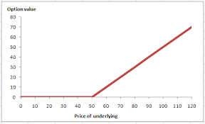
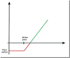
Suppose that the price $S$ of the underlying asset is modeled by a geometric Brownian motion (1.1), and that $r$ is the risk-free rate, assumed to be constant on the period $[0, T]$. One also assumes that there is no dividend on that period. It can be shown [Black and Scholes, 1973] that the value at time $t$, of a European call option of strike price $K$ and maturity $T$, depends only on $S(t)=$ $s$ and on the volatility $\sigma$, and is given by
$$
C(t, s)=s \mathcal{N}\left(d_{1}\right)-K e^{-r(T-t)} \mathcal{N}\left(d_{2}\right)
$$
where $\mathcal{N}^{5}$ is the distribution function of a standard Gaussian variable, and
$$
\begin{aligned}
&d_{1}=\frac{\ln (s / K)+r \tau+\sigma^{2} \tau / 2}{\sigma \sqrt{\tau}} \
&d_{2}=d_{1}-\sigma \sqrt{\tau}=\frac{\ln (s / K)+r \tau-\sigma^{2} \tau / 2}{\sigma \sqrt{\tau}}
\end{aligned}
$$
where $\tau=T-t$ is the time to maturity. Note that as $t \rightarrow T, \tau \rightarrow 0$, and one can check that $\lim _{t \rightarrow T} C(t, s)=\max (s-K, 0)$. Furthermore, as expected, $C(t, s) / s \rightarrow 0$, as $s \rightarrow 0$, and $C(t, s) / s \rightarrow 1$, as $s \rightarrow \infty$ Remark 1.5.1 It is remarkable that the value of the option does not depend on the average return $\mu$, only on the volatility $\sigma$. It does not mean however that $\mu$ is not important. For example, if one wants to characterize the behavior (mean, variance, $V a R$, etc.) of the future value at time $t$ of a portfolio containing call options based on asset $S$, one needs to consider $C{t, S(t)}$, which in turn depends on both parameters $\mu$ and $\sigma$.

金融代写|金融工程作业代写Financial Engineering代考|Estimation Errors

金融工程代写

金融代写|金融工程作业代写Financial Engineering代考|Estimation Errors

一旦计算了最大似然估计,我们应该关注估计误差的性质,即找到

的渐近行为n(μ^n−μ)和n(σ^n−σ). 一般来说,极限分布是多元高斯分布(见附录 A.6.18)。

下一个命题来自附录 B.5.1 的结果。为了表示“法律趋同”,我们使用符号⇝,如附录 B 中所定义。

命题 1.4.1 作为n倾向于∞,(n(μ^n−μ) n(σ^n−σ))收敛到具有协方差矩阵的居中双变量高斯分布在, 表示
(n(μ^n−μ) n(σ^n−σ))⇝ñ2(0,在),
在哪里在=σ22(2H+σ2σ σ1). 一致的估计在是(谁)给的
在^=σ^n22(2H+σ^n2σ^n σ^n1).
特别是,我们得到n(μ^n−μ)/在^11⇝ñ(0,1)和n(σ^n− σ)/在^22↔ñ(0,1).
证明在附录 1.C.2 中给出。

金融代写|金融工程作业代写Financial Engineering代考|Estimation of Parameters for Apple

有关先前结果的应用示例,请考虑 MATLAB 文件 ApplePrices3包含从 1 月开始在纳斯达克 (aapl) 的苹果股票调整后的价值13th ,2009, 一月14th ,2011.

参数估计的结果μ和σ每年的时间尺度,如表 1.1 所示。它们是通过 MATLAB 函数 EstBS1dExp 获得的,使用 Propositions 中的结果1.3.1和 1.4.1。根据我们在第 1.2.2 节末尾对时间尺度和交易日的评论,我们采取了H=1/252.

备注 1.4.1 当使用类似的转换时σ=经验⁡(一种)为了使用不受约束的参数,我们获得了一个估计在0参数估计误差的极限协方差矩阵θ=(μ,一种). 从 delta 方法(定理 B.3.4.1)得出,估计在参数估计误差的极限协方差矩阵(μ,σ)是
在^=Ĵ^在0Ĵ^,  在哪里 Ĵ^=诊断⁡(1,σ^n), IE, Ĵ^=(10 0σ^n). 这是因为 (μ,σ)=

H(μ,一种)=(μ,和一种), 所以雅可比矩阵H是Ĵ=(10 0σ), 估计为Ĵ^.

这种方法在 MATLAB 函数 EstBS1dNum 中实现。有关参数变换和相应的限制协方差矩阵的更多详细信息,请参见备注 B.3.3。

金融代写|金融工程作业代写Financial Engineering代考|European Call Option

假设价格小号标的资产由几何布朗运动 (1.1) 建模,并且r是无风险利率,假设在该周期内保持不变[0,吨]. 人们还假设该期间没有股息。可以证明 [Black and Scholes, 1973]吨, 执行价格的欧式看涨期权ķ和成熟吨, 仅取决于小号(吨)= s以及波动性σ,并且由下式给出
C(吨,s)=sñ(d1)−ķ和−r(吨−吨)ñ(d2)
在哪里ñ5是标准高斯变量的分布函数,并且
d1=ln⁡(s/ķ)+rτ+σ2τ/2στ d2=d1−στ=ln⁡(s/ķ)+rτ−σ2τ/2στ
在哪里τ=吨−吨是成熟的时间。请注意,作为吨→吨,τ→0,并且可以检查林吨→吨C(吨,s)=最大限度(s−ķ,0). 此外,正如预期的那样,C(吨,s)/s→0, 作为s→0, 和C(吨,s)/s→1, 作为s→∞备注 1.5.1 值得注意的是,期权的价值不取决于平均收益μ, 仅关于波动率σ. 然而,这并不意味着μ并不重要。例如,如果要描述行为(均值、方差、在一种R等)的未来价值在时间吨包含基于资产的看涨期权的投资组合小号, 需要考虑C吨,小号(吨), 这又取决于两个参数μ和σ.

金融代写|金融工程作业代写Financial Engineering代考 请认准statistics-lab™

统计代写请认准statistics-lab™. statistics-lab™为您的留学生涯保驾护航。

金融工程代写

金融工程是使用数学技术来解决金融问题。金融工程使用计算机科学、统计学、经济学和应用数学领域的工具和知识来解决当前的金融问题,以及设计新的和创新的金融产品。

非参数统计代写

非参数统计指的是一种统计方法,其中不假设数据来自于由少数参数决定的规定模型;这种模型的例子包括正态分布模型和线性回归模型。

广义线性模型代考

广义线性模型(GLM)归属统计学领域,是一种应用灵活的线性回归模型。该模型允许因变量的偏差分布有除了正态分布之外的其它分布。

术语 广义线性模型(GLM)通常是指给定连续和/或分类预测因素的连续响应变量的常规线性回归模型。它包括多元线性回归,以及方差分析和方差分析(仅含固定效应)。

有限元方法代写

有限元方法(FEM)是一种流行的方法,用于数值解决工程和数学建模中出现的微分方程。典型的问题领域包括结构分析、传热、流体流动、质量运输和电磁势等传统领域。

有限元是一种通用的数值方法,用于解决两个或三个空间变量的偏微分方程(即一些边界值问题)。为了解决一个问题,有限元将一个大系统细分为更小、更简单的部分,称为有限元。这是通过在空间维度上的特定空间离散化来实现的,它是通过构建对象的网格来实现的:用于求解的数值域,它有有限数量的点。边界值问题的有限元方法表述最终导致一个代数方程组。该方法在域上对未知函数进行逼近。[1] 然后将模拟这些有限元的简单方程组合成一个更大的方程系统,以模拟整个问题。然后,有限元通过变化微积分使相关的误差函数最小化来逼近一个解决方案。

tatistics-lab作为专业的留学生服务机构,多年来已为美国、英国、加拿大、澳洲等留学热门地的学生提供专业的学术服务,包括但不限于Essay代写,Assignment代写,Dissertation代写,Report代写,小组作业代写,Proposal代写,Paper代写,Presentation代写,计算机作业代写,论文修改和润色,网课代做,exam代考等等。写作范围涵盖高中,本科,研究生等海外留学全阶段,辐射金融,经济学,会计学,审计学,管理学等全球99%专业科目。写作团队既有专业英语母语作者,也有海外名校硕博留学生,每位写作老师都拥有过硬的语言能力,专业的学科背景和学术写作经验。我们承诺100%原创,100%专业,100%准时,100%满意。

随机分析代写


随机微积分是数学的一个分支,对随机过程进行操作。它允许为随机过程的积分定义一个关于随机过程的一致的积分理论。这个领域是由日本数学家伊藤清在第二次世界大战期间创建并开始的。

时间序列分析代写

随机过程,是依赖于参数的一组随机变量的全体,参数通常是时间。 随机变量是随机现象的数量表现,其时间序列是一组按照时间发生先后顺序进行排列的数据点序列。通常一组时间序列的时间间隔为一恒定值(如1秒,5分钟,12小时,7天,1年),因此时间序列可以作为离散时间数据进行分析处理。研究时间序列数据的意义在于现实中,往往需要研究某个事物其随时间发展变化的规律。这就需要通过研究该事物过去发展的历史记录,以得到其自身发展的规律。

回归分析代写

多元回归分析渐进(Multiple Regression Analysis Asymptotics)属于计量经济学领域,主要是一种数学上的统计分析方法,可以分析复杂情况下各影响因素的数学关系,在自然科学、社会和经济学等多个领域内应用广泛。

MATLAB代写

MATLAB 是一种用于技术计算的高性能语言。它将计算、可视化和编程集成在一个易于使用的环境中,其中问题和解决方案以熟悉的数学符号表示。典型用途包括:数学和计算算法开发建模、仿真和原型制作数据分析、探索和可视化科学和工程图形应用程序开发,包括图形用户界面构建MATLAB 是一个交互式系统,其基本数据元素是一个不需要维度的数组。这使您可以解决许多技术计算问题,尤其是那些具有矩阵和向量公式的问题,而只需用 C 或 Fortran 等标量非交互式语言编写程序所需的时间的一小部分。MATLAB 名称代表矩阵实验室。MATLAB 最初的编写目的是提供对由 LINPACK 和 EISPACK 项目开发的矩阵软件的轻松访问,这两个项目共同代表了矩阵计算软件的最新技术。MATLAB 经过多年的发展,得到了许多用户的投入。在大学环境中,它是数学、工程和科学入门和高级课程的标准教学工具。在工业领域,MATLAB 是高效研究、开发和分析的首选工具。MATLAB 具有一系列称为工具箱的特定于应用程序的解决方案。对于大多数 MATLAB 用户来说非常重要,工具箱允许您学习应用专业技术。工具箱是 MATLAB 函数(M 文件)的综合集合,可扩展 MATLAB 环境以解决特定类别的问题。可用工具箱的领域包括信号处理、控制系统、神经网络、模糊逻辑、小波、仿真等。

R语言代写问卷设计与分析代写
PYTHON代写回归分析与线性模型代写
MATLAB代写方差分析与试验设计代写
STATA代写机器学习/统计学习代写
SPSS代写计量经济学代写
EVIEWS代写时间序列分析代写
EXCEL代写深度学习代写
SQL代写各种数据建模与可视化代写

金融代写|金融工程作业代写Financial Engineering代考| Joint Distribution of Returns

如果你也在 怎样代写金融工程Financial Engineering这个学科遇到相关的难题,请随时右上角联系我们的24/7代写客服。

金融工程是使用数学技术来解决金融问题。金融工程使用计算机科学、统计学、经济学和应用数学领域的工具和知识来解决当前的金融问题,以及设计新的和创新的金融产品。

statistics-lab™ 为您的留学生涯保驾护航 在代写金融工程Financial Engineering方面已经树立了自己的口碑, 保证靠谱, 高质且原创的统计Statistics代写服务。我们的专家在代写金融工程Financial Engineering代写方面经验极为丰富,各种代写金融工程Financial Engineering相关的作业也就用不着说。

我们提供的金融工程Financial Engineering及其相关学科的代写,服务范围广, 其中包括但不限于:

  • Statistical Inference 统计推断
  • Statistical Computing 统计计算
  • Advanced Probability Theory 高等概率论
  • Advanced Mathematical Statistics 高等数理统计学
  • (Generalized) Linear Models 广义线性模型
  • Statistical Machine Learning 统计机器学习
  • Longitudinal Data Analysis 纵向数据分析
  • Foundations of Data Science 数据科学基础
Tag: Continuous Time Markov Chain | WeiYa's Work Yard
金融代写|金融工程作业代写Financial Engineering代考| Joint Distribution of Returns

金融代写|金融工程作业代写Financial Engineering代考|Joint Distribution of Returns

Proposition 1.2.1 Under the Black-Scholes model, for $h>0$ given, the returns $X_{i}=\ln {S(i h)}-\ln [S{(i-1) h}], i \in{1, \ldots, n}$, are independent and $X_{i} \sim N\left(\mu h-\frac{\sigma^{2}}{2} h, \sigma^{2} h\right)$, i.e., $X_{i}$ has a Gaussian distribution with mean $\left(\mu-\frac{\sigma^{2}}{2}\right) h$ and variance $\sigma^{2} h$.
PROOF. For $i \in{1, \ldots, n}$, one has
$$
\begin{aligned}
S(i h) / S{(i-1) h} &=\frac{s e^{\mu i h-\frac{i h \sigma^{2}}{2}}+\sigma W(i h)}{s e^{\mu(i-1) h-\frac{(i-1) h \sigma^{2}}{2}+\sigma W{(i-1) h}}} \
&=e^{\mu h-\frac{h \sigma^{2}}{2}+\sigma{W(i h)-W{(i-1) h}}}
\end{aligned}
$$
so
$$
\begin{aligned}
X_{i} &=\ln [S(i h) / S{(i-1) h}] \
&=\mu h-\frac{\sigma^{2}}{2} h+\sigma{W(i h)-W{(i-1) h}} \
& \sim N\left(\mu h-\frac{\sigma^{2}}{2} h, \sigma^{2} h\right)
\end{aligned}
$$
The increments $W(i h)-W{(i-1) h}, i \in{1 \ldots n}$, being independent, by definition of Brownian motion, it follows that the returns $X_{i}, i \in{1 \ldots n}$, are also independent.

Remark 1.2.2 Since $\sigma$ appears to be a measure of variability, it is also called volatility in financial applications and it is often reported in percentage. For example, a volatility of $20 \%$ per annum means that $\sigma=0.2$, on an annual time scale.

金融代写|金融工程作业代写Financial Engineering代考|Joint Law of Prices

One of the most efficient method for estimating parameters is the maximum likelihood principle, described in Appendix B.1. As shown in Remark B.1.2, the maximum likelihood principle can be used with prices or returns. Since the returns are independent and identically distributed in the BlackScholes model, we will estimate the parameters using the returns instead of the prices.

However, for sake of completeness, we also give the conditional law of the prices, together with their joint law.

Proposition 1.2.2 The conditional distribution of $S{(i+1) h}$, given $S(0)=$ $s, \ldots, S(i h)=s_{i}$, depends only on $S(i h)$, and its density is
$$
f_{S{(i+1) h} \mid S(i h)}\left(x \mid s_{i}\right)=\frac{e^{-\frac{1}{2 \sigma^{2} h}\left{\ln \left(x / s_{i}\right)-\left(\mu-\sigma^{2} / 2\right) h\right}^{2}}}{x \sigma \sqrt{2 \pi h}} \mathbb{I}(x>0), \quad x \in \mathbb{R} .
$$
PROOF. It follows from Proposition $1.2 .1$ that for all $i \geq 0, S{(i+1) h}=$ $S(i h) e^{X_{i+1}}$, and $S(i h)=s e^{X_{1}+\cdots+X_{i}}$ is independent of $e^{X_{i+1}}$. Therefore, the conditional distribution of $S{(i+1) h}$ given $S(0)=s_{0}, \ldots, S(i h)=s_{i}$, is a log-normal distribution (see A.6.8), being the exponential of a Gaussian variate with mean $\ln \left(s_{i}\right)+\left(\mu-\sigma^{2} / 2\right) h$ and variance $\sigma^{2} h$.

Remark 1.2.3 As a by-product of Proposition 1.2.2 and the multiplication formula (A.19), the joint law of $S(h), \ldots, S(n h)$, given $S(0)=s$, is
$$
\begin{aligned}
f_{S(h), \ldots, S(n h) \mid S(0)}\left(s_{1}, \ldots, s_{n} \mid s\right) &=\prod_{i=1}^{n} f_{S((i h) \mid S(0), \ldots, S((i-1) h)}\left(s_{i} \mid s, \ldots, s_{i-1}\right) \
&=\prod_{i=1}^{n} f_{S(i h) \mid S((i-1) h)}\left(s_{i} \mid s_{i-1}\right) \
&=\prod_{i=1}^{n} \frac{e^{-\frac{\left(\ln \left(x_{i}\right)-\ln \left(x_{i-1}\right)-\left(\mu-\sigma^{2} / 2\right)^{h}\right)^{2}}{2 \sigma^{2} h}}}{s_{i} \sqrt{2 \pi \sigma^{2} h}}
\end{aligned}
$$

金融代写|金融工程作业代写Financial Engineering代考|Estimation of Parameters

The maximum likelihood principle described in Appendix B.1 will now be used to estimate parameters $\mu$ and $\sigma$, using the returns as the observations. Usually this method of estimation is more precise than any other one. Since the data are Gaussian, the method of moments, described in Appendix B.8, could also be used. However these two methods yield different results in general.

Recall that the original data set are the prices $S(0)=s_{0}, S(h)=$ $s_{1}, \ldots, S(n h)=s_{n}$, from which we compute the returns $x_{i}=\ln \left(s_{i}\right)-\ln \left(s_{i-1}\right)$, $i \in{1, \ldots, n} .$

Proposition 1.3.1 The estimations of $\mu$ and $\sigma$, obtained by the maximum likelihood principle, are given by
$$
\begin{aligned}
\hat{\mu}{n} &=\frac{\bar{x}}{h}+\frac{s{x}^{2}}{2 h}, \
\hat{\sigma}{n} &=\frac{s{x}}{\sqrt{h}}
\end{aligned}
$$
where $\bar{x}=\frac{1}{n} \sum_{i=1}^{n} x_{i}$ and $s_{x}^{2}=\frac{1}{n} \sum_{i=1}^{n}\left(x_{i}-\bar{x}\right)^{2}$.
The proof is given in Appendix 1.C.1.
Remark 1.3.1 In practice, $\sigma^{2}$ is estimated by
$$
\frac{1}{(n-1) h} \sum_{i=1}^{n}\left(x_{i}-\bar{x}\right)^{2}
$$
the reason being that this estimator is unbiased, while being also quite close to $\frac{s^{2}}{h}$. For example, with MATLAB, the function std $(x)$ returns
$$
\sqrt{\frac{1}{n-1} \sum_{i=1}^{n}\left(x_{i}-\bar{x}\right)^{2}}
$$
instead of
$$
\sqrt{\frac{1}{n} \sum_{i=1}^{n}\left(x_{i}-\bar{x}\right)^{2}}
$$
Remark 1.3.2 When parameters are estimated using the maximum likelihood principle and the observations are not Gaussian, one rarely finds explicit expressions for the estimators. Therefore, one has to use numerical algorithms to maximize the likelihood. In this case, domain constraints on the parameters must be taken into account. For example, in the Black-Scholes model, $\sigma>0$. One can easily replace this sign constraint by setting $\sigma=e^{\alpha}$, with $\alpha \in \mathbb{R}$.

IJFS | Free Full-Text | On Transaction-Cost Models in Continuous-Time  Markets
金融代写|金融工程作业代写Financial Engineering代考| Joint Distribution of Returns

金融工程代写

金融代写|金融工程作业代写Financial Engineering代考|Joint Distribution of Returns

命题 1.2.1 在 Black-Scholes 模型下,对于H>0给定,回报X一世=ln⁡小号(一世H)−ln⁡[小号(一世−1)H],一世∈1,…,n, 是独立的并且X一世∼ñ(μH−σ22H,σ2H), IE,X一世具有均值的高斯分布(μ−σ22)H和方差σ2H.
证明。为了一世∈1,…,n, 一个有
小号(一世H)/小号(一世−1)H=s和μ一世H−一世Hσ22+σ在(一世H)s和μ(一世−1)H−(一世−1)Hσ22+σ在(一世−1)H =和μH−Hσ22+σ在(一世H)−在(一世−1)H
所以
X一世=ln⁡[小号(一世H)/小号(一世−1)H] =μH−σ22H+σ在(一世H)−在(一世−1)H ∼ñ(μH−σ22H,σ2H)
增量在(一世H)−在(一世−1)H,一世∈1…n, 是独立的, 根据布朗运动的定义, 回报X一世,一世∈1…n, 也是独立的。

备注 1.2.2 自σ似乎是一种可变性的度量,它也被称为金融应用中的波动性,通常以百分比报告。例如,波动率20%每年意味着σ=0.2, 在每年的时间尺度上。

金融代写|金融工程作业代写Financial Engineering代考|Joint Law of Prices

估计参数的最有效方法之一是附录 B.1 中描述的最大似然原则。如备注 B.1.2 所示,最大似然原则可用于价格或收益。由于在 BlackScholes 模型中收益是独立且同分布的,我们将使用收益而不是价格来估计参数。

但是,为了完整起见,我们也给出了价格的条件规律,以及它们的联合规律。

命题 1.2.2 的条件分布小号(一世+1)H, 给定小号(0)= s,…,小号(一世H)=s一世, 仅取决于小号(一世H), 其密度为
f_{S{(i+1) h} \mid S(i h)}\left(x \mid s_{i}\right)=\frac{e^{-\frac{1}{2 \sigma^{ 2} h}\left{\ln \left(x / s_{i}\right)-\left(\mu-\sigma^{2} / 2\right) h\right}^{2}}}{ x \sigma \sqrt{2 \pi h}} \mathbb{I}(x>0), \quad x \in \mathbb{R} 。f_{S{(i+1) h} \mid S(i h)}\left(x \mid s_{i}\right)=\frac{e^{-\frac{1}{2 \sigma^{ 2} h}\left{\ln \left(x / s_{i}\right)-\left(\mu-\sigma^{2} / 2\right) h\right}^{2}}}{ x \sigma \sqrt{2 \pi h}} \mathbb{I}(x>0), \quad x \in \mathbb{R} 。
证明。它遵循命题1.2.1为所有人一世≥0,小号(一世+1)H= 小号(一世H)和X一世+1, 和小号(一世H)=s和X1+⋯+X一世独立于和X一世+1. 因此,条件分布小号(一世+1)H给定小号(0)=s0,…,小号(一世H)=s一世, 是对数正态分布(见 A.6.8),是具有均值的高斯变量的指数ln⁡(s一世)+(μ−σ2/2)H和方差σ2H.

备注 1.2.3 作为命题 1.2.2 和乘法公式 (A.19) 的副产品,联合定律小号(H),…,小号(nH), 给定小号(0)=s, 是
F小号(H),…,小号(nH)∣小号(0)(s1,…,sn∣s)=∏一世=1nF小号((一世H)∣小号(0),…,小号((一世−1)H)(s一世∣s,…,s一世−1) =∏一世=1nF小号(一世H)∣小号((一世−1)H)(s一世∣s一世−1) =∏一世=1n和−(ln⁡(X一世)−ln⁡(X一世−1)−(μ−σ2/2)H)22σ2Hs一世2圆周率σ2H

金融代写|金融工程作业代写Financial Engineering代考|Estimation of Parameters

现在将使用附录 B.1 中描述的最大似然原理来估计参数μ和σ,使用回报作为观察。通常这种估计方法比任何其他方法都更精确。由于数据是高斯数据,因此也可以使用附录 B.8 中描述的矩量法。然而,这两种方法通常会产生不同的结果。

回想一下,原始数据集是价格小号(0)=s0,小号(H)= s1,…,小号(nH)=sn, 我们从中计算回报X一世=ln⁡(s一世)−ln⁡(s一世−1), 一世∈1,…,n.

命题 1.3.1 的估计μ和σ,通过最大似然原理获得,由下式给出
μ^n=X¯H+sX22H, σ^n=sXH
在哪里X¯=1n∑一世=1nX一世和sX2=1n∑一世=1n(X一世−X¯)2.
证明在附录 1.C.1 中给出。
备注 1.3.1 在实践中,σ2估计为
1(n−1)H∑一世=1n(X一世−X¯)2
原因是这个估计量是无偏的,同时也非常接近s2H. 例如,对于 MATLAB,函数 std(X)返回
1n−1∑一世=1n(X一世−X¯)2
代替
1n∑一世=1n(X一世−X¯)2
备注 1.3.2 当使用最大似然原理估计参数并且观测值不是高斯分布时,很少会找到估计量的明确表达式。因此,必须使用数值算法来最大化可能性。在这种情况下,必须考虑参数的域约束。例如,在 Black-Scholes 模型中,σ>0. 可以通过设置轻松替换此符号约束σ=和一种, 和一种∈R.

金融代写|金融工程作业代写Financial Engineering代考 请认准statistics-lab™

统计代写请认准statistics-lab™. statistics-lab™为您的留学生涯保驾护航。

金融工程代写

金融工程是使用数学技术来解决金融问题。金融工程使用计算机科学、统计学、经济学和应用数学领域的工具和知识来解决当前的金融问题,以及设计新的和创新的金融产品。

非参数统计代写

非参数统计指的是一种统计方法,其中不假设数据来自于由少数参数决定的规定模型;这种模型的例子包括正态分布模型和线性回归模型。

广义线性模型代考

广义线性模型(GLM)归属统计学领域,是一种应用灵活的线性回归模型。该模型允许因变量的偏差分布有除了正态分布之外的其它分布。

术语 广义线性模型(GLM)通常是指给定连续和/或分类预测因素的连续响应变量的常规线性回归模型。它包括多元线性回归,以及方差分析和方差分析(仅含固定效应)。

有限元方法代写

有限元方法(FEM)是一种流行的方法,用于数值解决工程和数学建模中出现的微分方程。典型的问题领域包括结构分析、传热、流体流动、质量运输和电磁势等传统领域。

有限元是一种通用的数值方法,用于解决两个或三个空间变量的偏微分方程(即一些边界值问题)。为了解决一个问题,有限元将一个大系统细分为更小、更简单的部分,称为有限元。这是通过在空间维度上的特定空间离散化来实现的,它是通过构建对象的网格来实现的:用于求解的数值域,它有有限数量的点。边界值问题的有限元方法表述最终导致一个代数方程组。该方法在域上对未知函数进行逼近。[1] 然后将模拟这些有限元的简单方程组合成一个更大的方程系统,以模拟整个问题。然后,有限元通过变化微积分使相关的误差函数最小化来逼近一个解决方案。

tatistics-lab作为专业的留学生服务机构,多年来已为美国、英国、加拿大、澳洲等留学热门地的学生提供专业的学术服务,包括但不限于Essay代写,Assignment代写,Dissertation代写,Report代写,小组作业代写,Proposal代写,Paper代写,Presentation代写,计算机作业代写,论文修改和润色,网课代做,exam代考等等。写作范围涵盖高中,本科,研究生等海外留学全阶段,辐射金融,经济学,会计学,审计学,管理学等全球99%专业科目。写作团队既有专业英语母语作者,也有海外名校硕博留学生,每位写作老师都拥有过硬的语言能力,专业的学科背景和学术写作经验。我们承诺100%原创,100%专业,100%准时,100%满意。

随机分析代写


随机微积分是数学的一个分支,对随机过程进行操作。它允许为随机过程的积分定义一个关于随机过程的一致的积分理论。这个领域是由日本数学家伊藤清在第二次世界大战期间创建并开始的。

时间序列分析代写

随机过程,是依赖于参数的一组随机变量的全体,参数通常是时间。 随机变量是随机现象的数量表现,其时间序列是一组按照时间发生先后顺序进行排列的数据点序列。通常一组时间序列的时间间隔为一恒定值(如1秒,5分钟,12小时,7天,1年),因此时间序列可以作为离散时间数据进行分析处理。研究时间序列数据的意义在于现实中,往往需要研究某个事物其随时间发展变化的规律。这就需要通过研究该事物过去发展的历史记录,以得到其自身发展的规律。

回归分析代写

多元回归分析渐进(Multiple Regression Analysis Asymptotics)属于计量经济学领域,主要是一种数学上的统计分析方法,可以分析复杂情况下各影响因素的数学关系,在自然科学、社会和经济学等多个领域内应用广泛。

MATLAB代写

MATLAB 是一种用于技术计算的高性能语言。它将计算、可视化和编程集成在一个易于使用的环境中,其中问题和解决方案以熟悉的数学符号表示。典型用途包括:数学和计算算法开发建模、仿真和原型制作数据分析、探索和可视化科学和工程图形应用程序开发,包括图形用户界面构建MATLAB 是一个交互式系统,其基本数据元素是一个不需要维度的数组。这使您可以解决许多技术计算问题,尤其是那些具有矩阵和向量公式的问题,而只需用 C 或 Fortran 等标量非交互式语言编写程序所需的时间的一小部分。MATLAB 名称代表矩阵实验室。MATLAB 最初的编写目的是提供对由 LINPACK 和 EISPACK 项目开发的矩阵软件的轻松访问,这两个项目共同代表了矩阵计算软件的最新技术。MATLAB 经过多年的发展,得到了许多用户的投入。在大学环境中,它是数学、工程和科学入门和高级课程的标准教学工具。在工业领域,MATLAB 是高效研究、开发和分析的首选工具。MATLAB 具有一系列称为工具箱的特定于应用程序的解决方案。对于大多数 MATLAB 用户来说非常重要,工具箱允许您学习应用专业技术。工具箱是 MATLAB 函数(M 文件)的综合集合,可扩展 MATLAB 环境以解决特定类别的问题。可用工具箱的领域包括信号处理、控制系统、神经网络、模糊逻辑、小波、仿真等。

R语言代写问卷设计与分析代写
PYTHON代写回归分析与线性模型代写
MATLAB代写方差分析与试验设计代写
STATA代写机器学习/统计学习代写
SPSS代写计量经济学代写
EVIEWS代写时间序列分析代写
EXCEL代写深度学习代写
SQL代写各种数据建模与可视化代写

金融代写|金融工程作业代写Financial Engineering代考|Black-Scholes Model

如果你也在 怎样代写金融工程Financial Engineering这个学科遇到相关的难题,请随时右上角联系我们的24/7代写客服。

金融工程是使用数学技术来解决金融问题。金融工程使用计算机科学、统计学、经济学和应用数学领域的工具和知识来解决当前的金融问题,以及设计新的和创新的金融产品。

statistics-lab™ 为您的留学生涯保驾护航 在代写金融工程Financial Engineering方面已经树立了自己的口碑, 保证靠谱, 高质且原创的统计Statistics代写服务。我们的专家在代写金融工程Financial Engineering代写方面经验极为丰富,各种代写金融工程Financial Engineering相关的作业也就用不着说。

我们提供的金融工程Financial Engineering及其相关学科的代写,服务范围广, 其中包括但不限于:

  • Statistical Inference 统计推断
  • Statistical Computing 统计计算
  • Advanced Probability Theory 高等概率论
  • Advanced Mathematical Statistics 高等数理统计学
  • (Generalized) Linear Models 广义线性模型
  • Statistical Machine Learning 统计机器学习
  • Longitudinal Data Analysis 纵向数据分析
  • Foundations of Data Science 数据科学基础
A comparison of continuous and discrete time modeling of affective  processes in terms of predictive accuracy | Scientific Reports
金融代写|金融工程作业代写Financial Engineering代考|Black-Scholes Model

金融代写|金融工程作业代写Financial Engineering代考|The Black-Scholes Model

In Black and Scholes [1973], the authors introduced their famous model for the price of a stock, together with a partial differential equation for the value of a European option. To do so, they assumed the following “ideal conditions” on the market:

  • The short-term interest rate, also called risk-free rate, is known and constant until the maturity of the option.
  • The log-returns of the stock follows a Brownian motion with drift.
  • The option is European, i.e., it can only be exercised at maturity.
  • There are no transaction costs, nor penalties for short selling.
  • It is possible to buy or borrow any fraction of the security.
    To make things simpler, we assume that the market is liquid and frictionless, that trading can be done in continuous time, and that the risk-free rate is constant during the life of the option. The latter hypothesis will be weakened in Chapter $3 .$

金融代写|金融工程作业代写Financial Engineering代考|Stock Exchange Data

What do we do when there are dividends or stock splits? In each case, there is a predictable but abnormal jump in the prices. In order to make historical data comparable, it is necessary to take these jumps into account.

For example, in the case of Apple, there were two $2: 1$ stock splits (June $21^{s t}, 2000$, and February $\left.28^{t h}, 2005\right)$, while the last dividend was reported on November $21^{s t}, 1995 .$

In many textbooks on Financial Engineering, e.g., Hull [2006] and Wilmott $[2006]$, it is suggested to replace the stock price $S_{i}$ at the ex-dividend period $i$ by $S_{i}+D_{i}$, where $D_{i}$ is the dividend. In fact, it is often more convenient to do just the opposite ${ }^{1}$, by subtracting the dividend from the pre-dividend price, i.e., the adjusted price for period $i-1$ is $S_{i-1}-D_{i}=S_{i-1} f_{i}$, with $f_{i}=$ $1-D_{i} / S_{i-1}$. In fact, all pre-dividend values $S_{j}, j<i$, are then multiplied by the same factor $f_{i}$. For splits, one proceeds in a similar way. For example, in the case of a 2:1 stock split, all pre-split prices are multiplied by 0.5. The returns are then calculated from these adjusted closing prices. This is in accordance to the standards of the Center for Research in Security Prices (CRSP). The same method is applied to the adjusted prices available on YAHOO!FINANCE website.

金融代写|金融工程作业代写Financial Engineering代考|Continuous Time Models

Let $S(t)$ be the (adjusted) value of an asset at time $t$. Before defining the Black-Scholes model, one needs to define what is a Brownian motion.

Definition 1.2.1 A stochastic process $W$ is a Brownian motion ${ }^{2}$ if it is a

continuous Gaussian process starting at 0 , with zero expectation and covariance function
$$
\operatorname{Cov}{W(s), W(t)}=\min (s, t), s, t \geq 0 .
$$
In particular, if $0=t_{0} \leq t_{1} \leq \cdots \leq t_{n}$, then the increments $W\left(t_{i}\right)-$ $W\left(t_{i-1}\right)$ are independent, have a Gaussian distribution with mean 0 and variance $t_{i}-t_{i-1}, i \in{1, \ldots, n}$.

Definition 1.2.2 (Black-Scholes Model) In the Black-Scholes model, one assumes that the value $S$ of the underlying asset is modeled by a geometric Brownian motion, i.e.,
$$
S(t)=s e^{\left(\mu-\frac{\alpha^{2}}{2}\right) t+\sigma W(t)}, \quad t \geq 0,
$$
where $W$ is a Brownian motion.
Note that $S$ is often defined as the solution to the following stochastic differential equation:
$$
d S(t)=\mu S(t) d t+\sigma S(t) d W(t), S(0)=s .
$$
Remark 1.2.1 The Black-Scholes model depends on two unknown parameters: $\mu$ and $\sigma$. Therefore they must be estimated. In practice, data are collected at regular time intervals of given length $h$. For example, observations can be collected every 5 seconds, daily, weekly, monthly, etc.

It is also important to characterize the parameters. For example, is $\mu$ an expectation? If so, it is the expectation of which variable? One can ask the same question for the parameter $\sigma$.

In what follows, we will see that $\mu$ and $\sigma$ can be interpreted in terms of the log-returns
$$
X_{i}=X_{i}(h)=\ln {S(i h)}-\ln [S{(i-1) h}], \quad i \in{1, \ldots, n} .
$$
First, we need to find the joint law of these returns. In addition to being important for the estimation of the unknown parameters, the distribution of the returns is needed in order to find expressions for option prices or when using Monte Carlo methods for pricing complex options, measuring risk or performance, etc.

金融代写|金融工程作业代写Financial Engineering代考|Black-Scholes Model

金融工程代写

金融代写|金融工程作业代写Financial Engineering代考|The Black-Scholes Model

在 Black 和 Scholes [1973] 中,作者介绍了他们著名的股票价格模型,以及欧式期权价值的偏微分方程。为此,他们假设了市场上的以下“理想条件”:

  • 短期利率,也称为无风险利率,在期权到期之前是已知的并且是恒定的。
  • 股票的对数收益遵循带有漂移的布朗运动。
  • 期权是欧式的,即只能在到期时行使。
  • 没有交易成本,也没有卖空的处罚。
  • 可以购买或借入任何部分的证券。
    为简单起见,我们假设市场是流动的且无摩擦的,交易可以在连续的时间内完成,并且在期权的生命周期内无风险利率是恒定的。后一种假设将在本章中被削弱3.

金融代写|金融工程作业代写Financial Engineering代考|Stock Exchange Data

当有股息或股票分割时,我们该怎么办?在每种情况下,价格都会出现可预测但异常的上涨。为了使历史数据具有可比性,有必要考虑这些跳跃。

例如,在 Apple 的案例中,有两个2:1股票分割(六月21s吨,2000, 二月28吨H,2005),而最后一次股息是在 11 月报告的21s吨,1995.

在许多金融工程教科书中,例如 Hull [2006] 和 Wilmott[2006], 建议更换股价小号一世在除息期一世经过小号一世+D一世, 在哪里D一世是股息。事实上,做相反的事情往往更方便1,通过从股息前的价格中减去股息,即期间的调整价格一世−1是小号一世−1−D一世=小号一世−1F一世, 和F一世= 1−D一世/小号一世−1. 事实上,所有的股息前值小号j,j<一世, 然后乘以相同的因子F一世. 对于拆分,以类似的方式进行。例如,在 2:1 股票分割的情况下,所有分割前的价格都乘以 0.5。然后根据这些调整后的收盘价计算回报。这符合证券价格研究中心 (CRSP) 的标准。同样的方法也适用于雅虎财经网站上的调整价格。

金融代写|金融工程作业代写Financial Engineering代考|Continuous Time Models

让小号(吨)是当时资产的(调整后的)价值吨. 在定义 Black-Scholes 模型之前,需要定义什么是布朗运动。

定义 1.2.1 随机过程在是布朗运动2如果它是一个

从 0 开始的连续高斯过程,期望和协方差函数为零
这⁡在(s),在(吨)=分钟(s,吨),s,吨≥0.
特别是,如果0=吨0≤吨1≤⋯≤吨n,那么增量在(吨一世)− 在(吨一世−1)是独立的,具有均值为 0 和方差的高斯分布吨一世−吨一世−1,一世∈1,…,n.

定义 1.2.2(Black-Scholes 模型) 在 Black-Scholes 模型中,假设值小号标的资产由几何布朗运动建模,即
小号(吨)=s和(μ−一种22)吨+σ在(吨),吨≥0,
在哪里在是布朗运动。
注意小号通常定义为以下随机微分方程的解:
d小号(吨)=μ小号(吨)d吨+σ小号(吨)d在(吨),小号(0)=s.
备注 1.2.1 Black-Scholes 模型取决于两个未知参数:μ和σ. 因此必须对它们进行估计。在实践中,以给定长度的固定时间间隔收集数据H. 例如,可以每 5 秒、每天、每周、每月等收集一次观察结果。

表征参数也很重要。例如,是μ期望?如果是,是哪个变量的期望值?可以对参数提出相同的问题σ.

在接下来的内容中,我们将看到μ和σ可以根据日志返回来解释
X一世=X一世(H)=ln⁡小号(一世H)−ln⁡[小号(一世−1)H],一世∈1,…,n.
首先,我们需要找到这些回报的联合规律。除了对未知参数的估计很重要外,还需要收益分布来找到期权价格的表达式,或者在使用蒙特卡罗方法对复杂期权进行定价、衡量风险或绩效等时。

金融代写|金融工程作业代写Financial Engineering代考 请认准statistics-lab™

统计代写请认准statistics-lab™. statistics-lab™为您的留学生涯保驾护航。

金融工程代写

金融工程是使用数学技术来解决金融问题。金融工程使用计算机科学、统计学、经济学和应用数学领域的工具和知识来解决当前的金融问题,以及设计新的和创新的金融产品。

非参数统计代写

非参数统计指的是一种统计方法,其中不假设数据来自于由少数参数决定的规定模型;这种模型的例子包括正态分布模型和线性回归模型。

广义线性模型代考

广义线性模型(GLM)归属统计学领域,是一种应用灵活的线性回归模型。该模型允许因变量的偏差分布有除了正态分布之外的其它分布。

术语 广义线性模型(GLM)通常是指给定连续和/或分类预测因素的连续响应变量的常规线性回归模型。它包括多元线性回归,以及方差分析和方差分析(仅含固定效应)。

有限元方法代写

有限元方法(FEM)是一种流行的方法,用于数值解决工程和数学建模中出现的微分方程。典型的问题领域包括结构分析、传热、流体流动、质量运输和电磁势等传统领域。

有限元是一种通用的数值方法,用于解决两个或三个空间变量的偏微分方程(即一些边界值问题)。为了解决一个问题,有限元将一个大系统细分为更小、更简单的部分,称为有限元。这是通过在空间维度上的特定空间离散化来实现的,它是通过构建对象的网格来实现的:用于求解的数值域,它有有限数量的点。边界值问题的有限元方法表述最终导致一个代数方程组。该方法在域上对未知函数进行逼近。[1] 然后将模拟这些有限元的简单方程组合成一个更大的方程系统,以模拟整个问题。然后,有限元通过变化微积分使相关的误差函数最小化来逼近一个解决方案。

tatistics-lab作为专业的留学生服务机构,多年来已为美国、英国、加拿大、澳洲等留学热门地的学生提供专业的学术服务,包括但不限于Essay代写,Assignment代写,Dissertation代写,Report代写,小组作业代写,Proposal代写,Paper代写,Presentation代写,计算机作业代写,论文修改和润色,网课代做,exam代考等等。写作范围涵盖高中,本科,研究生等海外留学全阶段,辐射金融,经济学,会计学,审计学,管理学等全球99%专业科目。写作团队既有专业英语母语作者,也有海外名校硕博留学生,每位写作老师都拥有过硬的语言能力,专业的学科背景和学术写作经验。我们承诺100%原创,100%专业,100%准时,100%满意。

随机分析代写


随机微积分是数学的一个分支,对随机过程进行操作。它允许为随机过程的积分定义一个关于随机过程的一致的积分理论。这个领域是由日本数学家伊藤清在第二次世界大战期间创建并开始的。

时间序列分析代写

随机过程,是依赖于参数的一组随机变量的全体,参数通常是时间。 随机变量是随机现象的数量表现,其时间序列是一组按照时间发生先后顺序进行排列的数据点序列。通常一组时间序列的时间间隔为一恒定值(如1秒,5分钟,12小时,7天,1年),因此时间序列可以作为离散时间数据进行分析处理。研究时间序列数据的意义在于现实中,往往需要研究某个事物其随时间发展变化的规律。这就需要通过研究该事物过去发展的历史记录,以得到其自身发展的规律。

回归分析代写

多元回归分析渐进(Multiple Regression Analysis Asymptotics)属于计量经济学领域,主要是一种数学上的统计分析方法,可以分析复杂情况下各影响因素的数学关系,在自然科学、社会和经济学等多个领域内应用广泛。

MATLAB代写

MATLAB 是一种用于技术计算的高性能语言。它将计算、可视化和编程集成在一个易于使用的环境中,其中问题和解决方案以熟悉的数学符号表示。典型用途包括:数学和计算算法开发建模、仿真和原型制作数据分析、探索和可视化科学和工程图形应用程序开发,包括图形用户界面构建MATLAB 是一个交互式系统,其基本数据元素是一个不需要维度的数组。这使您可以解决许多技术计算问题,尤其是那些具有矩阵和向量公式的问题,而只需用 C 或 Fortran 等标量非交互式语言编写程序所需的时间的一小部分。MATLAB 名称代表矩阵实验室。MATLAB 最初的编写目的是提供对由 LINPACK 和 EISPACK 项目开发的矩阵软件的轻松访问,这两个项目共同代表了矩阵计算软件的最新技术。MATLAB 经过多年的发展,得到了许多用户的投入。在大学环境中,它是数学、工程和科学入门和高级课程的标准教学工具。在工业领域,MATLAB 是高效研究、开发和分析的首选工具。MATLAB 具有一系列称为工具箱的特定于应用程序的解决方案。对于大多数 MATLAB 用户来说非常重要,工具箱允许您学习应用专业技术。工具箱是 MATLAB 函数(M 文件)的综合集合,可扩展 MATLAB 环境以解决特定类别的问题。可用工具箱的领域包括信号处理、控制系统、神经网络、模糊逻辑、小波、仿真等。

R语言代写问卷设计与分析代写
PYTHON代写回归分析与线性模型代写
MATLAB代写方差分析与试验设计代写
STATA代写机器学习/统计学习代写
SPSS代写计量经济学代写
EVIEWS代写时间序列分析代写
EXCEL代写深度学习代写
SQL代写各种数据建模与可视化代写