风险建模代写

分类：风险建模代写

统计代写|风险建模代写Financial risk modeling代考|News effects on the exchange rate

Posted on 2022年5月4日2022年5月4日 by statistics-lab

如果你也在怎样代写风险建模Financial risk modeling这个学科遇到相关的难题，请随时右上角联系我们的24/7代写客服。

风险建模是确定有多少风险存在于一个特定的企业、投资或一系列的现金流中。

statistics-lab™ 为您的留学生涯保驾护航在代写风险建模Financial risk modeling方面已经树立了自己的口碑, 保证靠谱, 高质且原创的统计Statistics代写服务。我们的专家在代写风险建模Financial risk modeling代写方面经验极为丰富，各种代写风险建模Financial risk modeling相关的作业也就用不着说。

我们提供的风险建模Financial risk modeling及其相关学科的代写，服务范围广, 其中包括但不限于:

Statistical Inference 统计推断
Statistical Computing 统计计算
Advanced Probability Theory 高等楖率论
Advanced Mathematical Statistics 高等数理统计学
(Generalized) Linear Models 广义线性模型
Statistical Machine Learning 统计机器学习
Longitudinal Data Analysis 纵向数据分析
Foundations of Data Science 数据科学基础

统计代写|风险建模代写Financial risk modeling代考|News effects on the exchange rate

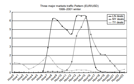
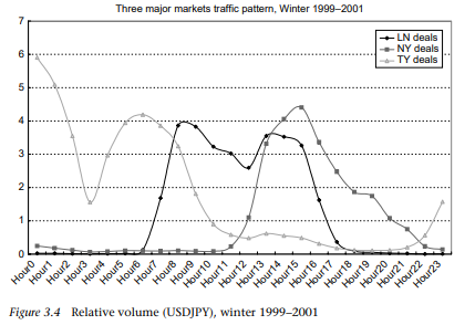
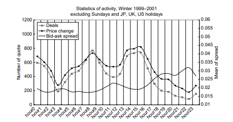
As shown in the previous section, transaction volume tends to surge during a particular time of the day. One of the reasons for a surge in transactions is a concentrated arrival of new macro information in the markets. The possible existence of private information may cause a different trading response by dealers, some of them informed and some uninformed, to the arrival of new information. Then the trading may be intensified between these two types of dealers, as described in the “private information model” of Easley and O’Hara (1992).

In this section, the exchange rate reaction to the release of major macroeconomic statistics is examined. In particular, this section examines how the dollar/yen exchange rate market digests information contained in the various macroeconomic statistics’ releases – to what extent transactions and prices react to the macroeconomic statistics’ news, how long the news effect lasts and which news has the most/least impact on the exchange rate. In the analysis, the unexpected component of macroeconomic announcements, a “surprise,” is defined by the difference between the actual indicator announcement and the average of predicted indicators by the market. The sample period is from 2001 to 2005 and we examine the impacts from 12 Japanese macroeconomic statistics’ releases on the exchange rate returns, volatility and the transaction volume.

统计代写|风险建模代写Financial risk modeling代考|Japanese macroeconomic announcements

Chaboud et al. (2004) study the impact of US macroeconomic announcements on exchange rates using the following US macro variables: payroll, GDP advanced, PPI, retail sales, trade balance and Fed funds rate (target). These authors found a significant impact on exchange rate returns from a surprise component in the announcement. In the European perspective, Ehrmann and Fratzscher (2005) used GDP, Ifo business climate index, business confidence balance, PPI, CPI, retail sales, trade balance, M3, unemployment, industrial production and manufacturing orders as proxies for Germany news releases. 22

In contrast to US macroeconomic announcements, most of which come out at $8.30 \mathrm{am}$ (EST), the release time of Japanese news announcements varies from news to news. Some of the announcements are released in the morning and others in the afternoon. Most of the major macroeconomic statistics come out at either $8.30 \mathrm{am}, 8.50 \mathrm{am}, 10.30 \mathrm{am}$, $2.00 \mathrm{pm}$ or $2.30 \mathrm{pm}$.

After 2001, the announcement time for Japanese macroeconomic statistics has become fairly standardized. Until 2000 , however, a lot of news was released one hour earlier than the current release time, while some news releases were fixed later or went back and forth. For example, the current CPI release time was set at $8.30$ only in 2002 . Release time of three news announcements (balance of payments [8:50], trade balance [8:50] and retail sales [14:30]) changed once in early 2000 and moved back to the original time about six months later.

Figures $3.6$ and $3.7$ show the average of number of deals on newsrelease days and non-announcement days for Tankan (Bank of Japan, business survey) and GDP preliminary (GDPP, at $8.50 \mathrm{am}$ JST). This announcement time is just before the first peak in transactions within the day and, therefore, this surge of activity may likely reflect the impact of news releases. ${ }^{23}$ Each figure plots the 15 -minute averages in the number of transactions from 6 am to 12 noon for 2001-2005. The red line shows the benchmark of no macro announcement, and the black line shows the deal activity on announcement days. The top panel of the figure shows the difference in the number of deals between news-announcement days and non-announcement days.

统计代写|风险建模代写Financial risk modeling代考|Impact of surprises on exchange rate activities

When an announcement has unexpected content the announcement is expected to be followed by a change in the exchange rate, because market participants react to this unexpected part by rebalancing their portfolio positions. That is, a surprise would result in changes – positively or negatively – in the exchange rate returns through changes in the number of deals. The release of a news announcement itself, regardless of surprises, may affect price volatility. Suppose that the actual announcement of a macro announcement is exactly the same as the average of market expectations. Then there should not be any positive or negative returns that follow the announcement of no surprise. However, even if the “average” expectation is confirmed by the actual announcement, individuals may be heterogeneous and some are positively surprised and some negatively surprised. Hence, those who were off the average have incentives to trade and price volatility may rise with returns being zero. The total amount of deals may increase at the time of macroeconomic announcement. Unless market participants are homogeneous in expectations on the news – which is very unlikely – some deals are bound to occur right after the announcement. When there is a surprise component in the news, additional deal activities will be stimulated.

Hashimoto and Ito (2009) examined whether and how much an unexpected component of a macroeconomic news announcement, a “surprise, ” will affect returns, volatility and the number of transactions in the dollar/yen exchange market with the following estimations: ${ }^{24}$ Return regression:
$$
\begin{aligned}
\Delta s(t, u) &=\sum_{i(u)=1}^{n(u)} \alpha_{i(u)} N_{i(u)}(t, u)+\varepsilon(t, u) \
\Delta s(t, u) &=\sum_{i(u)=1}^{n(u)} \alpha_{i(u)} N_{i(u)}(t, u)+\delta \Delta s(t, u-k)+\theta N D(t, u-k)+\varepsilon(t, u)
\end{aligned}
$$

统计代写|风险建模代写Financial risk modeling代考|News effects on the exchange rate

如上一节所示，交易量往往会在一天中的特定时间激增。交易激增的原因之一是新宏观信息集中涌入市场。私人信息的可能存在可能会导致交易商对新信息的到来产生不同的交易反应，其中一些是知情的，一些是不知情的。然后，这两种类型的经销商之间的交易可能会加剧，如 Easley 和 O’Hara（1992）的“私人信息模型”中所述。

在本节中，研究了主要宏观经济统计数据发布后的汇率反应。特别是，本节研究美元/日元汇率市场如何消化各种宏观经济统计数据发布中包含的信息——交易和价格对宏观经济统计数据新闻的反应程度、新闻效应持续多长时间以及哪些新闻具有对汇率的影响最大/最小。在分析中，宏观经济公告的意外成分，即“意外”，定义为实际指标公告与市场预测指标平均值之间的差异。样本期为 2001 年至 2005 年，我们考察了 12 项日本宏观经济统计数据发布对汇率回报、波动性和交易量的影响。

统计代写|风险建模代写Financial risk modeling代考|Japanese macroeconomic announcements

查布德等人。（2004 年）使用以下美国宏观变量研究美国宏观经济公告对汇率的影响：工资、GDP 增长、PPI、零售额、贸易差额和联邦基金利率（目标）。这些作者发现公告中的一个意外部分对汇率回报产生了重大影响。从欧洲的角度来看，Ehrmann 和 Fratzscher (2005) 使用 GDP、Ifo 商业景气指数、商业信心平衡、PPI、CPI、零售销售、贸易平衡、M3、失业率、工业生产和制造业订单作为德国新闻发布的代理。22

与美国宏观经济公告相反，其中大部分发布于8.30一种米（EST），日本新闻公告的发布时间因新闻而异。有些公告在上午发布，有些则在下午发布。大多数主要的宏观经济统计数据都是在8.30一种米,8.50一种米,10.30一种米, 2.00p米或者2.30p米.

2001年以后，日本宏观经济统计数据的公布时间已经相当规范。然而，直到 2000 年，很多新闻都比当前发布时间提前了一个小时发布，而一些新闻发布则更晚一些，或者来回走动。例如，当前 CPI 发布时间设置为8.30仅在 2002 年。三个新闻公告（国际收支[8:50]、贸易平衡[8:50]和零售[14:30]）的发布时间在2000年初改变了一次，大约六个月后又回到了原来的时间。

数据3.6和3.7显示短观（日本银行，商业调查）和 GDP 初步（GDPP，at8.50一种米JST）。该公告时间正好在当天交易的第一个高峰之前，因此，这种活动激增可能反映了新闻发布的影响。23每个图都绘制了 2001-2005 年从早上 6 点到中午 12 点的 15 分钟平均交易次数。红线表示没有宏观公告的基准，黑线表示公告日的交易活动。该图的顶部显示了新闻公告日和非公告日之间交易数量的差异。

统计代写|风险建模代写Financial risk modeling代考|Impact of surprises on exchange rate activities

当公告包含意外内容时，预计该公告之后会出现汇率变化，因为市场参与者通过重新平衡其投资组合头寸来应对这一意外部分。也就是说，意外将通过交易数量的变化导致汇率回报发生积极或消极的变化。新闻公告本身的发布，无论是否意外，都可能影响价格波动。假设宏观公告的实际公告与市场预期的平均值完全相同。那么在毫无意外的宣布之后不应该有任何正或负的回报。然而，即使“平均”预期得到实际公告的证实，个人可能是异质的，有些人感到惊讶，有些人感到惊讶。因此，那些偏离平均水平的人有交易动机，价格波动可能会随着回报为零而上升。在宏观经济公布时，交易总量可能会增加。除非市场参与者对新闻的预期一致——这是非常不可能的——否则一些交易肯定会在宣布后立即发生。当新闻中有惊喜成分时，会刺激额外的交易活动。除非市场参与者对新闻的预期一致——这是非常不可能的——否则一些交易肯定会在宣布后立即发生。当新闻中有惊喜成分时，会刺激额外的交易活动。除非市场参与者对消息的预期一致——这是非常不可能的——否则一些交易肯定会在消息发布后立即发生。当新闻中有惊喜成分时，会刺激额外的交易活动。

Hashimoto 和 Ito (2009) 研究了宏观经济新闻公告中的意外组成部分，即“意外”，是否以及在多大程度上会影响美元/日元交易市场的回报、波动性和交易数量，并做出以下估计：24返回回归：
Δs(吨,在)=∑一世(在)=1n(在)一种一世(在)ñ一世(在)(吨,在)+e(吨,在) Δs(吨,在)=∑一世(在)=1n(在)一种一世(在)ñ一世(在)(吨,在)+dΔs(吨,在−ķ)+θñD(吨,在−ķ)+e(吨,在)

统计代写|风险建模代写Financial risk modeling代考|Intraday patterns

Posted on 2022年5月4日2022年5月4日 by statistics-lab

如果你也在怎样代写风险建模Financial risk modeling这个学科遇到相关的难题，请随时右上角联系我们的24/7代写客服。

风险建模是确定有多少风险存在于一个特定的企业、投资或一系列的现金流中。

我们提供的风险建模Financial risk modeling及其相关学科的代写，服务范围广, 其中包括但不限于:

Statistical Inference 统计推断
Statistical Computing 统计计算
Advanced Probability Theory 高等楖率论
Advanced Mathematical Statistics 高等数理统计学
(Generalized) Linear Models 广义线性模型
Statistical Machine Learning 统计机器学习
Longitudinal Data Analysis 纵向数据分析
Foundations of Data Science 数据科学基础

统计代写|风险建模代写Financial risk modeling代考|Intraday patterns

统计代写|风险建模代写Financial risk modeling代考|Activities during a day

The intraday patterns of foreign exchange transaction are anecdotally and instinctively known to bank dealers. However, only a few academic papers have statistically examined market activities so far. Ito and Hashimoto $(2004,2006)$ were one of the first teams to analyze the foreign exchange market using tick-by-tick deal data.

Following Ito and Hashimoto (2006), this section examines highfrequency data on foreign exchange market activities such as the “number of quotes,” the “number of deals,” “bid-ask spread” and the “relative volume share” in order to show the intraday patterns of the foreign exchange market. The sample period is from 1999 to 2001 . The number of quotes is calculated as the number of seconds where quotes are recorded, and the number of deals is the sum of bid-side deals and askside deals in each hour of the day. 12 The “relative volume” is defined as

hourly aggregated relative volumes: the percentage share of transaction volume in one minute relative to the total transaction volume in one day. The hourly transaction volumes, with each contract (transaction) being one million of the “base currency” (the first currency in the currency pair name), are divided by the total trading volume of the day. ${ }^{13}$ These indicators of market activities are calculated for one hour and then averaged over three years with a differentiation of the standard and daylight saving time. 14

Figure $3.2$ shows the intraday (Hour $0-23$ ) patterns of the numbers of deals, quotes and the bid-ask spread of the USDJPY and Figure $3.3$ shows those of the EURUSD. 15

统计代写|风险建模代写Financial risk modeling代考|Regional contribution

The above analysis based on counts of deals and quotes reveals that the transaction activities become exceptionally high during the overlapping business hours of the currency pair home markets – the Tokyo afternoon and London morning (the second peak) and the London afternoon and the US morning (the third peak). The next question is on the regional contribution to the surge in activities. For example, whether a surge in activities in the Tokyo mid-afternoon hours and London morning hours can be attributed to the activity of Tokyo participants or London participants. In the following section, we decompose the regional contributions to the activity surge by the relative trading volume shares which have the label of participants (regional names).

The regional contributions to the surge in trades for dollar/yen activities are shown in Figure $3.4$ and for euro/dollar in Figure $3.5^{17}$ The dollar/yen trades during the overlapping hours of the Tokyo afternoon and London morning are done by Tokyo (and Asian) participants (financial institutions in Japan and Asia region) and London (and European) participants (financial institutions in Europe) around GMT Hours 6-8,

with the majority of Tokyo participants at the beginning and then with the increasing share of London participants. During this time period, transactions from New York (the United States) participants (financial institutions in North America) are quite small and almost negligible. On the other hand, the dollar/yen trades during the overlapping hours of the London afternoon and the New York morning are mainly done by London and New York participants with some Tokyo participants.

The figures also reveal that transactions by Tokyo participants and London participants exhibit a U-shape pattern, whereas the transactions by New York participants have a single-peak pattern. The monotonic decline in market activities, the number of deals and quotes, after the New York afternoon may be due to two reasons: there is no pickup effect in the New York afternoon (unlike the Tokyo or London markets) and the transactions after GMT 16 are mainly done by the New York participants (almost no participants from Tokyo and London). The very large trade volume among the Tokyo participants during the Tokyo business hours (except for lunch hours) implies that, for the dollar/yen trade, the Tokyo market has new information, inducing heterogeneous reactions to the news, thereby generating more trade.

统计代写|风险建模代写Financial risk modeling代考|Market opening hours

As seen in the analysis above, each market experiences a surge in transactions during the opening hours. When there are many participants in the market (the market is “deep”), trading volume tends to be higher and spreads tend to be narrower. The opening hour of the Tokyo market appears to have special characteristics because it follows a few hours of extremely low activity after the New York market closes. In particular, the Monday morning of the Tokyo market probably has some specific activity patterns because the Tokyo market is the first to open after a long weekend break, from Friday night to Monday morning. The first hour of Tokyo on Monday (Hour 0 in adjusted GMT) may be different because the volume of orders accumulated during the weekend (about 35 hours) is much larger than those accumulated during the overnight gap (2-3 hours between the New York close and Tokyo opening) resulting in much higher activity compared to the same hour on any other day of the week. Similarly, we expect the opening hours of the London and New York markets to show some special characteristics in trading activity.

Ito and Hashimoto (2006) examined the opening-hour effect of the three markets (Tokyo, London and New York), the Monday morning effect and the (lack of) U-shape pattern by testing the significance of dummy variables that take the value 1 when deals/quotes are recorded in the opening hours (or Monday opening hours). They found that, in general, the negative relationship between the number of deals (quotes) and the spread holds even for these opening hours. That is, when the market is deep (when the number of price [quotes] changes is large) the bid-ask spread tends to be narrower.

The Tokyo opening effect and Tokyo Monday opening effect are tested by examining the relationship between the spread and the number of deals/quotes with opening-hour dummies. 18 For the Tokyo opening effect in 1999 , it turns out that the spread becomes narrower as the number of deals/quotes increases during the opening hour, 9 am Tokyo time, for both the dollar/yen trade and the euro/dollar trade. On the other hand, as for the Monday opening effect, it is found that the number of deals significantly increases during the Monday opening hours for the dollar/yen trade in 1999 and 2000 , suggesting that the market participants carry out some orders accumulated over the weekend in the first hour of the week, the Monday Tokyo morning at GMT Hour 0 , despite the relatively wide bid-ask spread. The Monday Tokyo effect is not found for the euro/dollar trade.

风险建模代写

统计代写|风险建模代写Financial risk modeling代考|Activities during a day

外汇交易的日内模式对于银行交易商来说是轶事和本能地知道的。然而，到目前为止，只有少数学术论文对市场活动进行了统计研究。伊藤和桥本(2004,2006)是最早使用逐笔交易数据分析外汇市场的团队之一。

继 Ito 和 Hashimoto（2006 年）之后，本节研究了外汇市场活动的高频数据，例如“报价数量”、“交易数量”、“买卖价差”和“相对交易量份额”，以便显示外汇市场的盘中格局。样本期为 1999 年至 2001 年。报价数量计算为记录报价的秒数，成交数量是一天中每个小时的买入方成交和卖出方成交的总和。12 “相对体积”定义为

每小时总相对交易量：一分钟的交易量相对于一天的总交易量的百分比。每小时交易量，每份合约（交易）为一百万“基础货币”（货币对名称中的第一个货币），除以当天的总交易量。13这些市场活动指标按一小时计算，然后在三年内取平均值，区分标准时间和夏令时。14

数字3.2显示盘中（小时0−23) 交易数量、报价和 USDJPY 的买卖差价的模式和图3.3显示 EURUSD 的那些。15

统计代写|风险建模代写Financial risk modeling代考|Regional contribution

上述基于成交和报价统计的分析表明，在货币对国内市场重叠营业时间——东京下午和伦敦上午（第二个高峰）以及伦敦下午和美国上午（第三高峰）。下一个问题是区域对活动激增的贡献。例如，东京午后时间和伦敦上午时间的活动激增是否可以归因于东京参与者或伦敦参与者的活动。在下一节中，我们将区域对活动激增的贡献分解为具有参与者（区域名称）标签的相对交易量份额。

区域对美元/日元活动交易激增的贡献如图所示3.4以及图中的欧元/美元3.517东京下午和伦敦上午重叠时段的美元/日元交易由东京（和亚洲）参与者（日本和亚洲地区的金融机构）和伦敦（和欧洲）参与者（欧洲的金融机构）在格林威治标准时间前后进行6-8,

一开始是东京的大多数参与者，然后是伦敦参与者的比例越来越高。在此期间，来自纽约（美国）参与者（北美金融机构）的交易非常小，几乎可以忽略不计。另一方面，伦敦下午和纽约上午重叠时段的美元/日元交易主要由伦敦和纽约参与者以及一些东京参与者完成。

数据还显示，东京参与者和伦敦参与者的交易呈现 U 形模式，而纽约参与者的交易呈现单峰模式。纽约下午之后市场活动、成交和报价数量单调下降可能是由于两个原因：纽约下午没有回升效应（与东京或伦敦市场不同）以及 GMT 16 之后的交易主要由纽约参与者完成（东京和伦敦几乎没有参与者）。在东京营业时间（午餐时间除外），东京参与者之间的巨大交易量意味着，对于美元/日元的交易，东京市场有新的信息，引起对新闻的不同反应，从而产生更多的交易。

统计代写|风险建模代写Financial risk modeling代考|Market opening hours

从上面的分析可以看出，每个市场在开放时间内的交易量都会激增。当市场参与者众多时（市场“深度”），交易量往往会更高，点差往往会更窄。东京市场的开市时间似乎具有特殊性，因为它是在纽约市场收盘后几个小时的极低活动之后。尤其是东京市场的周一早上可能有一些特定的活动模式，因为东京市场是在从周五晚上到周一早上的长周末休息后最先开市的。周一东京的第一个小时（调整后的格林威治标准时间为 0 小时）可能会有所不同，因为周末（约 35 小时）累积的订单量远大于隔夜间隔期间（纽约之间的 2-3 小时）累积的订单量关闭和东京开放）与一周中任何其他一天的同一小时相比，活动量要高得多。同样，我们预计伦敦和纽约市场的开市时间将在交易活动中表现出一些特殊特征。

Ito 和 Hashimoto（2006 年）通过检验取值的虚拟变量的显着性，检验了三个市场（东京、伦敦和纽约）的开市时间效应、周一早上效应和（缺乏）U 形模式1 当交易/报价记录在营业时间（或周一营业时间）时。他们发现，一般来说，交易数量（报价）与价差之间的负相关关系即使在这些开放时间也成立。也就是说，当市场深度时（当价格 [报价] 变化的数量很大时），买卖差价往往会更窄。

东京开盘效应和东京星期一开盘效应通过检查价差与开盘时间虚拟交易/报价数量之间的关系来测试。18 对于 1999 年的东京开市效应，事实证明，在东京时间上午 9 点的开市时间，无论是美元/日元交易还是欧元/美元交易，价差都随着交易/报价数量的增加而变窄。另一方面，关于周一开盘效应，发现1999年和2000年的美元/日元交易在周一开盘时间内成交数量明显增加，表明市场参与者进行了一些累积的订单。周末在一周的第一个小时，即周一东京早上 GMT 0 时，尽管买卖价差相对较大。

统计代写|风险建模代写Financial risk modeling代考|Market Microstructure of the Foreign Exchange Markets

Posted on 2022年5月4日2022年5月4日 by statistics-lab

如果你也在怎样代写风险建模Financial risk modeling这个学科遇到相关的难题，请随时右上角联系我们的24/7代写客服。

风险建模是确定有多少风险存在于一个特定的企业、投资或一系列的现金流中。

我们提供的风险建模Financial risk modeling及其相关学科的代写，服务范围广, 其中包括但不限于:

Statistical Inference 统计推断
Statistical Computing 统计计算
Advanced Probability Theory 高等楖率论
Advanced Mathematical Statistics 高等数理统计学
(Generalized) Linear Models 广义线性模型
Statistical Machine Learning 统计机器学习
Longitudinal Data Analysis 纵向数据分析
Foundations of Data Science 数据科学基础

Competition: Wind-dependent Variables: Predict Wind Speeds of Tropical Storms — 统计代写|风险建模代写Financial risk modeling代考|Market Microstructure of the Foreign Exchange Markets

统计代写|风险建模代写Financial risk modeling代考|Evidence from the Electronic Broking System

The foreign exchange market remains sleepless. In contrast to stock exchange markets which are subject to strict opening and closing times each day and where transactions are done in a specific space (such as the New York Stock Exchange and Tokyo Stock Exchange), someone is trading somewhere all the time $-24$ hours a day, (almost) 7 days a week in foreign exchange markets.

The state of the global foreign exchange market is clarified by a market survey conducted by central banks under coordination of the Bank for International Settlements (BIS) once every three years. The most recent survey was conducted in April 2007 and the BIS report was issued in 2007. According to the survey, as shown in Table 3.1, following a brief decline between 1998 and 2001, the average daily turnover of the foreign exchange steadily increased after 2001 reaching $\$ 1.8$ trl in 2004 followed by the record high of $\$ 3.1$ trl in $2007.1$ Of the turnover in 2007 , spot transactions accounted for $\$ 1005$ billion, ${ }^{2}$ outright forward $\$ 361$ for billion and swaps $\$ 1714$ billion. Decomposing into currencies, approximately 43 percent of transactions are in US dollars, 18 percent are in euros, 8 percent in Japanese yen, 7 percent in pound sterling and 3 percent in Swiss francs. As for the currency pairs, $\$$ /euro accounted for $\$ 840$ bil, $\$ /$ yen for $\$ 397$ bil and \$/GBP for $\$ 361$ bil.

Foreign exchange transactions take place between dealers of reporting financial institutions, between a dealer and another financial institution or between a dealer and a nonfinancial customer. One of the remarkable features is a recent sharp increase in transactions between dealers and other financial institutions, whereas the percentage share of transactions between dealers and between dealers and nonfinancial institutions remains almost constant. The declining share of transactions between dealers who report to the BIS surveys can be partly explained by the grow ing role of electronic brokers in the spot interbank market. 3 This trend means that “hot potatoes” (Lyons, 1997), transmissions of orders by large retail customers to a bank that generate multiplied transactions in the interbank market through a price discovery process, are less important now and a cool supercomputer has become increasingly important.

统计代写|风险建模代写Financial risk modeling代考|Literature review

Conventional wisdom in the academic literature is that the exchange rate follows random walk for frequencies less than annual, for example, daily, weekly or even monthly, whereas it sometimes shows time trends, cyclicality or, in general, history dependence at lower frequencies. While traditional economics textbooks are based on the random-walk hypothesis, financial institutions continue to bet millions of dollars on the predictability of exchange rate movements. The gap between the random walk in academia and the prediction model in the real world is remarkable, but in recent years there has been a growing academic

literature on exchange rate forecasting and empirical investigation using high-frequency data – “market microstructure” analysis. 4

As for predictability and random walk, using high-frequency deal and quote prices of USDJPY and EURUSD exchange rates, Hashimoto et al. (2008) found that deal price movements tend to continue a run once started, whereas quote prices mostly follow a random walk. Ito and Hashimoto (2008) showed by using high-frequency data from the actual trade platform that exchange rates could be predictable at up to five minutes and the predictability disappears after 30 minutes. Evans and Lyons (2005a, 2005b) also examined daily EURUSD exchange rate returns based on the end-user data and found a persistent (days) effect in currency markets.

Some studies focus on whether exchange rates respond to pressures of customers’ orders. Evans and Lyons (2002), for example, reported a positive relation between daily exchange rate returns and order flows for Deutsche mark/dollar. Love and Payne (2003) and Berger et al. (2005) studied the contemporaneous relationship between order flow and the exchange rate. Evans and Lyons (2005c) consider heterogeneity of order flow in estimating its price impact. Based on the end-user order flow data, they show that order flow provides information to market makers. Lyons’ series of papers $(1995,1996,1997,1998,2001)$ developed a theoretical model of order flows and information transmission. In line with the information and pricing in markets, Lyons and Moore (2005) found that exchange rate prices are affected by transactions.

Intraday activities such as the number of deals and transaction volume in foreign exchange markets are also of interest in the market microstructure analysis. Admati and Pfleiderer (1988), Brock and Kleidon (1992) and Hsieh and Kleidon (1996) provided theoretical and empirical backgrounds of intraday patterns of the bid-ask spread and volatility. Baillie and Bollerslev (1990) and Andersen and Bollerslev (1997, 1998) were some of the earliest studies that examined intraday volatility of exchange rates using indicative quotes. Finally, Chaboud et al. (2004), Berger et al. (2005) and Ito and Hashimoto $(2006,2008)$ examine the intraday behavior of exchange rates using up-to-date high-frequency data.

统计代写|风险建模代写Financial risk modeling代考|Data

The spot foreign exchange markets have evolved in recent years and now the overwhelming majority of spot foreign exchange transactions are executed through a global electronic broking systems such as EBS and Reuters D-3000. These electronic broking systems provide trading technology and display quotes and transactions continuously for 24 hours a day. Fifteen years ago brokers in the interbank market were mostly human and direct deals between dealers held a substantial share of the spot market. The foreign exchange market of today is very different. Now, each financial institution that establishes an account with EBS and/or Reuters D-3000 is given a specific computer screen and is able to trade via this screen by putting in and hitting prices. The EBS has a stronger market share in absolute terms than Reuters D-3000 in currencies such as the dollar/yen, euro/dollar, euro/yen, euro/chf etc., and is said to cover more than 90 percent of the dollar/yen and euro/dollar trades. In

contrast, Reuters has significant market share in transactions related to the pound sterling, the Canadian dollar and the Australian dollar.

The EBS data set has advantages over the frequently used indicative quotes of exchange rate data such as the FXFX of Reuters in at least two important aspects. First, the quotes in the EBS data set are “firm,” in that banks that post quotes are committed to trade at those quoted prices, when they are “hit.” . In contrast, the indicative quotes of the FXFX screen are those input by dealers for information only, without any commitment for trade. Indicative quotes are much less reliable than firm quotes in capturing the whole picture of a market reality. Second, transactions’ data available in the EBS data set is simply not available on the FXFX screen. Although exact trading volume is not disclosed, transaction counts (counts of seconds that had at least one transaction) and trade volume shares (a percentage share of trading volumes in one minute) are available in the EBS data set.

As part of facilitating an orderly market, EBS requires any newly linked institution to secure a sufficient number of other banks that are willing to open credit lines with the newcomer. A smaller or a regional bank may have fewer trading relationships, thus not as many credit relationships. Then the best bid and ask for that institution may be different from the best bid and ask of the market. A smaller or regional bank may post more aggressive prices (higher bids or lower asks) because they will have relatively fewer credit relationships, implying that they will see fewer dealable prices generally.

风险建模代写

统计代写|风险建模代写Financial risk modeling代考|Evidence from the Electronic Broking System

外汇市场依然不眠不休。与每天都有严格的开市和收市时间以及在特定空间进行交易的证券交易所市场（例如纽约证券交易所和东京证券交易所）相比，有人一直在某处交易−24每天几个小时，（几乎）每周 7 天在外汇市场上。

由中央银行在国际清算银行 (BIS) 的协调下每三年进行一次的市场调查澄清了全球外汇市场的状况。最近一次调查于 2007 年 4 月进行，BIS 报告于 2007 年发布。根据调查，如表 3.1 所示，外汇日均成交量在经历了 1998 年至 2001 年的短暂下降后，2001 年之后稳步上升到达$1.8trl 在 2004 年之后创下历史新高$3.1输入2007.12007年营业额中，现货交易占$1005十亿，2彻底向前$361十亿和掉期$1714十亿。分解成货币，大约 43% 的交易是美元，18% 是欧元，8% 是日元，7% 是英镑，3% 是瑞士法郎。至于货币对，$/欧元占$840比尔，$/日元$397bil 和$ /GBP 为$361比尔。

外汇交易发生在报告金融机构的交易商之间、交易商与另一家金融机构之间或交易商与非金融客户之间。显着特点之一是近期交易商与其他金融机构之间的交易急剧增加，而交易商之间以及交易商与非金融机构之间的交易百分比几乎保持不变。向 BIS 调查报告的交易商之间的交易份额下降的部分原因是电子经纪人在现货银行同业市场中的作用越来越大。3 这种趋势意味着“烫手山芋”（Lyons，1997 年），大型零售客户向银行传输订单，通过价格发现过程在银行间市场产生成倍的交易，

统计代写|风险建模代写Financial risk modeling代考|Literature review

学术文献中的传统观点是，汇率在低于年度的频率下遵循随机游走，例如，每天、每周甚至每月，而它有时会显示时间趋势、周期性或一般而言，较低频率的历史依赖性。虽然传统经济学教科书基于随机游走假设，但金融机构继续将数百万美元押在汇率变动的可预测性上。学术界的随机游走与现实世界的预测模型之间的差距是显着的，但近年来学术界越来越多

使用高频数据进行汇率预测和实证研究的文献——“市场微观结构”分析。4

至于可预测性和随机游走，使用 USDJPY 和 EURUSD 汇率的高频交易和报价，Hashimoto 等人。(2008) 发现交易价格的变动往往会在开始后继续运行，而报价大多遵循随机游走。Ito 和 Hashimoto（2008）通过使用来自实际贸易平台的高频数据表明，汇率在 5 分钟内可以预测，30 分钟后可预测性消失。Evans 和 Lyons (2005a, 2005b) 还根据最终用户数据检查了每日 EURUSD 汇率回报，并发现货币市场存在持续（天数）效应。

一些研究侧重于汇率是否对客户订单的压力作出反应。例如，Evans 和 Lyons (2002) 报告了每日汇率回报与德国马克/美元订单流之间的正相关关系。Love and Payne (2003) 和 Berger 等人。（2005）研究了订单流和汇率之间的同期关系。Evans 和 Lyons (2005c) 在估计其价格影响时考虑了订单流的异质性。根据最终用户的订单流数据，他们表明订单流为做市商提供了信息。里昂系列论文(1995,1996,1997,1998,2001)建立了订单流和信息传递的理论模型。根据市场的信息和定价，Lyons 和 Moore（2005）发现汇率价格受交易影响。

外汇市场的交易数量和交易量等盘中活动也是市场微观结构分析的重点。Admati 和 Pfleiderer (1988)、Brock 和 Kleidon (1992) 以及 Hsieh 和 Kleidon (1996) 提供了日内买卖价差和波动性模式的理论和经验背景。Baillie 和 Bollerslev (1990) 以及 Andersen 和 Bollerslev (1997, 1998) 是最早使用指示性报价检查汇率日内波动的一些研究。最后，Chaboud 等人。（2004 年），伯杰等人。（2005）和伊藤和桥本(2006,2008)使用最新的高频数据检查汇率的日内表现。

统计代写|风险建模代写Financial risk modeling代考|Data

即期外汇市场近年来发生了变化，现在绝大多数的即期外汇交易是通过 EBS 和 Reuters D-3000 等全球电子经纪系统执行的。这些电子经纪系统提供交易技术，并每天 24 小时连续显示报价和交易。15 年前，银行间市场的经纪人大多是人工交易，交易商之间的直接交易占据了现货市场的很大份额。今天的外汇市场非常不同。现在，每个在 EBS 和/或 Reuters D-3000 建立账户的金融机构都拥有一个特定的计算机屏幕，并且能够通过该屏幕通过输入和击中价格进行交易。EBS在美元/日元、欧元/美元、欧元/日元、欧元/瑞士法郎等货币中的绝对市场份额高于路透社D-3000，据说覆盖了90%以上的美元/日元和欧元/美元交易。在

相比之下，路透社在与英镑、加元和澳元相关的交易中占有相当大的市场份额。

EBS 数据集至少在两个重要方面比路透社的 FXFX 等经常使用的汇率数据指示性报价具有优势。首先，EBS 数据集中的报价是“确定的”，因为发布报价的银行承诺在报价受到“打击”时以这些报价进行交易。. 相比之下，FXFX屏幕的指示性报价是交易商输入的仅供参考的报价，没有任何交易承诺。在捕捉市场现实的全貌方面，指示性报价远不如实盘报价可靠。其次，在 EBS 数据集中可用的交易数据在 FXFX 屏幕上根本不可用。虽然没有透露确切的交易量，

作为促进有序市场的一部分，EBS 要求任何新建立关联的机构确保有足够数量的其他银行愿意向新加入者开设信贷额度。较小的或区域性银行可能有较少的贸易关系，因此没有那么多的信用关系。那么该机构的最佳买入价和卖出价可能与市场的最佳买入价和卖出价不同。较小的或区域性银行可能会发布更激进的价格（更高的出价或更低的要价），因为它们的信用关系相对较少，这意味着它们通常会看到较少的可交易价格。

统计代写|风险建模代写Financial risk modeling代考请认准statistics-lab™

统计代写请认准statistics-lab™. statistics-lab™为您的留学生涯保驾护航。

金融工程代写

金融工程是使用数学技术来解决金融问题。金融工程使用计算机科学、统计学、经济学和应用数学领域的工具和知识来解决当前的金融问题，以及设计新的和创新的金融产品。

非参数统计代写

非参数统计指的是一种统计方法，其中不假设数据来自于由少数参数决定的规定模型；这种模型的例子包括正态分布模型和线性回归模型。

广义线性模型代考

广义线性模型（GLM）归属统计学领域，是一种应用灵活的线性回归模型。该模型允许因变量的偏差分布有除了正态分布之外的其它分布。

术语广义线性模型（GLM）通常是指给定连续和/或分类预测因素的连续响应变量的常规线性回归模型。它包括多元线性回归，以及方差分析和方差分析（仅含固定效应）。

有限元方法代写

有限元方法（FEM）是一种流行的方法，用于数值解决工程和数学建模中出现的微分方程。典型的问题领域包括结构分析、传热、流体流动、质量运输和电磁势等传统领域。

有限元是一种通用的数值方法，用于解决两个或三个空间变量的偏微分方程（即一些边界值问题）。为了解决一个问题，有限元将一个大系统细分为更小、更简单的部分，称为有限元。这是通过在空间维度上的特定空间离散化来实现的，它是通过构建对象的网格来实现的：用于求解的数值域，它有有限数量的点。边界值问题的有限元方法表述最终导致一个代数方程组。该方法在域上对未知函数进行逼近。[1] 然后将模拟这些有限元的简单方程组合成一个更大的方程系统，以模拟整个问题。然后，有限元通过变化微积分使相关的误差函数最小化来逼近一个解决方案。

tatistics-lab作为专业的留学生服务机构，多年来已为美国、英国、加拿大、澳洲等留学热门地的学生提供专业的学术服务，包括但不限于Essay代写，Assignment代写，Dissertation代写，Report代写，小组作业代写，Proposal代写，Paper代写，Presentation代写，计算机作业代写，论文修改和润色，网课代做，exam代考等等。写作范围涵盖高中，本科，研究生等海外留学全阶段，辐射金融，经济学，会计学，审计学，管理学等全球99%专业科目。写作团队既有专业英语母语作者，也有海外名校硕博留学生，每位写作老师都拥有过硬的语言能力，专业的学科背景和学术写作经验。我们承诺100%原创，100%专业，100%准时，100%满意。

随机分析代写

随机微积分是数学的一个分支，对随机过程进行操作。它允许为随机过程的积分定义一个关于随机过程的一致的积分理论。这个领域是由日本数学家伊藤清在第二次世界大战期间创建并开始的。

时间序列分析代写

随机过程，是依赖于参数的一组随机变量的全体，参数通常是时间。随机变量是随机现象的数量表现，其时间序列是一组按照时间发生先后顺序进行排列的数据点序列。通常一组时间序列的时间间隔为一恒定值（如1秒，5分钟，12小时，7天，1年），因此时间序列可以作为离散时间数据进行分析处理。研究时间序列数据的意义在于现实中，往往需要研究某个事物其随时间发展变化的规律。这就需要通过研究该事物过去发展的历史记录，以得到其自身发展的规律。

回归分析代写

多元回归分析渐进（Multiple Regression Analysis Asymptotics）属于计量经济学领域，主要是一种数学上的统计分析方法，可以分析复杂情况下各影响因素的数学关系，在自然科学、社会和经济学等多个领域内应用广泛。

MATLAB代写

MATLAB 是一种用于技术计算的高性能语言。它将计算、可视化和编程集成在一个易于使用的环境中，其中问题和解决方案以熟悉的数学符号表示。典型用途包括：数学和计算算法开发建模、仿真和原型制作数据分析、探索和可视化科学和工程图形应用程序开发，包括图形用户界面构建MATLAB 是一个交互式系统，其基本数据元素是一个不需要维度的数组。这使您可以解决许多技术计算问题，尤其是那些具有矩阵和向量公式的问题，而只需用 C 或 Fortran 等标量非交互式语言编写程序所需的时间的一小部分。MATLAB 名称代表矩阵实验室。MATLAB 最初的编写目的是提供对由 LINPACK 和 EISPACK 项目开发的矩阵软件的轻松访问，这两个项目共同代表了矩阵计算软件的最新技术。MATLAB 经过多年的发展，得到了许多用户的投入。在大学环境中，它是数学、工程和科学入门和高级课程的标准教学工具。在工业领域，MATLAB 是高效研究、开发和分析的首选工具。MATLAB 具有一系列称为工具箱的特定于应用程序的解决方案。对于大多数 MATLAB 用户来说非常重要，工具箱允许您学习和应用专业技术。工具箱是 MATLAB 函数（M 文件）的综合集合，可扩展 MATLAB 环境以解决特定类别的问题。可用工具箱的领域包括信号处理、控制系统、神经网络、模糊逻辑、小波、仿真等。

R语言代写	问卷设计与分析代写
PYTHON代写	回归分析与线性模型代写
MATLAB代写	方差分析与试验设计代写
STATA代写	机器学习/统计学习代写
SPSS代写	计量经济学代写
EVIEWS代写	时间序列分析代写
EXCEL代写	深度学习代写
SQL代写	各种数据建模与可视化代写

统计代写|风险建模代写Financial risk modeling代考| The timeline of a limit order history

Posted on 2022年5月4日2022年5月4日 by statistics-lab

如果你也在怎样代写风险建模Financial risk modeling这个学科遇到相关的难题，请随时右上角联系我们的24/7代写客服。

风险建模是确定有多少风险存在于一个特定的企业、投资或一系列的现金流中。

我们提供的风险建模Financial risk modeling及其相关学科的代写，服务范围广, 其中包括但不限于:

Statistical Inference 统计推断
Statistical Computing 统计计算
Advanced Probability Theory 高等楖率论
Advanced Mathematical Statistics 高等数理统计学
(Generalized) Linear Models 广义线性模型
Statistical Machine Learning 统计机器学习
Longitudinal Data Analysis 纵向数据分析
Foundations of Data Science 数据科学基础

Query Result Size Estimation - ML Wiki — 统计代写|风险建模代写Financial risk modeling代考| The timeline of a limit order history

统计代写|风险建模代写Financial risk modeling代考|The timeline of a limit order history

A stylized timeline of the limit order history is shown on the next page. The first row marks the clock time $T_{i}$ (measured in seconds since start of the trading day), the second row marks the time $t_{k i}$ since the moment $t_{k 0}$ of $k$ th limit order arrival, the third row marks $i(k)$ duration episodes $\Delta t_{k i}$ between consecutive changes of covariates $x_{k i}$ and the fourth row shows the values of time-varying covariates immediately before the beginning of each new episode of the limit order history. Row five shows the hazard rate $v\left(x_{k 0}\right)$ of cancellation for fleeting orders, row six shows the hazard rate $\xi\left(x_{k i}\right)$ of cancellation for regular (non-fleeting) limit orders and row seven shows the hazard rate $\mu\left(\boldsymbol{x}{k i}\right) R\left(\boldsymbol{x}{k i}\right)$ of order execution in each of the durations prior to the $k$ th limit order termination.

统计代写|风险建模代写Financial risk modeling代考|The likelihood function

To derive the expression for the likelihood function $L_{k}$ of $k$ th limit order, we start with the model where the risks of execution and cancellation are conditionally independent given the values of covariates. Then we show how the derived log-likelihood function can be maximized by standard methods of survival analysis, since the likelihood function $L_{k}$ can be decomposed into the product of two terms, $L_{c k}$ and $L_{e k}$, corresponding to the likelihood terms of cancellation and execution risks. The likelihood function of cancellation can be written as follows:
$$
\begin{aligned}
L_{c k}(\pi, v, \xi)=& \frac{e^{-\pi^{\prime} x_{k 0}}}{1+e^{-\pi^{\prime} x_{k 0}}} \exp \left[\sum_{i=1}^{i(k)}\left(\delta_{k i} \ln v\left(x_{k 0}\right)-v\left(x_{k 0}\right) \Delta t_{k i}\right)\right] \
&+\frac{1}{1+e^{-\pi^{\prime} x_{k 0}}} \exp \left[\sum_{i=1}^{i(k)}\left(\delta_{k i} \ln \xi\left(x_{k i}\right)-\xi\left(x_{k i}\right) \Delta t_{k i}\right)\right]
\end{aligned}
$$
where $\delta_{k i}$ is the indicator of the event that ith duration episode is terminated by cancellation. The likelihood function of execution is written similarly as:
$$
L_{e k}(\mu)=\exp \left[\sum_{i=1}^{i(k)}\left(d_{k i} \ln \mu\left(x_{k i}\right)-R\left(x_{k i}\right) \mu\left(x_{k i}\right) \Delta t_{k i}\right)\right]
$$
where $d_{k i}$ is the indicator of the event that ith duration episode is terminated by execution.

The log-likelihood function corresponding to the cancellation risk can be written in the additive form as follows:
$$
\begin{aligned}
\ln L_{c k}(\pi, v, \xi)=&-\left(\pi^{\prime} x_{k 0}+\ln \left(1+e^{-\pi^{\prime} x_{k 0}}\right)+\ln \left(1+Z_{c k}(\pi, v, \xi)\right)\right) \
&+\sum_{i=1}^{i(k)}\left(\delta_{k i} \ln v\left(x_{k 0}\right)-v\left(x_{k 0}\right) \Delta t_{k i}\right)
\end{aligned}
$$
where
$$
Z_{c k}(\pi, v, \xi)=\pi^{\prime} x_{k 0}+\sum_{i=1}^{i(k)}\left(\delta_{k i} y_{k i}-v\left(x_{k 0}\right)\left(1-e^{y_{k i}}\right)\right)
$$
and
$$
y_{k i}=\ln \xi\left(x_{k i}\right)-\ln v\left(x_{k 0}\right) .
$$
The log-likelihood function corresponding to execution risk is written similarly as follows:
$$
\ln L_{e k}(\mu)=\sum_{i=1}^{i(k)}\left(d_{k i} \ln \mu\left(x_{k i}\right)-R\left(x_{k i}\right) \mu\left(x_{k i}\right) \Delta t_{k i}\right)
$$

统计代写|风险建模代写Financial risk modeling代考|Estimation results

Panel A of Table $2.7$ shows the results for the model of intensity of limit order arrival at best quotes for ask orders for 13 randomly chosen stocks and Panel B shows the same for the mixture model for cancellation of limit orders arriving at best quotes. Estimates that have the same sign at least 90 percent of the days are boldfaced.

Panel $B$ shows that the probability of a fleeting order at best ask quotes depends:

positively on bid-ask spread,
positively on recent buyer-initiated trading volume (in the last 5 seconds),
positively (but not as strongly) on recent (last 5 seconds) executions of hidden bid orders,
negatively on LOB depth at and near the best quote on the same side,
negatively (except for ISRG) on LOB depth at best quote on the opposite side,
negatively for small relative spread stocks (AAPL, CMCSA) and positively for larger relative spread stocks (AKAM, GOOG, ISRG) on recent (in the last five seconds) seller-initiated trading volume.

The intensity of limit order arrival at best ask quotes (shown in Panel A)

depends positively on bid-ask spread,
depends positively on recent (in the last five seconds) buyer- and seller-initiated trading volume, although more strongly on sellerinitiated trading volume,
depends negatively on LOB depth at and near the best quote on the opposite side,
exhibits positive dependence on LOB depth near the same side best quote for AMGN and ISRG and negative dependence on LOB depth near the same side best quote for CMCSA.

风险建模代写

统计代写|风险建模代写Financial risk modeling代考|The timeline of a limit order history

限价单历史的程式化时间线显示在下一页。第一行标记时钟时间吨一世（以交易日开始后的秒数为单位），第二行标记时间吨ķ一世从那一刻起吨ķ0的ķ限价单到货，第三排标记一世(ķ)持续时间剧集Δ吨ķ一世在协变量的连续变化之间Xķ一世第四行显示限价单历史的每个新片段开始之前的时变协变量值。第五行显示危险率在(Xķ0)取消转瞬即逝的订单，第 6 行显示危险率X(Xķ一世)常规（非暂时性）限价单的取消，第 7 行显示危险率μ(Xķ一世)R(Xķ一世)在之前的每个持续时间的订单执行ķ限价单终止。

统计代写|风险建模代写Financial risk modeling代考|The likelihood function

导出似然函数的表达式大号ķ的ķ对于限价单，我们从模型开始，其中执行和取消的风险在给定协变量值的情况下是条件独立的。然后我们展示了如何通过标准的生存分析方法最大化导出的对数似然函数，因为似然函数大号ķ可以分解为两项的乘积，大号Cķ和大号和ķ，对应于取消和执行风险的可能性条款。抵消的似然函数可以写成如下：
大号Cķ(圆周率,在,X)=和−圆周率′Xķ01+和−圆周率′Xķ0经验⁡[∑一世=1一世(ķ)(dķ一世ln⁡在(Xķ0)−在(Xķ0)Δ吨ķ一世)] +11+和−圆周率′Xķ0经验⁡[∑一世=1一世(ķ)(dķ一世ln⁡X(Xķ一世)−X(Xķ一世)Δ吨ķ一世)]
在哪里dķ一世是第 i 个持续时间情节因取消而终止的事件的指示符。执行的似然函数类似地写成：
大号和ķ(μ)=经验⁡[∑一世=1一世(ķ)(dķ一世ln⁡μ(Xķ一世)−R(Xķ一世)μ(Xķ一世)Δ吨ķ一世)]
在哪里dķ一世是第 i 个持续时间的情节被执行终止的事件的指标。

取消风险对应的对数似然函数可以写成加法形式如下：
ln⁡大号Cķ(圆周率,在,X)=−(圆周率′Xķ0+ln⁡(1+和−圆周率′Xķ0)+ln⁡(1+从Cķ(圆周率,在,X))) +∑一世=1一世(ķ)(dķ一世ln⁡在(Xķ0)−在(Xķ0)Δ吨ķ一世)
在哪里
从Cķ(圆周率,在,X)=圆周率′Xķ0+∑一世=1一世(ķ)(dķ一世是ķ一世−在(Xķ0)(1−和是ķ一世))
和
是ķ一世=ln⁡X(Xķ一世)−ln⁡在(Xķ0).
执行风险对应的对数似然函数写法类似如下：
ln⁡大号和ķ(μ)=∑一世=1一世(ķ)(dķ一世ln⁡μ(Xķ一世)−R(Xķ一世)μ(Xķ一世)Δ吨ķ一世)

统计代写|风险建模代写Financial risk modeling代考|Estimation results

表 A 面板2.7显示了 13 只随机选择的股票的卖出订单的限价订单到达最佳报价强度模型的结果，面板 B 显示了取消到达最佳报价的限价订单的混合模型的相同结果。至少 90% 的天数具有相同符号的估计值以粗体显示。

控制板乙表明转瞬即逝的订单充其量要价的概率取决于：

积极的买卖差价，
对近期买家发起的交易量（在最后 5 秒内）持积极态度，
对最近（最后 5 秒）隐藏的投标订单执行积极（但不那么强烈），
在同一侧的最佳报价处和附近对 LOB 深度产生负面影响，
负面（ISRG 除外）对 LOB 深度的最佳报价在另一侧，
在最近（过去 5 秒内）卖方发起的交易量中，对相对价差较小的股票（AAPL、CMCSA）不利，对价差较大的股票（AKAM、GOOG、ISRG）有利。

限价单到达最佳卖价的强度（如面板 A 所示）

正依赖于买卖差价，
积极地取决于最近（在最后 5 秒内）买方和卖方发起的交易量，尽管更强烈地取决于卖方发起的交易量，
负面取决于对面最佳报价处和附近的 LOB 深度，
对 AMGN 和 ISRG 的同侧最佳报价附近的 LOB 深度表现出正相关性，对 CMCSA 的同侧最佳报价附近的 LOB 深度表现出负相关性。

统计代写请认准statistics-lab™. statistics-lab™为您的留学生涯保驾护航。

金融工程代写

非参数统计代写

非参数统计指的是一种统计方法，其中不假设数据来自于由少数参数决定的规定模型；这种模型的例子包括正态分布模型和线性回归模型。

广义线性模型代考

广义线性模型（GLM）归属统计学领域，是一种应用灵活的线性回归模型。该模型允许因变量的偏差分布有除了正态分布之外的其它分布。

有限元方法代写

随机分析代写

时间序列分析代写

回归分析代写

MATLAB代写

R语言代写	问卷设计与分析代写
PYTHON代写	回归分析与线性模型代写
MATLAB代写	方差分析与试验设计代写
STATA代写	机器学习/统计学习代写
SPSS代写	计量经济学代写
EVIEWS代写	时间序列分析代写
EXCEL代写	深度学习代写
SQL代写	各种数据建模与可视化代写

统计代写|风险建模代写Financial risk modeling代考|Principal components of execution and cancellation probabilities

Posted on 2022年5月4日2022年5月4日 by statistics-lab

如果你也在怎样代写风险建模Financial risk modeling这个学科遇到相关的难题，请随时右上角联系我们的24/7代写客服。

风险建模是确定有多少风险存在于一个特定的企业、投资或一系列的现金流中。

我们提供的风险建模Financial risk modeling及其相关学科的代写，服务范围广, 其中包括但不限于:

Statistical Inference 统计推断
Statistical Computing 统计计算
Advanced Probability Theory 高等楖率论
Advanced Mathematical Statistics 高等数理统计学
(Generalized) Linear Models 广义线性模型
Statistical Machine Learning 统计机器学习
Longitudinal Data Analysis 纵向数据分析
Foundations of Data Science 数据科学基础

统计代写|风险建模代写Financial risk modeling代考|Principal components of execution and cancellation probabilities

We use the following covariates for our principal components analysis:

Price = the INET average transaction price per share,
Sprd = the INET inside spread,
Range $=$ the five-minute INET price range,
Disvol = the INET share volume from executions against displayed limit orders,
Hinvol = the INET volume of executions against hidden orders inside the INET spread,
Houtvol = the five-minute INET volume from executions against hidden orders on the edges of the INET bid-ask spread,
Dep1 = the average displayed depth of the INET book at the best bid and ask prices,
Dep5 = the average displayed depth of the INET order book at the top five ticks on bid and ask sides of the book, and
Shrs = the number of outstanding common shares for each stock on June $30,2006 .$

Panel A of Table $2.5$ shows the correlation matrix for the above covariates. The majority of these variables have a coefficient of correlation of greater than 50 percent with at least one of the other variables. Given this, we apply principal component analysis to effect a dimension reduction. We extract the first five principal components for the stock-specific averages of our covariates Logprice $=\ln ($ Price $)$, Logsprd $=$ $\ln ($ Sprd-1), Logrange $=\ln ($ Range $), \quad$ Logdisvol $=\ln ($ Disvol $), \quad$ Loghinvol $=$ $\ln ($ Hinvol $), \quad$ Loghoutvol $=\ln ($ Houtvol $), \quad$ Logdep $1=\ln ($ Dep 1$), \quad$ Logdep5 $=$ $\ln ($ Dep5 $)$ and Logshrs $=\ln ($ Shrs $)$. The five principal components $P C 1, \ldots$, $P C S$ are constructed as linear combinations of the above covariates so that they have orthonormal loading coefficients and $P C 1$ is chosen to explain the largest proportion of variation in the covariates, $P C 2$ explains the largest proportion of the variation that is left unexplained by the first component, $P C 3$ explains the largest proportion of variance unexplained by the first two components and so forth. The linear combination coefficients for each principal component are reported in Panel C of Table $2.5$. The first five factors $P C 1, \ldots, P C 5$ are related to our covariates by the

统计代写|风险建模代写Financial risk modeling代考|The mixture of distributions model

We began our analysis by illustrating order cancellation rates for one stock, Comcast (CMCSA) – showing the high rates of cancellation at very short durations, which then taper off as time increases. We then showed that this pattern is robust across stocks. The dynamics of order cancellation at very short durations differ from those at longer time intervals. We use these observations to posit that instead of specifying one distribution to model order cancellations, a better approach would be to formulate a mixture of distributions – one that draws the fleeting orders from one distribution and longer duration orders from another.

统计代写|风险建模代写Financial risk modeling代考|Assumptions and notation

Assume we have access to the complete history of a limit order $k$, which was entered into the limit order book at time $T_{0}$. Prior to the limit order entering the book, the observed covariates capturing the market conditions were at the level $x_{k 0}$. Assume that the first change of the covariates to the new level $x_{k 1}$ occurs at time $T_{1}$, within $t_{k 1}$ seconds since the order arrival; the second change of the covariates to the new level $x_{k 2}$ occurs at time $T_{2}$, within $t_{k 2}$ seconds since this limit order arrival; and so on, until termination of the limit order at time $T_{i(k)}$, within $t_{k i(k)}$ seconds after the order arrival and the covariates prior to the limit order termination stayed at the level $\boldsymbol{x}_{k i(k)}$. Assume there are three possible causes for limit order termination: (1) cancellation, (2) full execution, and (3) censoring. In addition, we may allow for the possibility of partial executions during the lifetime of the limit order.

Upon arrival, the limit order assumes one of the two types: (1) fleeting or (2) regular (non-fleeting). The newly arrived order is fleeting with probability $\pi\left(x_{k 0}\right)=\exp \left(-\pi^{\prime} x_{k 0}\right) /\left(1+\exp \left(-\pi^{\prime} x_{k 0}\right)\right)$ and non-fleeting with the complementary probability $1 /\left(1+\exp \left(-\pi^{\prime} x_{k 0}\right)\right)$. If the order is fleeting then the risk of its cancellation depends on the level of covariates just prior to (or, alternatively, immediately after) this limit order arrival, with the hazard rate of the cancellation given by the index function $v\left(x_{k 0}\right)=\exp \left(v^{\prime} x_{k 0}\right)$ (or, alternatively, by $\left.v\left(x_{k 1}\right)=\exp \left(v^{\prime} x_{k 1}\right)\right)$. If the order is non-fleeting then the instantaneous risk of its cancellation depends on the contemporaneous level of covariates; therefore, for a non-fleeting limit order observed within the duration episode $\Delta t_{k i}$, the hazard rate of its cancellation is given by the index function $\xi\left(x_{k i}\right)=\exp \left(\xi^{\prime} x_{k i}\right)$. Conditional on the limit order being “at risk” of execution within the episode $\Delta t_{k i}$ both fleeting and non-fleeting orders are subject to execution risk, which is characterized by its hazard rate $\mu\left(\boldsymbol{x}{k i}\right)=\exp \left(\mu^{\prime} x{k i}\right)$. The indicator of being “at risk” of being executed within the duration episode $\Delta t_{k i}$ is given by $R_{k i}=R\left(x_{k i}\right)$, which is a zero-one switch function of covariates $\boldsymbol{x}{k i}$. In addition, the limit order history may also be censored at time $T{i(k)}$ without execution or cancellation, in which case it will be assumed that the censoring occurs independently of the execution and cancellation events.

风险建模代写

统计代写|风险建模代写Financial risk modeling代考|Principal components of execution and cancellation probabilities

我们使用以下协变量进行主成分分析：

价格 = 每股 INET 平均交易价格，
Sprd = INET 内部传播，
范围=五分钟的 INET 价格范围，
Disvol = 根据显示的限价订单执行的 INET 份额数量，
Hinvol = 针对 INET 价差内隐藏订单的 INET 执行量，
Houtvol = 针对 INET 买卖价差边缘的隐藏订单执行的五分钟 INET 交易量，
Dep1 = INET 图书在最佳买入价和卖出价下的平均显示深度，
Dep5 = INET 订单簿在买盘和卖盘前五个分时的平均显示深度，以及
Shrs = 6 月份每只股票的已发行普通股数量30,2006.

表 A 面板2.5显示了上述协变量的相关矩阵。这些变量中的大多数与其他变量中的至少一个具有大于 50% 的相关系数。鉴于此，我们应用主成分分析来实现降维。我们提取协变量 Logprice 的股票特定平均值的前五个主成分=ln⁡(价格), 对数= ln⁡(Sprd-1), 对数范围=ln⁡(范围),Logdisvol=ln⁡(发展),洛欣沃尔= ln⁡(欣沃尔),洛豪沃尔=ln⁡(豪特沃尔),登录1=ln⁡(第 1 部),日志5= ln⁡(第五部)和 Logshrs=ln⁡(心电图). 五个主要成分磷C1,…, 磷C小号构造为上述协变量的线性组合，因此它们具有正交加载系数和磷C1选择解释协变量中最大比例的变化，磷C2解释了第一个组件无法解释的最大比例的变化，磷C3解释了前两个组件无法解释的最大比例的方差，依此类推。每个主成分的线性组合系数报告在表的面板 C 中2.5. 前五个因素磷C1,…,磷C5与我们的协变量有关

统计代写|风险建模代写Financial risk modeling代考|The mixture of distributions model

我们通过说明一只股票 Comcast (CMCSA) 的订单取消率开始我们的分析 – 显示在非常短的时间内取消率很高，然后随着时间的增加逐渐减少。然后我们表明，这种模式在所有股票中都很稳健。在很短的时间内取消订单的动态与较长时间间隔的订单取消动态不同。我们使用这些观察结果假设，与其指定一种分布来模拟订单取消，更好的方法是制定一种混合分布——一种从一种分布中提取转瞬即逝的订单，从另一种中提取较长持续时间的订单。

统计代写|风险建模代写Financial risk modeling代考|Assumptions and notation

假设我们可以访问限价单的完整历史记录ķ，当时被录入限价单吨0. 在限价单进入账簿之前，观察到的捕捉市场状况的协变量处于水平Xķ0. 假设协变量第一次变化到新的水平Xķ1发生在时间吨1，之内吨ķ1订单到达后的秒数；协变量的第二次变化到新的水平Xķ2发生在时间吨2，之内吨ķ2自此限价单到达以来的秒数；以此类推，直到限价单终止吨一世(ķ)，之内吨ķ一世(ķ)订单到达后的秒数和限价订单终止前的协变量保持在该水平Xķ一世(ķ). 假设限价单终止的三个可能原因：（1）取消，（2）完全执行，和（3）审查。此外，我们可能会允许在限价单的有效期内部分执行。

到达时，限价单采用以下两种类型之一：(1) 转瞬即逝的或 (2) 常规（非转瞬即逝的）。新到的订单很可能转瞬即逝圆周率(Xķ0)=经验⁡(−圆周率′Xķ0)/(1+经验⁡(−圆周率′Xķ0))并且具有互补概率的非短暂性1/(1+经验⁡(−圆周率′Xķ0)). 如果订单转瞬即逝，则其取消的风险取决于在此限价单到达之前（或之后立即）的协变量水平，取消风险率由指数函数给出在(Xķ0)=经验⁡(在′Xķ0)（或者，或者，通过在(Xķ1)=经验⁡(在′Xķ1)). 如果订单不是转瞬即逝的，那么其取消的瞬时风险取决于协变量的同期水平；因此，对于在持续时间段内观察到的非短暂限价单Δ吨ķ一世，其取消的危险率由指数函数给出X(Xķ一世)=经验⁡(X′Xķ一世). 条件是限价单在情节内“有执行风险”Δ吨ķ一世转瞬即逝的订单和非转瞬即逝的订单都存在执行风险，其特点是风险率μ(Xķ一世)=经验⁡(μ′Xķ一世). 在持续时间情节内“有被处决的风险”的指标Δ吨ķ一世是（谁）给的Rķ一世=R(Xķ一世)，这是协变量的零一开关函数Xķ一世. 此外，限价单历史也可能会被审查吨一世(ķ)没有执行或取消，在这种情况下，将假定审查独立于执行和取消事件发生。

统计代写请认准statistics-lab™. statistics-lab™为您的留学生涯保驾护航。

金融工程代写

非参数统计代写

非参数统计指的是一种统计方法，其中不假设数据来自于由少数参数决定的规定模型；这种模型的例子包括正态分布模型和线性回归模型。

广义线性模型代考

广义线性模型（GLM）归属统计学领域，是一种应用灵活的线性回归模型。该模型允许因变量的偏差分布有除了正态分布之外的其它分布。

有限元方法代写

随机分析代写

时间序列分析代写

回归分析代写

MATLAB代写

R语言代写	问卷设计与分析代写
PYTHON代写	回归分析与线性模型代写
MATLAB代写	方差分析与试验设计代写
STATA代写	机器学习/统计学习代写
SPSS代写	计量经济学代写
EVIEWS代写	时间序列分析代写
EXCEL代写	深度学习代写
SQL代写	各种数据建模与可视化代写

统计代写|风险建模代写Financial risk modeling代考|Firm-specific summary statistics

Posted on 2022年5月4日2022年5月4日 by statistics-lab

如果你也在怎样代写风险建模Financial risk modeling这个学科遇到相关的难题，请随时右上角联系我们的24/7代写客服。

风险建模是确定有多少风险存在于一个特定的企业、投资或一系列的现金流中。

我们提供的风险建模Financial risk modeling及其相关学科的代写，服务范围广, 其中包括但不限于:

Statistical Inference 统计推断
Statistical Computing 统计计算
Advanced Probability Theory 高等楖率论
Advanced Mathematical Statistics 高等数理统计学
(Generalized) Linear Models 广义线性模型
Statistical Machine Learning 统计机器学习
Longitudinal Data Analysis 纵向数据分析
Foundations of Data Science 数据科学基础

统计代写|风险建模代写Financial risk modeling代考|Firm-specific summary statistics

Table $2.1$ shows some basic characteristics of our sample firms by price deciles. Close to half of the 100 stocks ( 48 stocks) have INET spread between one and two cents. The spread is even tighter when we look at the NBBO spreads for the sample stocks, as shown in Table 2.2. With close to ten million dollars, Google Inc. has the highest five-minute dollar trading volume, while the vast majority of the sample ( 80 percent) has under one-million-dollar’s worth of trading volume in the average five minutes.

Table $2.2$ shows some summary statistics of the sample, aggregated by stock-days. The value weighted average share price is $\$ 39.37$, which is much higher than the average share price for the Nasdaq universe of stocks. The lowest priced share in our sample is JDS Uniphase, whose average price over the sample period is $\$ 2.23$ (Table 2.1) but because of its relatively higher market value, the value weighted minimum price in our sample is about $\$ 4$. Google Inc. is the highest priced share in our sample. As expected, the Nasdaq 100 firms are all high marketcapitalization firms, so the mean market value of equity is $18.1$ billion,with the lowest and highest being $2.8$ and $234.4$ billion, respectively, for JDSU and GOOG. Since our sample is a group of high-volume stocks, we expected that the spreads for these stocks would be very tight – and that is also what our data show. The average NBBO spread is just over two cents, which is about $0.06$ percent of price. INET spread is slightly higher – close to 3 cents – which is $0.07$ percent of price.

统计代写|风险建模代写Financial risk modeling代考|Times to order executions and cancellations

We approach the issue of characterizing fleeting orders in two alternative ways. First we fix the probability of cancellation or execution (to one) and examine, respectively, the time it takes for a given fraction of our sample stocks ( 25 percent, 50 percent etc.) to be executed or cancelled. Alternatively, we fix the time to cancellation for fractions of sample stocks (grouped by price deciles) and estimate the probabilities of cancellation at various levels of quote aggressiveness within the fixed time. Below we describe the first approach to calculate the times to execution and cancellation.

We stratify limit orders by their quote aggressiveness and define quote aggressiveness as in the previous literature, according to the position of the limit order price on the pricing grid relative to the best quote available on the same side of the book at the limit order arrival time.

Table $2.3$ shows the median times to execution (Panel A) and cancellation (Panel B). $\mathrm{Pa}{\mathrm{i}}\left(\mathrm{Pb}{\mathrm{i}}\right.$ ) denotes the category of ask (bid) limit orders priced one tick better than the current best ask (bid) price. $\mathrm{Pa}{0}\left(\mathrm{~Pb}{0}\right.$ ) denotes the category of ask (bid) orders with a limit price equal to the levels of quote aggressiveness. The median price-improving order tends to be cancelled ( $1.11$ seconds for ask and $1.01$ seconds for bid orders) twice as fast as it is executed ( $2.26$ seconds for ask and $2.18$ seconds for bid orders). This symmetry across ask and bid sides of the order book persists for all levels of quote aggressiveness. Focusing on times to cancellation, we note that price-improving limit orders are cancelled twice as fast as orders placed at the existing best quotes. As we move deeper into the limit order book, away from the best quotes, the speed of cancellation decreases significantly.

统计代写|风险建模代写Financial risk modeling代考|Probabilities of order cancellations by quote aggressiveness

Our second approach to examining the characteristics of fleeting orders involves estimating the probability of cancellation given a fixed time since order placement. We assume that for each order there are two competing risks – execution and cancellation. If there is zero risk of cancellation, the probability of execution by a given time, say $X$ seconds after submission, would be given by the Kaplan-Meier estimate of the survival function to execution at $X$ seconds. One way to interpret this is as the fraction of all executed orders that were executed within $X$ seconds, but adjusted for cancellations, which are treated as independent censoring events. Similarly, assuming there is zero risk of execution, the probability of cancellation by $X$ seconds after submission would be given by the Kaplan-Meier estimate of the survival function to cancellation at $X$ seconds (the fraction of all cancelled orders that happened to be cancelled within $X$ seconds, adjusted for executions, which are now treated as independent censoring events). So the probability of cancellation (or execution) would be estimated as one minus the Kaplan-Meier estimator of the survival function to cancellations (or to executions, respectively) evaluated at the duration of interest, in our case two seconds, half a second and 100 milliseconds.

Table $2.4$ shows the probabilities of order cancellation at various aggressiveness levels. It is clear that the probability of order cancellation at all levels of quote aggressiveness is higher for higher priced stocks. For example, for orders placed at any level of aggressiveness there is more than a 60 percent chance of cancellation within two seconds of order placement for stocks that are in the highest price decile. However, the probability of cancellation within two seconds varies between 24 percent and 47 percent for the lowest price decile stocks, depending on where the limit order arrived on the pricing grid. Similarly, the probability of cancellation varies with the position of the limit order for other cut-off

duration levels. For example, the probability to cancellation within half a second varies between 47 percent and 58 percent for highest decile stocks and between 15 percent and 37 percent for the lowest decile stocks.
When we reduce the order duration to truly fleeting level 100 milliseconds – the results are more interesting. There is a better than 30 percent chance that orders placed at the best quotes will get cancelled within 100 milliseconds for the stocks in the highest price decile. When we look at orders that improve price by one tick the probability of cancellation increases to over 40 percent. At all levels of quote aggressiveness the probability that an order will be cancelled within 100 milliseconds is more than twice for the highest decile stocks, compared to the lowest decile ones.

风险建模代写

统计代写|风险建模代写Financial risk modeling代考|Firm-specific summary statistics

桌子2.1通过价格十分位数显示了我们样本公司的一些基本特征。100 只股票（48 只股票）中有近一半的 INET 价差在 1 到 2 美分之间。当我们查看样本股票的 NBBO 价差时，价差甚至更小，如表 2.2 所示。Google Inc. 接近千万美元，其 5 分钟交易量最高，而绝大多数样本（80%）平均 5 分钟的交易量低于 100 万美元。

桌子2.2显示样本的一些汇总统计数据，按库存天数汇总。价值加权平均股价为$39.37，这远高于纳斯达克股票的平均股价。我们样本中价格最低的股票是 JDS Uniphase，其样本期间的平均价格为$2.23（表 2.1）但由于其相对较高的市场价值，我们样本中的价值加权最低价格约为$4. 谷歌公司是我们样本中价格最高的股票。正如预期的那样，纳斯达克 100 指数公司都是高市值公司，因此股票的平均市值为18.1亿，最低和最高分别为2.8和234.4亿，分别为 JDSU 和 GOOG。由于我们的样本是一组大宗股票，我们预计这些股票的价差会非常小——这也是我们的数据所显示的。NBBO 的平均价差刚刚超过 2 美分，大约是0.06价格的百分比。INET 点差略高——接近 3 美分——即0.07价格的百分比。

统计代写|风险建模代写Financial risk modeling代考|Times to order executions and cancellations

我们以两种可供选择的方式处理表征转瞬即逝的订单的问题。首先，我们确定取消或执行的概率（为一个），并分别检查我们样本股票的给定部分（25%、50% 等）执行或取消所需的时间。或者，我们确定了部分样本股票的取消时间（按价格十分位数分组），并估计在固定时间内不同报价激进程度的取消概率。下面我们描述第一种计算执行和取消时间的方法。

根据限价单价格在定价网格上的位置相对于限价单到达时间书籍同一侧可用的最佳报价，我们根据其报价激进度对限价单进行分层，并定义报价激进度，如之前的文献.

桌子2.3显示执行（面板 A）和取消（面板 B）的中位时间。磷一种一世(磷b一世) 表示价格比当前最佳卖价（买价）高一档的买价（买价）限价单类别。磷一种0( 磷b0) 表示限价等于报价激进程度的要价（买入）订单类别。中值提价单趋于被取消（1.11秒问和1.01投标订单的秒数）是执行速度的两倍（2.26秒问和2.18投标订单的秒数）。订单簿的买卖双方的这种对称性对于所有级别的报价积极性都持续存在。关注取消时间，我们注意到价格改进限价订单的取消速度是现有最佳报价下订单的两倍。随着我们深入限价订单簿，远离最佳报价，取消速度显着降低。

统计代写|风险建模代写Financial risk modeling代考|Probabilities of order cancellations by quote aggressiveness

我们检查转瞬即逝的订单特征的第二种方法涉及在给定下订单后的固定时间的情况下估计取消的概率。我们假设每个订单都有两个相互竞争的风险——执行和取消。如果取消风险为零，则在给定时间执行的概率，比如说X提交后的秒数，将由 Kaplan-Meier 估计的生存函数给出，以执行X秒。解释这一点的一种方法是在所有已执行订单中执行的部分X秒，但针对取消进行了调整，取消被视为独立审查事件。同样，假设执行风险为零，取消的概率为X提交后几秒钟将由生存函数的 Kaplan-Meier 估计给出，以取消X秒（在所有已取消订单中碰巧取消的部分）X秒，针对执行进行了调整，现在被视为独立审查事件）。因此，取消（或执行）的概率将被估计为 1 减去生存函数的 Kaplan-Meier 估计量，以在感兴趣的持续时间（在我们的例子中为两秒、半秒和100 毫秒。

桌子2.4显示了在各种积极性水平下订单取消的概率。很明显，对于价格较高的股票，在所有报价激进程度下订单取消的可能性都较高。例如，对于处于任何激进程度的订单，对于处于最高价格十分位的股票，在下订单后两秒内取消的可能性超过 60%。然而，价格最低的十分位股票在两秒内被取消的概率在 24% 到 47% 之间变化，具体取决于限价单在定价网格上的位置。同样，取消的概率随着限价单的位置而变化

持续时间水平。例如，最高十分位股票在半秒内取消的概率在 47% 到 58% 之间变化，而对于最低十分位股票来说，在 15% 到 37% 之间变化。
当我们将订单持续时间减少到真正转瞬即逝的 100 毫秒时，结果会更有趣。对于处于最高价格十分位的股票，以最佳报价下达的订单在 100 毫秒内被取消的可能性超过 30%。当我们查看将价格提高一个刻度的订单时，取消的可能性增加到 40% 以上。在所有级别的报价激进度下，与最低等位股票相比，最高十分位股票在 100 毫秒内取消订单的概率是两倍以上。

统计代写请认准statistics-lab™. statistics-lab™为您的留学生涯保驾护航。

金融工程代写

非参数统计代写

非参数统计指的是一种统计方法，其中不假设数据来自于由少数参数决定的规定模型；这种模型的例子包括正态分布模型和线性回归模型。

广义线性模型代考

广义线性模型（GLM）归属统计学领域，是一种应用灵活的线性回归模型。该模型允许因变量的偏差分布有除了正态分布之外的其它分布。

有限元方法代写

随机分析代写

时间序列分析代写

回归分析代写

MATLAB代写

R语言代写	问卷设计与分析代写
PYTHON代写	回归分析与线性模型代写
MATLAB代写	方差分析与试验设计代写
STATA代写	机器学习/统计学习代写
SPSS代写	计量经济学代写
EVIEWS代写	时间序列分析代写
EXCEL代写	深度学习代写
SQL代写	各种数据建模与可视化代写

统计代写|风险建模代写Financial risk modeling代考|Market Liquidity, Stock Characteristics and Order Cancellations

Posted on 2022年5月4日2022年5月4日 by statistics-lab

如果你也在怎样代写风险建模Financial risk modeling这个学科遇到相关的难题，请随时右上角联系我们的24/7代写客服。

风险建模是确定有多少风险存在于一个特定的企业、投资或一系列的现金流中。

我们提供的风险建模Financial risk modeling及其相关学科的代写，服务范围广, 其中包括但不限于:

Statistical Inference 统计推断
Statistical Computing 统计计算
Advanced Probability Theory 高等楖率论
Advanced Mathematical Statistics 高等数理统计学
(Generalized) Linear Models 广义线性模型
Statistical Machine Learning 统计机器学习
Longitudinal Data Analysis 纵向数据分析
Foundations of Data Science 数据科学基础

统计代写|风险建模代写Financial risk modeling代考|Market Liquidity, Stock Characteristics and Order Cancellations

统计代写|风险建模代写Financial risk modeling代考|The Case of Fleeting Orders

Estimates vary by the trading platform, sample period and sample stocks, but the range of limit order “cancellations” documented in the literature is generally between one-tenth and two-thirds of all order submissions for US-based equities. 1 While this is a significant proportion of total orders submitted, the focus of both theoretical and empirical finance has been on limit order “executions.” In studies that do model limit order cancellations, all cancellations are usually treated as homogenous or are characterized by a homogeneous index, which is the same for all limit orders. Such characterization often leads to misspecified distributions relative to the empirical properties exhibited by order cancellations.
Empirical observation of limit order termination shows that most of the nonmarketable limit orders submitted to the order book end up being cancelled without execution and the majority of cancelled orders get cancelled within a very short time. Figure $2.1$ presents the Weibull probability plot for the survival to cancellation probability $S(t)$ as a function of limit order duration $t$ for ask limit orders for one stock, Comcast Corporation (ticker: CMCSA), submitted via the INET ECN during regular trading hours on September 20,2006 . The limit order durations are marked on the logarithmic scale on the horizontal axis, while the monotonic double-negative logarithmic transformations $\sim \ln (\sim \ln (S(t)))$ of the order survival-to-cancellation function are reported on the vertical axis. The six equidistant dashed vertical lines on the graph mark the duration times $(0.01,0.1,1,10,100$ and 1000 seconds) since the limit order submission. ${ }^{2}$ Between 50 and 90 percent of limit orders in each order

aggressiveness strata (where aggressiveness is measured by the tick distance from the best same-side quote) are cancelled within two seconds after the order submission.

The four equidistant dashed horizontal lines are drawn at the levels corresponding to the survival rates 99 percent, 90 percent, 35 percent and $0.0001$ percent. Those values are chosen so that the incremental distances between the horizontal lines on the doublenegative logarithmic scale $\ln (\ln (0.90) / \ln (0.99)) \approx \ln (\ln (0.35) / \ln (0.90))$ $\approx \ln (\ln (0.0001) / \ln (0.35)) \approx \ln (10)$ are approximately equal to the incremental distances $\ln (10)$ between the consecutive vertical lines on the log-duration scale. Note that if order cancellations in any order aggressiveness category occurred according to the Weibull distribution, which is a popular choice of the survival function literature, then the survivalto-cancellation function $S(t)=\exp (A t \beta)$ in the transformed scales would be plotted as a straight line with slope $\sim \beta$. While the constancy of the Weibull parameter $0<\beta<1$ can be accepted if our focus is exclusively on relatively large times to cancellation, approaching the fleeting orders with the constant Weibull parameter assumption is clearly inappropriate.
While this is an illustration for one stock-day, our empirical analysis finds that this pattern is robust. Yet, apart from a recent paper by Hasbrouck and Saar (2007), these fleeting orders have not been the focus of any study. There must be reasons why traders or algorithms submit limit orders and subsequently cancel their orders within such a short period of time.

统计代写|风险建模代写Financial risk modeling代考|Literature review

A trader submitting an order to a limit order platform can choose between placing a marketable limit order (which gets immediate execution at the best prevailing price) or a limit order that enters the book and awaits execution. Once the order is in the book, it “risks” termination either by execution or by cancellation. Liu (2009) analyses the relation between limit order submission risk and monitoring costs borne by the trader. Limit order traders face two types of risk – first, they may be picked off due to expected price changes and second, they face the possibility of nonexecution. To mitigate these risks traders monitor the market and cancel or revise their orders as needed. But monitoring is costly, resulting in a trade-off between the cost of monitoring and the risks of limit order submission. The theoretical model predicts that if the stock is actively traded, limit order submission risks and order cancellations/revisions are positively related. Stocks with wide bid-ask spreads have lower rates of order cancellations and large capitalization stocks have lower costs of gathering information (and hence more intense monitoring of limit orders) and therefore more order revisions and cancellations. However, the empirical evidence from our study suggests that this is not the case. Apart from stock characteristics, order characteristics are also related to the rates of cancellation. Menkhoff and Schmeling (2005) separate limit orders into those that are aggressively priced – “screen orders ${ }^{\prime \prime}$ – and ordinary ones that wait in the book. They find that screen orders have a much lower cancellation rate than ordinary limit orders. In a study that focuses on time to cancellation of limit orders, Eisler et al. (2007) show that to correctly model the empirical properties of a limit order book and price formation therein, it is essential to specify a correct functional form for the cancellation process. They find that the transaction time,

the first passage time, the time to (first) fill and time to cancel are best described as asymptotically power-law distributed. In contrast, Challet and Stinchcombe (2003) show that for four highly liquid stocks on the Island ECN’s order book, ${ }^{4}$ the distribution for cancelled orders seems to have an algebraic decay with particular numerical values of the exponent. ${ }^{5}$ Rosu (2009) proposes a continuous time model of price formation and shows that to generate results that are close to those observed in the actual data, incorporating order cancellations is important.

While all the above studies tangentially focus on order cancellation, to our knowledge the first paper to actually make the distinction between order cancellations at longer durations and “fleeting order” cancellations is Hasbrouck and Saar (2002). In that version of their paper they use order data from the Island ECN and find that close to 28 percent of all visible submitted orders are cancelled within two seconds. They coin the term “fleeting orders” to describe these very short-lived orders. Although it is the first to describe fleeting orders, the 2002 study does not focus on these orders (in fact, these are eliminated from the sample in their subsequent analysis).

统计代写|风险建模代写Financial risk modeling代考|Data sample characteristics

Our sample comprises of the Nasdaq 100 stocks and the sample period is July-December 2006. We use the first three months (63 trading days) for estimation purposes and the next three for out-of-sample robustness checks. Our data comes from several sources. We use limit order placement and cancellation data from the INET ECN. The ITCH@ data feed from INET provides anonymous histories for all limit orders – when the orders were placed, modified, cancelled and executed – for all stocks that are traded on that platform. We use CRSP data for our firm-specific covariates and TAQ data from the NYSE to build the “National Best Bid and Offer” (NBBO) series of spreads and depths for our sample stocks. Additionally, we use earnings announcements data from I/B/E/S to partition our sample days into anticipated news days versus nonnews days in order to check the robustness of our estimates.

风险建模代写

统计代写|风险建模代写Financial risk modeling代考|The Case of Fleeting Orders

估计值因交易平台、样本期和样本股票而异，但文献中记载的限价订单“取消”范围通常在美国股票所有订单提交的十分之一到三分之二之间。1 虽然这在提交的订单总数中占很大比例，但理论和实证金融的重点一直是限价订单“执行”。在对限价单取消建模的研究中，所有取消通常被视为同质的，或者以同质指数为特征，这对于所有限价单都是相同的。这种表征通常会导致与订单取消所表现出的经验特性相关的错误指定分布。
限价单终止的经验观察表明，提交到订单簿的大部分非流通限价单最终都被取消而没有执行，并且大部分被取消的订单在很短的时间内被取消。数字2.1显示了生存到取消概率的 Weibull 概率图小号(吨)作为限价单持续时间的函数吨2006 年 9 月 20 日在正常交易时间内通过 INET ECN 提交的对一只股票 Comcast Corporation（股票代码：CMCSA）的询价限价单。限价单持续时间标记在横轴的对数刻度上，而单调双负对数变换∼ln⁡(∼ln⁡(小号(吨)))在垂直轴上报告了订单生存到取消函数。图表上的六条等距垂直虚线标记持续时间(0.01,0.1,1,10,100和 1000 秒）自限价单提交后。2每个订单中有 50% 到 90% 的限价订单

进取性分层（进取性通过与最佳同侧报价的刻度距离来衡量）在订单提交后两秒内被取消。

四个等距的水平虚线绘制在对应于存活率 99%、90%、35% 和0.0001百分。选择这些值是为了使双负对数刻度上水平线之间的增量距离ln⁡(ln⁡(0.90)/ln⁡(0.99))≈ln⁡(ln⁡(0.35)/ln⁡(0.90)) ≈ln⁡(ln⁡(0.0001)/ln⁡(0.35))≈ln⁡(10)大约等于增量距离ln⁡(10)在对数持续时间刻度上的连续垂直线之间。请注意，如果任何订单攻击性类别中的订单取消是根据 Weibull 分布发生的，这是生存函数文献的流行选择，那么生存到取消函数小号(吨)=经验⁡(一种吨b)在转换后的比例尺中将被绘制为一条带斜率的直线∼b. 而 Weibull 参数的恒定性0<b<1如果我们只关注相对较大的取消时间，则可以接受，使用恒定的 Weibull 参数假设来处理转瞬即逝的订单显然是不合适的。
虽然这是一个股票日的说明，但我们的实证分析发现这种模式是稳健的。然而，除了 Hasbrouck 和 Saar（2007 年）最近发表的一篇论文之外，这些转瞬即逝的秩序并未成为任何研究的重点。交易者或算法在如此短的时间内提交限价单并随后取消其订单肯定是有原因的。

统计代写|风险建模代写Financial risk modeling代考|Literature review

向限价订单平台提交订单的交易者可以选择下达可交易限价订单（以最佳现行价格立即执行）或进入账簿并等待执行的限价订单。一旦订单在账簿上，它就会“冒”被执行或取消而终止的风险。Liu（2009）分析了限价单提交风险与交易者承担的监控成本之间的关系。限价单交易者面临两种风险——第一，他们可能因预期的价格变化而被淘汰，第二，他们面临不执行的可能性。为了减轻这些风险，交易者监控市场并根据需要取消或修改他们的订单。但监控成本高昂，需要在监控成本和提交限价单的风险之间进行权衡。理论模型预测，如果股票交易活跃，限价单提交风险和订单取消/修改呈正相关。买卖价差较大的股票取消订单的比率较低，而大市值股票收集信息的成本较低（因此对限价订单的监控更加严格），因此订单修改和取消的次数也更多。然而，我们研究的经验证据表明情况并非如此。除了库存特征外，订单特征还与取消率有关。Menkhoff 和 Schmeling (2005) 将限价订单分为激进定价的订单——“屏幕订单” 买卖价差较大的股票取消订单的比率较低，而大市值股票收集信息的成本较低（因此对限价订单的监控更加严格），因此订单修改和取消的次数也更多。然而，我们研究的经验证据表明情况并非如此。除了库存特征外，订单特征还与取消率有关。Menkhoff 和 Schmeling (2005) 将限价订单分为激进定价的订单——“屏幕订单” 买卖价差较大的股票取消订单的比率较低，而大市值股票收集信息的成本较低（因此对限价订单的监控更加严格），因此订单修改和取消的次数也更多。然而，我们研究的经验证据表明情况并非如此。除了库存特征外，订单特征还与取消率有关。Menkhoff 和 Schmeling (2005) 将限价订单分为激进定价的订单——“屏幕订单” 除了库存特征外，订单特征还与取消率有关。Menkhoff 和 Schmeling (2005) 将限价订单分为激进定价的订单——“屏幕订单” 除了库存特征外，订单特征还与取消率有关。Menkhoff 和 Schmeling (2005) 将限价订单分为激进定价的订单——“屏幕订单”′′——还有那些在书中等待的普通人。他们发现屏幕订单的取消率远低于普通限价订单。在一项关注取消限价单的时间的研究中，Eisler 等人。(2007) 表明，要正确模拟限价订单簿的经验属性和其中的价格形成，必须为取消过程指定正确的函数形式。他们发现交易时间，

第一次通过时间、（第一次）填充时间和取消时间最好描述为渐近幂律分布。相比之下，Challet 和 Stinchcombe (2003) 表明，对于 Island ECN 订单簿上的四只高流动性股票，4取消订单的分布似乎具有代数衰减，具有特定的指数数值。5Rosu (2009) 提出了价格形成的连续时间模型，并表明要产生接近实际数据中观察到的结果，结合订单取消很重要。

虽然上述所有研究都只关注订单取消，但据我们所知，第一篇真正区分较长时间的订单取消和“短暂订单”取消的论文是 Hasbrouck 和 Saar (2002)。在该版本的论文中，他们使用 Island ECN 的订单数据，发现近 28% 的可见提交订单在两秒内被取消。他们创造了“转瞬即逝的订单”一词来描述这些非常短暂的订单。虽然它是第一个描述转瞬即逝的订单，但 2002 年的研究并未关注这些订单（事实上，这些订单在随后的分析中已从样本中剔除）。

统计代写|风险建模代写Financial risk modeling代考|Data sample characteristics

我们的样本包括纳斯达克 100 股，样本期为 2006 年 7 月至 2006 年 12 月。我们将前三个月（63 个交易日）用于估计目的，后三个月用于样本外稳健性检查。我们的数据来自多个来源。我们使用来自 INET ECN 的限价订单放置和取消数据。来自 INET 的 ITCH@ 数据馈送为在该平台上交易的所有股票提供所有限价订单的匿名历史记录——订单的下达、修改、取消和执行时间。我们将 CRSP 数据用于我们公司特定的协变量和来自纽约证券交易所的 TAQ 数据，为我们的样本股票构建“全国最佳买入价和卖出价”（NBBO）系列的价差和深度。此外，

统计代写请认准statistics-lab™. statistics-lab™为您的留学生涯保驾护航。

金融工程代写

非参数统计代写

非参数统计指的是一种统计方法，其中不假设数据来自于由少数参数决定的规定模型；这种模型的例子包括正态分布模型和线性回归模型。

广义线性模型代考

广义线性模型（GLM）归属统计学领域，是一种应用灵活的线性回归模型。该模型允许因变量的偏差分布有除了正态分布之外的其它分布。

有限元方法代写

随机分析代写

时间序列分析代写

回归分析代写

MATLAB代写

R语言代写	问卷设计与分析代写
PYTHON代写	回归分析与线性模型代写
MATLAB代写	方差分析与试验设计代写
STATA代写	机器学习/统计学习代写
SPSS代写	计量经济学代写
EVIEWS代写	时间序列分析代写
EXCEL代写	深度学习代写
SQL代写	各种数据建模与可视化代写

统计代写|风险建模代写Financial risk modeling代考|The statistical significance of the economic gains

Posted on 2022年5月4日2022年5月4日 by statistics-lab

如果你也在怎样代写风险建模Financial risk modeling这个学科遇到相关的难题，请随时右上角联系我们的24/7代写客服。

风险建模是确定有多少风险存在于一个特定的企业、投资或一系列的现金流中。

我们提供的风险建模Financial risk modeling及其相关学科的代写，服务范围广, 其中包括但不限于:

Statistical Inference 统计推断
Statistical Computing 统计计算
Advanced Probability Theory 高等楖率论
Advanced Mathematical Statistics 高等数理统计学
(Generalized) Linear Models 广义线性模型
Statistical Machine Learning 统计机器学习
Longitudinal Data Analysis 纵向数据分析
Foundations of Data Science 数据科学基础

How feasible is it to abandon statistical significance? A reflection based on a short survey | BMC Medical Research Methodology | Full Text — 统计代写|风险建模代写Financial risk modeling代考|The statistical significance of the economic gains

统计代写|风险建模代写Financial risk modeling代考|The statistical significance of the economic gains

One way to assess the statistical significance of the economic gains resulting from Tables $1.7-1.9$ is to perform the following joint statistical test. For any target $\mu_{p}$ and any estimator, one can define alternative covariance forecasts $\hat{C}{t}$ and portfolio returns $R{t+1}^{p(C)}$. Define
$$
a_{t+1}^{\hat{C}}=\left(R_{t+1}^{p(\text { Fourier })}-\bar{R}^{p(\text { Fourier })}\right)^{2}-\left(R_{t+1}^{p(\mathcal{C})}-\bar{R}^{p(\hat{C})}\right)^{2} .
$$
Assessing the statistical significance of the economic gains of the Fourier estimate over alternative forecasts can be conducted by testing whether the mean of $a_{t+1}^{\hat{C}}$ is larger than (or equal to) zero against the alternative that the mean is smaller than zero. Following Bandi et al.

(2006), for any target return $d=0.09,0.12,0.15$, we define the vector
$$
A_{t+1}^{d}=\left(a_{t+1}^{\hat{C}{1}}, a{t+1}^{\hat{C}{2}}, \ldots, a{t+1}^{\hat{C}{r}}\right)^{\prime}, $$ where the $r$-uple of estimators $\left(\hat{C}{1}, \hat{C}{2}, \ldots, \hat{C}{r}\right)$ is given by $\left(R C^{1 \min }, R C^{5 \mathrm{~min}}\right.$, $\left.R C^{10 m i n}\right),\left(R C L L^{1 m i n}, R C L L^{5 m i n}, R C L L^{10 m i n}\right)$ and (RCopt $\left., A O, K, A O_{s u b}\right)$ or any other combination of methods we want to test. We also stack all the methods simultaneously and check the overall ability of the Fourier method to yield a significant economic gain over the others. We write the regression model
$$
A_{t+1}^{d}=\delta^{d} \mathbf{1}{r}+\varepsilon{t+1},
$$
where $\delta^{d}$ is a scalar parameter. Series $a_{t+1}^{\hat{C}}$ associated to losses (i.e. negative values in Tables $1.7-1.9$ ) are multiplied by $-1$ before regression. We perform the one-sided test $H_{0}: \delta^{d} \geq 0$, against $H_{A}: \delta^{d}<0$. The parameter $\delta^{d}$ is estimated by GMM using a Bartlett HAC covariance matrix. A similar approach is used by Engle and Colacito (2006). The $t$-statistics of all the tests imply rejection of the null hypothesis, and hence statistical significance of the economic gains/losses at the 5 percent level. In particular, we remark that when testing the different methods altogether $(r=10)$ we get rejection of the null hypothesis even if we do not change the sign of the series $a_{t+1}^{\hat{C}}$ associated to losses. Indeed, in this case the corresponding $t$-statistics are $-5.69,-4.44$ and $-7.30$, respectively, revealing that on average the Fourier methodology yields a statistically significant economic gain at the 1 percent level.

统计代写|风险建模代写Financial risk modeling代考|Conclusion

We have analyzed the gains offered by the Fourier estimator from the perspective of an asset-allocation decision problem. The comparison is extended to realized covariance-type estimators, to lead-lag bias corrections, to the all-overlapping estimator, to its subsampled version and to the realized kernel estimator.

We show that the Fourier estimator carefully extracts information from noisy high-frequency asset-price data and allows for nonnegligible utility gains in portfolio management. Specifically, our simulations show that the gains yielded by the Fourier methodology are statistically significant and can be economically large, while only the subsampled alloverlapping estimator and, for low levels of market microstructure noise, the realized covariance with one lead-lag bias correction and suitable sampling frequency can be competitive. Analyzing the in-sample and out-of-sample properties of different covariance measures, we find that for increasing values of microstructure noise the Fourier estimator continues to provide precise variance/ covariance estimates which translate into more precise forecasts with respect to the other estimators under consideration, $A O_{s u b}$ being the only competitive method.

统计代写|风险建模代写Financial risk modeling代考|References

Aitt-Sahalia, Y. and Mancini, L. (2008) “Out of Sample Forecasts of Quadratic Variations, “Joumal of Econometrics, 147 (1): 17-33.
Ait-t-Sahalia, Y., Mykland, P. and Zhang. L. (2005) “How Often to Sample a Continuous-Time Process in the Presence of Market Microstructure Noise,” Review of Financial Studies, 18 (2): 351-416.
Andersen, T. and Bollerslev, T. (1998) “Answering the Skeptics: Yes, Standard Volatility Models do Provide Accurate Forecasts, ” International Economic Review, 39 (4): 885-905.
Bandi, F.M. and Russell, J.R. (2006) “Separating Market Microstructure Noise from Volatility, ” Joumal of Financial Economics, 79 (3): $655-692$.
Bandi, F.M. and Russell, J.R. (2008) “Microstructure Noise, Realized Variance and Optimal Sampling,” Review of Economic Studies, 75 (2): 339-369.
Bandi, F.M., Russel, J.R. and Zhu, Y. (2008) “Using High-frequency Data in Dynamic Portfolio Choice,” Econometric Reviews, 27 (1-3): 163-198.
Barndorff-Nielsen, O.E., Hansen, P.R., Lunde, A. and Shephard, N. (2008a) “Multivariate Realised Kernels: Consistent Positive Semi-Definite Estimators of the Covariation of Equity Prices with Noise and Non-synchronous Trading, ” Economics Series Working Paper No 397, University of Oxford, Oxford, United Kingdom.
Barndorff-Nielsen, O.E., Hansen, P.R., Lunde, A. and Shephard, N. (2008b) “Designing Realized Kernels to Measure the Ex-Post Variation of Equity Prices in the Presence of Noise,” Econometrica, 76 (6): 1481-1536.
Barucci, E., Magno, D. and Mancino, M.E. (2008) “Forecasting Volatility with High Frequency Data in the Presence of Microstructure Noise,” Working paper, University of Firenze, Firenze, Italy.
De Pooter, M., Martens, M. and van Dijk, D. (2008) “Predicting the Daily Covariance Matrix for S\&P100 Stocks Using Intraday Data: But Which Frequency to Use?” Econometric Reviews, 27 (1): 199-229.
Engle, R. and Colacito, R. (2006) “Testing and Valuing Dynamic Correlations for Asset Allocation,” Journal of Business \& Economic Statistics, 24 (2): 238-253.

Annual economic gain of four mungbean varieties in Myanmar, 2000–2030... | Download Scientific Diagram — 统计代写|风险建模代写Financial risk modeling代考|The statistical significance of the economic gains

风险建模代写

统计代写|风险建模代写Financial risk modeling代考|The statistical significance of the economic gains

一种评估表格产生的经济收益的统计显着性的方法1.7−1.9是进行以下联合统计检验。对于任何目标μp和任何估计器，可以定义替代协方差预测C^吨和投资组合回报R吨+1p(C). 定义
一种吨+1C^=(R吨+1p( 傅立叶 )−R¯p( 傅立叶 ))2−(R吨+1p(C)−R¯p(C^))2.
评估傅立叶估计的经济收益对替代预测的统计显着性可以通过测试一种吨+1C^大于（或等于）零，而平均值小于零。继班迪等人之后。

(2006)，对于任何目标回报d=0.09,0.12,0.15，我们定义向量
一种吨+1d=(一种吨+1C^1,一种吨+1C^2,…,一种吨+1C^r)′,在哪里r- 多个估计器(C^1,C^2,…,C^r)是（谁）给的(RC1分钟,RC5 米一世n, RC10米一世n),(RC大号大号1米一世n,RC大号大号5米一世n,RC大号大号10米一世n)和（RCopt,一种这,ķ,一种这s在b)或我们想要测试的任何其他方法组合。我们还同时堆叠所有方法，并检查傅立叶方法的整体能力，以产生比其他方法显着的经济收益。我们写回归模型
一种吨+1d=dd1r+e吨+1,
在哪里dd是一个标量参数。系列一种吨+1C^与损失相关（即表中的负值1.7−1.9) 乘以−1回归前。我们进行单边测试H0:dd≥0，反对H一种:dd<0. 参数dd由 GMM 使用 Bartlett HAC 协方差矩阵估计。Engle 和 Colacito (2006) 使用了类似的方法。这吨- 所有检验的统计数据都意味着拒绝零假设，因此经济收益/损失在 5% 的水平上具有统计显着性。特别是，我们注意到，当完全测试不同的方法时(r=10)即使我们不改变序列的符号，我们也会拒绝原假设一种吨+1C^与损失有关。实际上，在这种情况下，相应的吨-统计数据是−5.69,−4.44和−7.30，分别表明傅里叶方法在 1% 的水平上产生了统计上显着的经济收益。

统计代写|风险建模代写Financial risk modeling代考|Conclusion

我们从资产配置决策问题的角度分析了傅立叶估计量提供的收益。比较扩展到已实现的协方差类型估计器、超前滞后偏差校正、全重叠估计器、其子采样版本和已实现核估计器。

我们展示了傅立叶估计器从嘈杂的高频资产价格数据中仔细提取信息，并允许在投资组合管理中获得不可忽略的效用收益。具体来说，我们的模拟表明，傅里叶方法产生的收益在统计上是显着的，并且在经济上可能很大，而只有二次抽样的全部重叠估计量，并且对于低水平的市场微观结构噪声，实现的协方差与一个超前滞后偏差校正和合适的采样频率可以具有竞争力。分析不同协方差测度的样本内和样本外属性，一种这s在b成为唯一的竞争方法。

统计代写|风险建模代写Financial risk modeling代考|References

Aitt-Sahalia, Y. 和 Mancini, L. (2008)“二次变分的样本预测之外”，“计量经济学杂志”，147 (1): 17-33。
Ait-t-Sahalia, Y.、Mykland, P. 和张。L. (2005) “在存在市场微观结构噪声的情况下多久对连续时间过程进行采样”，金融研究评论，18 (2): 351-416。
Andersen, T. 和 Bollerslev, T. (1998) “回答怀疑论者：是的，标准波动率模型确实提供了准确的预测，” 国际经济评论，39 (4): 885-905。
Bandi, FM 和 Russell, JR (2006) “从波动性中分离市场微观结构噪声”，金融经济学杂志，79 (3)：655−692.
Bandi, FM 和 Russell, JR (2008) “微观结构噪声、实现方差和最优抽样”，经济研究评论，75 (2): 339-369。
Bandi, FM, Russel, JR 和 Zhu, Y. (2008) “在动态投资组合选择中使用高频数据”，计量经济学评论，27 (1-3): 163-198。
Barndorff-Nielsen, OE, Hansen, PR, Lunde, A. 和 Shephard, N. (2008a) “Multivariate Realized Kernels: Consistent Positive Semi-Definite Estimators of the Covariation of the Covariation with Noise and Non-synchronous Trading”，经济学系列第 397 号工作文件，牛津大学，英国牛津。
Barndorff-Nielsen, OE, Hansen, PR, Lunde, A. 和 Shephard, N. (2008b) “设计已实现的内核以测量存在噪声时股票价格的事后变化”，计量经济学，76 (6)： 1481-1536。
Barucci, E.、Magno, D. 和 Mancino, ME（2008 年）“Forecasting Volatility with High Frequency Data in the Presence of Microstructure Noise”，工作论文，意大利佛罗伦萨大学。
De Pooter, M.、Martens, M. 和 van Dijk, D.（2008 年）“使用盘中数据预测 S\&P100 股票的每日协方差矩阵：但使用哪个频率？” 计量经济学评论，27 (1): 199-229。
Engle, R. 和 Colacito, R. (2006) “Testing and Valuing Dynamic Correlations for Asset Allocation”，商业与经济统计杂志，24 (2): 238-253。

统计代写请认准statistics-lab™. statistics-lab™为您的留学生涯保驾护航。

金融工程代写

非参数统计代写

非参数统计指的是一种统计方法，其中不假设数据来自于由少数参数决定的规定模型；这种模型的例子包括正态分布模型和线性回归模型。

广义线性模型代考

广义线性模型（GLM）归属统计学领域，是一种应用灵活的线性回归模型。该模型允许因变量的偏差分布有除了正态分布之外的其它分布。

有限元方法代写

随机分析代写

时间序列分析代写

回归分析代写

MATLAB代写

R语言代写	问卷设计与分析代写
PYTHON代写	回归分析与线性模型代写
MATLAB代写	方差分析与试验设计代写
STATA代写	机器学习/统计学习代写
SPSS代写	计量经济学代写
EVIEWS代写	时间序列分析代写
EXCEL代写	深度学习代写
SQL代写	各种数据建模与可视化代写

统计代写|风险建模代写Financial risk modeling代考|Valuing the economic benefit by simulations

Posted on 2022年5月4日2022年5月4日 by statistics-lab

如果你也在怎样代写风险建模Financial risk modeling这个学科遇到相关的难题，请随时右上角联系我们的24/7代写客服。

风险建模是确定有多少风险存在于一个特定的企业、投资或一系列的现金流中。

我们提供的风险建模Financial risk modeling及其相关学科的代写，服务范围广, 其中包括但不限于:

Statistical Inference 统计推断
Statistical Computing 统计计算
Advanced Probability Theory 高等楖率论
Advanced Mathematical Statistics 高等数理统计学
(Generalized) Linear Models 广义线性模型
Statistical Machine Learning 统计机器学习
Longitudinal Data Analysis 纵向数据分析
Foundations of Data Science 数据科学基础

Portfolio selection: a fuzzy-ANP approach | Financial Innovation | Full Text — 统计代写|风险建模代写Financial risk modeling代考|Valuing the economic benefit by simulations

统计代写|风险建模代写Financial risk modeling代考|Valuing the economic benefit by simulations

In the following sections we show several numerical experiments to assess the gains offered by the Fourier estimator over other estimators in terms of in-sample and out-of-sample properties and from the

perspective of an asset-allocation decision problem. In Section 1.4.1 our attention is focused mainly on covariance estimation, since in this respect effects due to both nonsynchronicity and microstructure noise become effective. As for the finite sample variance analysis of the Fourier method, we refer the reader to Mancino and Sanfelici (2008a) for in-sample statistics and to Barucci et al. (2008) for the forecasting performance. Nevertheless, the results in Sections 1.4.2, 1.4.3 and 1.4.4 can be fully justified only by considering the properties of the different estimators for both the variance and the covariance measures. Following a large literature, we simulate discrete data from the continuous time bivariate Heston model
$$
\begin{aligned}
&d p^{1}(t)=\left(\mu_{1}-\sigma_{1}^{2}(t) / 2\right) d t+\sigma_{1}(t) d W_{1} \
&d p^{2}(t)=\left(\mu_{2}-\sigma_{2}^{2}(t) / 2\right) d t+\sigma_{2}(t) d W_{2} \
&d \sigma_{1}^{2}(t)=k_{1}\left(\alpha_{1}-\sigma_{1}^{2}(t)\right) d t+\gamma_{1} \sigma_{1}(t) d W_{3} \
&d \sigma_{2}^{2}(t)=k_{2}\left(\alpha_{2}-\sigma_{2}^{2}(t)\right) d t+\gamma_{2} \sigma_{2}(t) d W_{4}
\end{aligned}
$$
where $\operatorname{corr}\left(W_{1}, W_{2}\right)=0.35, \operatorname{corr}\left(W_{1}, W_{3}\right)=-0.5$ and $\operatorname{corr}\left(W_{2}, W_{4}\right)=$ $-0.55$. The other parameters of the model are as in Zhang et al. (2005): $\mu_{1}=0.05, \mu_{2}=0.055, k_{1}=5, k_{2}=5.5, \alpha_{1}=0.05, \alpha_{2}=0.045, \gamma_{1}=0.5$, $\gamma_{2}=0.5$. The volatility parameters satisfy Feller’s condition $2 k \alpha \geq \gamma^{2}$, which makes the zero boundary unattainable by the volatility process. Moreover, we assume that the additive logarithmic noises $\eta_{l}^{1}=\eta^{1}\left(t_{l}^{1}\right)$, $\eta_{l}^{2}=\eta^{2}\left(t_{l}^{2}\right)$ are i.i.d. Gaussian, contemporaneously correlated and independent from $p$. The correlation is set to $0.5$ and we assume $\omega_{i i}^{1 / 2}=$ $\left(E\left[\left(\eta^{i}\right)^{2}\right)^{1 / 2}=0,0.002,0.004\right.$, that is, we consider the case of no contamination and two different levels for the standard deviation of the noise. We also consider the case of dependent noise, assuming for simplicity $\eta_{l}^{i}=\alpha\left[p^{i}\left(t_{l}^{i}\right)-p^{i}\left(t_{l-1}^{i}\right)\right]+\bar{\eta}{l}^{i}$, for $i=1,2$ and $\bar{\eta}{l}^{i}$ i.i.d. Gaussian. We set $\alpha=0.1$. From the simulated data, integrated covariance estimates can be compared to the value of the true covariance quantities.

统计代写|风险建模代写Financial risk modeling代考|Covariance estimation and forecast

As a first application we perform an in-sample analysis in order to shed light on the properties of the different estimators in terms of different statistics of the covariance estimates, such as bias, MSE and others. More precisely, we consider the following relative error statistics:
$$
\mu=E\left[\frac{\hat{C}^{12}-\int_{0}^{2 \pi} \Sigma^{12}(t) d t}{\int_{0}^{2 \pi} \Sigma^{12}(t) d t}\right], \quad s t d=\left{\operatorname{Var}\left[\frac{\hat{C}^{12}-\int_{0}^{2 \pi} \Sigma^{12}(t) d t}{\int_{0}^{2 \pi} \Sigma^{12}(t) d t}\right]\right}^{1 / 2}
$$
which can be interpreted as relative bias and standard deviation of an estimator $\hat{C}^{12}$ for the covariance. The estimators have been optimized by choosing the cutting frequency $N$ of the Fourier expansion, the parameters $H$ and $S$ and the sampling interval for $R C^{o p t}$ on the basis of their MSE. The results are reported in Tables $1.1$ and $1.2$. Within each table, entries are the values of $\mu, s t d$, MSE and bias, using 750 Monte Carlo replications, which roughly correspond to three years. Rows correspond to the different estimators. The sampling interval for the realized covariance-type estimators is indicated as a superscript. The optimal sampling frequency for $R C$ opt is obtained by direct minimization of the true MSE of the covariance estimates and corresponds to $1 \mathrm{~min}$ in the absence of noise, to $1.33$ min when $\omega_{i i}^{1 / 2}=0.002$, to $1.67$ min when $\omega_{i i}^{1 / 2}=0.004$ and to $1.5 \mathrm{~min}$ when $\omega_{i i}^{1 / 2}=0.004$ and the noise is dependent on the price. The other optimal MSE-based parameter values are listed in the tables.

When we consider covariance estimates, the most important effect to deal with is the “Epps effect.” The presence of other microstructure effects represents a minor aspect in this respect. On the contrary, it may in some sense even compensate the effects due to nonsynchronicity, as we can see from the smaller MSE of the 1-min realized covariance estimator with respect to the 5 -min estimator in the cases with noise. We remark that the corresponding 1-min estimator for variances is more affected by the presence of noise, since it is not compensated for by nonsynchronicity. Moreover, in the absence of noise the Epps effect hampers consistency of the realized covariance estimates, yielding an optimal MSE-based frequency of $1 \mathrm{~min}$.

In fact, as with any estimator based on interpolated prices, the realized covariance-type estimators suffer from the Epps effect when trading is nonsynchronous. The lead-lag correction reduces such an effect, at least in terms of bias, to the disadvantage of a slightly larger MSE. Note that the lead-lag correction contrasts with the Epps effect, thus producing occasionally positive biases. In the absence of noise the best performance is achieved by the unbiased $\mathrm{AO}$ estimator and this justifies the optimal $S$ value for its subsampled version which is set to 1 , that is, no subsampling is needed. We remark that the optimal $H$ value for the kernel estimator $(K)$ is set to 4 , that is, the use of some weighted autocovariance is needed to contrast with the Epps effect, differently from the variance estimation, where the optimal MSE-based $H$ value is equal to 0 , which corresponds to the realized variance. On the other hand, the presence of noise strongly affects the AO estimator. This is due to the “Poisson trading scheme” with correlated noise. In fact, the $\mathrm{AO}$ remains unbiased under independent noise whenever the probability of trades occurring at the same time is zero, which is not the case for Poisson arrivals. In the same fashion, the Kernel estimator provides an acceptable estimate in the absence of noise but is rapidly swamped by the presence of noise. This is quite striking, because the corresponding variance estimator provides the best estimates at the highest frequencies in the presence of noise, as already discussed in Mancino and Sanfelici (2008a). Nevertheless, Barndorff-Nielsen et al.

统计代写|风险建模代写Financial risk modeling代考|Dynamic portfolio choice and economic gains

In this section, we consider the benefit of using the Fourier estimator with respect to others from the perspective of the asset-allocation problem of Section 1.3. Given any time series of daily variance/covariance estimates we split our samples of 750 days into two parts: the first one containing 30 percent of total estimates is used as a “burn-in” period, while the second one is saved for out-of-sample purposes. The out-of-sample forecast is based on univariate ARMA models, as in the previous section. More precisely, following Aït-Sahalia and Mancini (2008), the estimated series of 225 in-sample covariance matrices is used to fit univariate AR(1) models for each variance/covariance estimate separately.

The total number of out-of-sample forecasts $m$ for each series is equal to 525 . Each time a new forecast is performed, the corresponding actual variance/covariance measure is moved from the forecasting horizon to the first sample and the AR(1) parameters are reestimated in real time. Given sensible choices of $R f_{1} \mu_{p}$ and $\mu_{t}$, each one-day-ahead variance/covariance forecast leads to the determination of a daily

portfolio weight $\omega_{t}$. The time series of daily portfolio weights then leads to daily portfolio returns and utility estimation.

We implement the criterion in (1.14) by setting $R f$ equal to $0.03$ and considering three target $\mu_{p}$ values, namely $0.09,0.12$ and $0.15$. In order to concentrate on volatility timing and abstract from issues related to expected stock-return predictability, for all times $t$ we set the components of the vector $\mu_{t}=E_{t}\left[R_{t+1}\right]$ equal to the sample means of the returns on the risky assets over the forecasting horizon. For all times $t$, the conditional covariance matrix is computed as an out-of-sample forecast based on the different variance/covariance estimates.

We interpret the difference $U^{\hat{C}}-U^{\text {Fourier }}$ between the average utility computed on the basis of the Fourier estimator and that based on alternative estimators $\hat{C}$, as the fee that the investor would be willing to pay to switch from covariance forecasts based on estimator $\hat{C}$ to covariance forecasts based on the Fourier estimator. Tables 1.7, $1.8$ and $1.9$ contain the results for three levels of risk aversion and three target expected returns in the different noise scenarios considered in our analysis. We remark that, in general, the optimal sampling frequencies for the realized variances and covariances are different within each scenario, due to the different effects of microstructure noise and nonsynchronicity on the volatility measures. Therefore, in the asset-allocation application we chose to use a unique sampling frequency for realized variances and covariances, given by the maximum among the optimal sampling intervals corresponding to variances and covariances.

Multi-Period Portfolio Optimization with Investor Views under Regime Switching — 统计代写|风险建模代写Financial risk modeling代考|Valuing the economic benefit by simulations

风险建模代写

统计代写|风险建模代写Financial risk modeling代考|Valuing the economic benefit by simulations

在接下来的部分中，我们展示了几个数值实验来评估傅立叶估计器在样本内和样本外属性方面相对于其他估计器的增益，以及从

资产配置决策问题的视角。在 1.4.1 节中，我们的注意力主要集中在协方差估计上，因为在这方面，由于非同步性和微观结构噪声造成的影响变得有效。至于傅立叶方法的有限样本方差分析，我们请读者参考 Mancino 和 Sanfelici (2008a) 的样本内统计数据以及 Barucci 等人的文章。（2008）的预测性能。然而，第 1.4.2、1.4.3 和 1.4.4 节中的结果只有通过考虑方差和协方差测量的不同估计量的性质才能得到充分证明。根据大量文献，我们模拟了来自连续时间双变量 Heston 模型的离散数据
dp1(吨)=(μ1−σ12(吨)/2)d吨+σ1(吨)d在1 dp2(吨)=(μ2−σ22(吨)/2)d吨+σ2(吨)d在2 dσ12(吨)=ķ1(一种1−σ12(吨))d吨+C1σ1(吨)d在3 dσ22(吨)=ķ2(一种2−σ22(吨))d吨+C2σ2(吨)d在4
在哪里更正⁡(在1,在2)=0.35,更正⁡(在1,在3)=−0.5和更正⁡(在2,在4)= −0.55. 该模型的其他参数与 Zhang 等人的相同。（2005）：μ1=0.05,μ2=0.055,ķ1=5,ķ2=5.5,一种1=0.05,一种2=0.045,C1=0.5, C2=0.5. 波动率参数满足 Feller 条件2ķ一种≥C2，这使得波动过程无法达到零边界。此外，我们假设加性对数噪声这l1=这1(吨l1),这l2=这2(吨l2)是独立高斯分布的，同时相关且独立于p. 相关性设置为0.5我们假设ω一世一世1/2= (和[(这一世)2)1/2=0,0.002,0.004，即我们考虑无污染的情况，噪声的标准差有两个不同的水平。我们还考虑了相关噪声的情况，为简单起见假设这l一世=一种[p一世(吨l一世)−p一世(吨l−1一世)]+这¯l一世，为了一世=1,2和这¯l一世iid 高斯。我们设置一种=0.1. 从模拟数据中，可以将综合协方差估计值与真实协方差量的值进行比较。

统计代写|风险建模代写Financial risk modeling代考|Covariance estimation and forecast

作为第一个应用程序，我们执行样本内分析，以便根据协方差估计的不同统计数据（例如偏差、MSE 等）阐明不同估计量的属性。更准确地说，我们考虑以下相对误差统计：
\mu=E\left[\frac{\hat{C}^{12}-\int_{0}^{2 \pi} \Sigma^{12}(t) d t}{\int_{0}^{ 2 \pi} \Sigma^{12}(t) d t}\right], \quad s t d=\left{\operatorname{Var}\left[\frac{\hat{C}^{12}-\int_{ 0}^{2 \pi} \Sigma^{12}(t) d t}{\int_{0}^{2 \pi} \Sigma^{12}(t) d t}\right]\right}^{ 1 / 2}\mu=E\left[\frac{\hat{C}^{12}-\int_{0}^{2 \pi} \Sigma^{12}(t) d t}{\int_{0}^{ 2 \pi} \Sigma^{12}(t) d t}\right], \quad s t d=\left{\operatorname{Var}\left[\frac{\hat{C}^{12}-\int_{ 0}^{2 \pi} \Sigma^{12}(t) d t}{\int_{0}^{2 \pi} \Sigma^{12}(t) d t}\right]\right}^{ 1 / 2}
这可以解释为估计量的相对偏差和标准偏差C^12为协方差。通过选择切割频率对估计器进行了优化ñ傅里叶展开的参数H和小号和采样间隔RC这p吨基于他们的MSE。结果报告在表中1.1和1.2. 在每个表中，条目是μ,s吨d、MSE 和偏差，使用 750 次蒙特卡洛复制，大致相当于三年。行对应于不同的估计量。已实现协方差类型估计器的采样间隔用上标表示。最佳采样频率RCopt 是通过直接最小化协方差估计的真实 MSE 获得的，对应于1 米一世n在没有噪音的情况下，1.33最小时间ω一世一世1/2=0.002，到1.67最小时间ω一世一世1/2=0.004并1.5 米一世n什么时候ω一世一世1/2=0.004噪音取决于价格。表中列出了其他基于 MSE 的最佳参数值。

当我们考虑协方差估计时，要处理的最重要的影响是“埃普斯效应”。其他微观结构效应的存在代表了这方面的一个次要方面。相反，它在某种意义上甚至可以补偿由于非同步性造成的影响，正如我们在有噪声的情况下从 1 分钟实现协方差估计器相对于 5 分钟估计器的较小 MSE 中可以看出的那样。我们注意到相应的 1 分钟方差估计量更受噪声存在的影响，因为它没有被非同步性补偿。此外，在没有噪声的情况下，Epps 效应会阻碍实现的协方差估计的一致性，从而产生基于 MSE 的最佳频率1 米一世n.

事实上，与任何基于插值价格的估计器一样，当交易不同步时，已实现的协方差型估计器会受到 Epps 效应的影响。至少在偏差方面，超前滞后校正减少了这种影响，从而导致 MSE 稍大的缺点。请注意，领先滞后校正与 Epps 效应形成对比，因此偶尔会产生正偏差。在没有噪声的情况下，最佳性能是由无偏的一种这估计器，这证明了最优小号其子采样版本的值设置为 1 ，即不需要子采样。我们注意到最优H内核估计器的值(ķ)设置为 4 ，即需要使用一些加权自协方差来与 Epps 效应进行对比，这与方差估计不同，其中基于 MSE 的最优Hvalue 等于 0 ，对应于已实现的方差。另一方面，噪声的存在强烈影响 AO 估计器。这是由于具有相关噪声的“泊松交易方案”。事实上，一种这当交易同时发生的概率为零时，在独立噪声下保持无偏，泊松到达的情况并非如此。以同样的方式，内核估计器在没有噪声的情况下提供可接受的估计，但很快就会被噪声的存在淹没。这是相当惊人的，因为相应的方差估计器在存在噪声的情况下提供了最高频率的最佳估计，正如 Mancino 和 Sanfelici (2008a) 中已经讨论的那样。尽管如此，Barndorff-Nielsen 等人。

统计代写|风险建模代写Financial risk modeling代考|Dynamic portfolio choice and economic gains

在本节中，我们从 1.3 节的资产配置问题的角度考虑使用傅立叶估计量相对于其他估计量的好处。给定每日方差/协方差估计的任何时间序列，我们将 750 天的样本分成两部分：第一个包含 30% 的总估计值用作“老化”期，而第二个保留用于输出样本目的。如上一节所述，样本外预测基于单变量 ARMA 模型。更准确地说，根据 Aït-Sahalia 和 Mancini (2008)，估计的 225 个样本内协方差矩阵系列用于分别拟合每个方差/协方差估计的单变量 AR(1) 模型。

样本外预测总数米每个系列等于 525 。每次执行新的预测时，相应的实际方差/协方差度量从预测范围移动到第一个样本，并且实时重新估计 AR(1) 参数。鉴于明智的选择RF1μp和μ吨，每个前一天的方差/协方差预测导致确定每日

投资组合权重ω吨. 然后，每日投资组合权重的时间序列导致每日投资组合回报和效用估计。

我们通过设置来实现（1.14）中的标准RF等于0.03并考虑三个目标μp值，即0.09,0.12和0.15. 为了专注于波动时间并从与预期股票收益可预测性相关的问题中抽象出来，始终吨我们设置向量的分量μ吨=和吨[R吨+1]等于预测期内风险资产收益的样本均值。一直以来吨，条件协方差矩阵计算为基于不同方差/协方差估计的样本外预测。

我们解释差异在C^−在傅立叶基于傅立叶估计器计算的平均效用与基于替代估计器计算的平均效用之间的关系C^，作为投资者愿意支付的费用，以从基于估计量的协方差预测转换C^基于傅里叶估计的协方差预测。表 1.7，1.8和1.9包含我们分析中考虑的不同噪声情景中三个风险厌恶程度和三个目标预期回报的结果。我们注意到，一般来说，由于微观结构噪声和非同步性对波动率测量的影响不同，实现方差和协方差的最佳采样频率在每种情况下都是不同的。因此，在资产配置应用程序中，我们选择对已实现的方差和协方差使用唯一的采样频率，由对应于方差和协方差的最佳采样间隔中的最大值给出。

统计代写请认准statistics-lab™. statistics-lab™为您的留学生涯保驾护航。

金融工程代写

非参数统计代写

非参数统计指的是一种统计方法，其中不假设数据来自于由少数参数决定的规定模型；这种模型的例子包括正态分布模型和线性回归模型。

广义线性模型代考

广义线性模型（GLM）归属统计学领域，是一种应用灵活的线性回归模型。该模型允许因变量的偏差分布有除了正态分布之外的其它分布。

有限元方法代写

随机分析代写

时间序列分析代写

回归分析代写

MATLAB代写

R语言代写	问卷设计与分析代写
PYTHON代写	回归分析与线性模型代写
MATLAB代写	方差分析与试验设计代写
STATA代写	机器学习/统计学习代写
SPSS代写	计量经济学代写
EVIEWS代写	时间序列分析代写
EXCEL代写	深度学习代写
SQL代写	各种数据建模与可视化代写

统计代写|风险建模代写Financial risk modeling代考|Covariance Estimation

Posted on 2022年5月4日2022年5月4日 by statistics-lab

如果你也在怎样代写风险建模Financial risk modeling这个学科遇到相关的难题，请随时右上角联系我们的24/7代写客服。

风险建模是确定有多少风险存在于一个特定的企业、投资或一系列的现金流中。

我们提供的风险建模Financial risk modeling及其相关学科的代写，服务范围广, 其中包括但不限于:

Statistical Inference 统计推断
Statistical Computing 统计计算
Advanced Probability Theory 高等楖率论
Advanced Mathematical Statistics 高等数理统计学
(Generalized) Linear Models 广义线性模型
Statistical Machine Learning 统计机器学习
Longitudinal Data Analysis 纵向数据分析
Foundations of Data Science 数据科学基础

Asset allocation with multiple analysts' views: a robust approach | SpringerLink — 统计代写|风险建模代写Financial risk modeling代考|Covariance Estimation

统计代写|风险建模代写Financial risk modeling代考|Dynamic Asset-Allocation

The recent availability of large, high-frequency financial data sets potentially provides a rich source of information about asset-price dynamics. Specifically, nonparametric variance/covariance measures constructed by summing intra-daily return data (i.e. realized variances and covariances) have the potential to provide very accurate estimates of the underlying quadratic variation and covariation and, as a consequence, accurate estimation of betas for asset pricing, index autocorrelation and lead-lag patterns. These measures, however, have been shown to be sensitive to market microstructure noise inherent in the observed asset prices. Moreover, it is well known from Epps (1979) that the nonsynchronicity of observed data leads to a bias towards zero in correlations among stocks as the sampling frequency increases. Motivated by these difficulties, some modifications of realized covariance-type estimators have been proposed in the literature (Martens, 2004; Hayashi and Yoshida, 2005; Large, 2007; Voev and Lunde, 2007; Barndorff-Nielsen et al., 2008a; Kinnebrock and Podolskij, 2008).

A different methodology has been proposed in Malliavin and Mancino $(2002)$, which is explicitly conceived for multivariate analysis. This method is based on Fourier analysis and does not rely on any datasynchronization procedure but employs all the available data. Therefore, from the practitioner’s point of view the Fourier estimator is easy to implement as it does not require any choice of synchronization method or sampling scheme.

统计代写|风险建模代写Financial risk modeling代考|Some properties of the Fourier estimator

The Fourier method for estimating co-volatilities was proposed in Malliavin and Mancino $(2002)$ considering the difficulties arising in the multivariate setting when applying the quadratic covariation theorem to the true returns data, given the nonsynchronicity of observed prices for different assets. In fact, the quadratic covariation formula is

unfeasible when applied to estimate cross-volatilities because it requires synchronous observations which are not available in real situations. Being based on the integration of “all” data, the Fourier estimator does not need any adjustment to fit nonsynchronous data. We briefly recall the methodology below (see also Malliavin and Mancino, 2009).

Assume that $p(t)=\left(p^{1}(t), \ldots, p^{k}(t)\right)$ are Brownian semi-martingales satisfying the following Itô stochastic differential equations
$$
d p^{j}(t)=\sum_{i=1}^{d} \sigma_{i}^{j}(t) d W^{i}(t)+b^{j}(t) d t \quad j=1, \ldots, k
$$
where $W=\left(W^{1}, \ldots, W^{d}\right)$ are independent Brownian motions. The price process $p(t)$ is observed on a fixed time window, which can always be reduced to $[0,2 \pi]$ by a change of the origin and rescaling, and $\sigma_{}^{}$ and $b^{}$ are adapted random processes satisfying the hypothesis $$ E\left[\int_{0}^{2 \pi}\left(b^{i}(t)\right)^{2} d t\right]<\infty, E\left[\int_{0}^{2 \pi}\left(\sigma_{i}^{j}(t)\right)^{4} d t\right]<\infty \quad i=1, \ldots, d, j=1, \ldots, k . $$ From the representation (1.1) we define the “volatility matrix,” which in our hypothesis depends upon time $$ \Sigma^{i j}(t)=\sum_{r=1}^{d} \sigma_{r}^{i}(t) \sigma_{r}^{i}(t) $$ The Fourier method reconstructs $\Sigma^{ *}(t)$ on $[0,2 \pi]$ using the Fourier transform of $d p^{\star}(t)$.

The main result in Malliavin and Mancino (2009) relates the Fourier transform of $\Sigma^{* }$ to the Fourier transform of the log-returns $d p^{}$. More precisely, the following result is proved: compute the Fourier transform of $d p^{j}$ for $j=1, \ldots, k$, defined for any integer $z$ by
$$
F\left(d p^{j}\right)(z)=\frac{1}{2 \pi} \int_{0}^{2 \pi} e^{-i z t} d p^{j}(t)
$$
and consider the Fourier transform of the cross-volatility function defined for any integer $z$ by
$$
F\left(\Sigma^{i j}\right)(z)=\frac{1}{2 \pi} \int_{0}^{2 \pi} e^{-i z t} \Sigma^{i j}(t) d t
$$

then the following convergence in probability holds
$$
F\left(\Sigma^{i j}\right)(z)=\lim {N \rightarrow \infty} \frac{2 \pi}{2 N+1} \sum{|s| \leq N} F\left(d p^{i}\right)(s) F\left(d p^{j}\right)(z-s)
$$

统计代写|风险建模代写Financial risk modeling代考|Forecasting and asset allocation

We use the methodology suggested by Fleming et al. (2001) and Bandi et al. (2008) to evaluate the economic benefit of the Fourier estimator of integrated covariance in the context of an asset-allocation strategy. Specifically, we compare the utility obtained by virtue of covariance forecasts based on the Fourier estimator to the utility obtained through covariance forecasts constructed using the more familiar realized covariance and other recently proposed estimators. In the following, we adopt a notation which is common in the literature about portfolio management. It will not be difficult for the reader to match it with the one in the previous section.

Let $R f$ and $R_{t+1}$ be the risk-free return and the return vector on $k$ risky assets over a day $[t, t+1]$, respectively. Define $\mu_{t}=E_{t}\left[R_{t+1}\right]$ and $\Phi_{t}=E_{t}\left[\left(R_{t+1}-\mu_{t}\right)\left(R_{t+1}-\mu_{t}\right)^{\prime}\right]$ as the conditional expected value and the conditional covariance matrix of $R_{t+1}$. We consider a mean-variance investor who solves the problem
$$
\min {\omega{t}} \omega_{t}^{\prime} \Phi_{t} \omega_{t}
$$
subject to
$$
\omega_{t}^{\prime} \mu_{t}+\left(1-\omega_{t}^{\prime} \mathbf{1}{k}\right) R^{f}=\mu p, $$ where $\omega{t}$ is a $k$-vector of portfolio weights, $\mu_{p}$ is a target expected return on the portfolio and $1_{k}$ is a $k \times 1$ vector of ones. The solution to this program is
$$
\omega_{t}=\frac{\left(\mu_{p}-R^{f}\right) \Phi_{t}^{-1}\left(\mu_{t}-R^{f} \mathbf{1}{k}\right)}{\left(\mu{t}-R^{f} \mathbf{1}{k}\right)^{\prime} \Phi{t}^{-1}\left(\mu_{t}-R \mathbf{R}^{\prime}\right)} .
$$
We estimate $\Phi_{t}$ using one-day-ahead forecasts $\hat{C}_{t}$ given a time series of daily covariance estimates obtained using the Fourier estimator, the

realized covariance estimator, the realized covariance plus leads and lags estimator, the $\mathrm{AO}$ estimator, its subsampled version and the kernel estimator. The out-of-sample forecast is based on a univariate ARMA model.

Given sensible choices of $R^{f}, \mu_{p}$ and $\mu_{t}$, each one-day-ahead forecast leads to the determination of a daily portfolio weight $\omega_{t}$. The time series of daily portfolio weights then leads to daily portfolio returns. In order to concentrate on volatility approximation and to abstract from the issues that would be posed by expected stock-return predictability, for all times $t$ we set the components of vector $\mu_{t}=E_{t}\left[R_{t+1}\right]$ equal to the sample means of the returns on the risky assets over the forecasting horizon. Finally, we employ the investor’s long-run mean-variance utility as a metric to evaluate the economic benefit of alternative covariance forecasts $\hat{C}{t}$, that is, $$ U^{*}=\bar{R}^{p}-\frac{\lambda}{2} \frac{1}{m} \sum{t=1}^{m}\left(R_{t+1}^{p}-\bar{R}^{p}\right)^{2},
$$
where $R_{t+1}^{p}=R^{f}+\omega_{t}^{\prime}\left(R_{t+1}-R^{f} \mathbf{1}{k}\right)$ is the return on the portfolio with estimated weights $\omega{t}, \bar{R}^{p}=\frac{1}{m} \sum_{t=1}^{m} R_{t+1}^{p}$ is the sample mean of the portfolio returns across $m \leq n$ days and $\lambda$ is a coefficient of risk aversion.

DYNAMIC ASSET ALLOCATION BY VOLATILITY FORECASTING | Semantic Scholar — 统计代写|风险建模代写Financial risk modeling代考|Covariance Estimation

风险建模代写

统计代写|风险建模代写Financial risk modeling代考|Dynamic Asset-Allocation

近期大量高频金融数据集的可用性可能提供有关资产价格动态的丰富信息来源。具体而言，通过对日内回报数据（即实现的方差和协方差）求和构建的非参数方差/协方差测量有可能提供对潜在二次变异和协方差的非常准确的估计，因此，准确估计资产定价的贝塔，指数自相关和领先滞后模式。然而，这些措施已被证明对观察到的资产价格中固有的市场微观结构噪声敏感。此外，Epps (1979) 众所周知，随着采样频率的增加，观察数据的非同步性导致股票之间的相关性偏向于零。在这些困难的鼓舞下，

Malliavin 和 Mancino 提出了一种不同的方法(2002)，这是为多变量分析而明确设想的。该方法基于傅立叶分析，不依赖任何数据同步过程，而是使用所有可用数据。因此，从从业者的角度来看，傅里叶估计器很容易实现，因为它不需要任何同步方法或采样方案的选择。

统计代写|风险建模代写Financial risk modeling代考|Some properties of the Fourier estimator

Malliavin 和 Mancino 提出了用于估计共挥发性的傅里叶方法(2002)考虑到在将二次协变定理应用于真实收益数据时在多元设置中出现的困难，因为不同资产的观察价格不同步。实际上，二次协变公式是

当应用于估计交叉波动率时是不可行的，因为它需要在实际情况下不可用的同步观测。基于“所有”数据的整合，傅立叶估计器不需要任何调整来适应非同步数据。我们简要回顾一下下面的方法（另见 Malliavin 和 Mancino，2009 年）。

假使，假设p(吨)=(p1(吨),…,pķ(吨))是满足下列伊藤随机微分方程的布朗半鞅
dpj(吨)=∑一世=1dσ一世j(吨)d在一世(吨)+bj(吨)d吨j=1,…,ķ
在哪里在=(在1,…,在d)是独立的布朗运动。价格流程p(吨)在固定的时间窗口上观察到，它总是可以减少到[0,2圆周率]通过更改原点和重新缩放，以及σ和b是满足假设的适应随机过程和[∫02圆周率(b一世(吨))2d吨]<∞,和[∫02圆周率(σ一世j(吨))4d吨]<∞一世=1,…,d,j=1,…,ķ.根据表示（1.1），我们定义了“波动性矩阵”，在我们的假设中，它取决于时间Σ一世j(吨)=∑r=1dσr一世(吨)σr一世(吨)傅里叶方法重构Σ∗(吨)在[0,2圆周率]使用傅里叶变换dp⋆(吨).

Malliavin 和 Mancino (2009) 的主要结果涉及傅里叶变换Σ∗对数返回的傅里叶变换dp. 更准确地说，证明了以下结果：计算傅里叶变换dpj为了j=1,…,ķ, 为任何整数定义和经过
F(dpj)(和)=12圆周率∫02圆周率和−一世和吨dpj(吨)
并考虑为任何整数定义的交叉波动率函数的傅里叶变换和经过
F(Σ一世j)(和)=12圆周率∫02圆周率和−一世和吨Σ一世j(吨)d吨

那么下面的概率收敛成立
F(Σ一世j)(和)=林ñ→∞2圆周率2ñ+1∑|s|≤ñF(dp一世)(s)F(dpj)(和−s)

统计代写|风险建模代写Financial risk modeling代考|Forecasting and asset allocation

我们使用 Fleming 等人建议的方法。（2001）和班迪等人。（2008 年）在资产配置策略的背景下评估综合协方差的傅立叶估计量的经济效益。具体来说，我们将通过基于傅立叶估计量的协方差预测获得的效用与通过使用更熟悉的已实现协方差和其他最近提出的估计量构建的协方差预测获得的效用进行比较。在下文中，我们采用了在有关投资组合管理的文献中常见的符号。读者不难将其与上一节中的内容相匹配。

让RF和R吨+1是无风险收益和收益向量ķ一天内的风险资产[吨,吨+1]，分别。定义μ吨=和吨[R吨+1]和披吨=和吨[(R吨+1−μ吨)(R吨+1−μ吨)′]作为条件期望值和条件协方差矩阵R吨+1. 我们考虑一个解决问题的平均方差投资者
分钟ω吨ω吨′披吨ω吨
受制于
ω吨′μ吨+(1−ω吨′1ķ)RF=μp,在哪里ω吨是一个ķ-投资组合权重的向量，μp是投资组合的目标预期回报，并且1ķ是一个ķ×1的向量。该程序的解决方案是
ω吨=(μp−RF)披吨−1(μ吨−RF1ķ)(μ吨−RF1ķ)′披吨−1(μ吨−RR′).
我们估计披吨使用提前一天的预测C^吨给定使用傅立叶估计器获得的每日协方差估计的时间序列，

已实现协方差估计器，已实现协方差加超前和滞后估计器，一种这估计器，其子采样版本和内核估计器。样本外预测基于单变量 ARMA 模型。

鉴于明智的选择RF,μp和μ吨，每个提前一天的预测都会导致确定每日投资组合权重ω吨. 然后，每日投资组合权重的时间序列导致每日投资组合回报。为了专注于波动率近似，并从任何时候都将由预期股票收益可预测性带来的问题中抽象出来吨我们设置向量的分量μ吨=和吨[R吨+1]等于预测期内风险资产收益的样本均值。最后，我们使用投资者的长期平均方差效用作为衡量替代协方差预测的经济效益的指标C^吨，那是，在∗=R¯p−λ21米∑吨=1米(R吨+1p−R¯p)2,
在哪里R吨+1p=RF+ω吨′(R吨+1−RF1ķ)是具有估计权重的投资组合的回报ω吨,R¯p=1米∑吨=1米R吨+1p是整个投资组合收益的样本均值米≤n天和λ是风险厌恶系数。

统计代写请认准statistics-lab™. statistics-lab™为您的留学生涯保驾护航。

R语言代写	问卷设计与分析代写
PYTHON代写	回归分析与线性模型代写
MATLAB代写	方差分析与试验设计代写
STATA代写	机器学习/统计学习代写
SPSS代写	计量经济学代写
EVIEWS代写	时间序列分析代写
EXCEL代写	深度学习代写
SQL代写	各种数据建模与可视化代写