分类: 金融数学代考

金融数学描述了应用数学和数学模型来解决金融问题。它有时被称为定量金融,金融工程,和计算金融。这门学科结合了统计学、概率和随机过程的工具,并与经济理论相结合。

金融数学代写,金融数学代考请认准statistics-lab

数学代写|金融数学代写Intro to Mathematics of Finance代考|MAT265

如果你也在 怎样代写金融数学Intro to Mathematics of Finance这个学科遇到相关的难题,请随时右上角联系我们的24/7代写客服。

金融数学是将数学方法应用于金融问题。(有时使用的同等名称是定量金融、金融工程、数学金融和计算金融)。它借鉴了概率、统计、随机过程和经济理论的工具。传统上,投资银行、商业银行、对冲基金、保险公司、公司财务部和监管机构将金融数学的方法应用于诸如衍生证券估值、投资组合结构、风险管理和情景模拟等问题。依赖商品的行业(如能源、制造业)也使用金融数学。 定量分析为金融市场和投资过程带来了效率和严谨性,在监管方面也变得越来越重要。

statistics-lab™ 为您的留学生涯保驾护航 在代写金融数学Intro to Mathematics of Finance方面已经树立了自己的口碑, 保证靠谱, 高质且原创的统计Statistics代写服务。我们的专家在代写金融数学Intro to Mathematics of Finance代写方面经验极为丰富,各种代写金融数学Intro to Mathematics of Finance相关的作业也就用不着说。

我们提供的金融数学Intro to Mathematics of Finance及其相关学科的代写,服务范围广, 其中包括但不限于:

  • Statistical Inference 统计推断
  • Statistical Computing 统计计算
  • Advanced Probability Theory 高等概率论
  • Advanced Mathematical Statistics 高等数理统计学
  • (Generalized) Linear Models 广义线性模型
  • Statistical Machine Learning 统计机器学习
  • Longitudinal Data Analysis 纵向数据分析
  • Foundations of Data Science 数据科学基础
数学代写|金融数学代写Intro to Mathematics of Finance代考|MAT265

数学代写|金融数学代写Intro to Mathematics of Finance代考|Foundations in Economics and Finance

Financial securities, financial markets, and financial institutions are at the center of the rapid acceleration of economic growth throughout the world economic growth that plays the key role in reducing starvation, increasing life expectancy, expanding educational opportunities, facilitating travel and communication, and generally increasing the choices available to people throughout the world. Even the richest people on earth two centuries ago could not have even imagined the healthcare, transportation, communications, entertainment, and conveniences that are widely available today. Markets, and in particular financial markets, are essential building blocks that have addressed the problems of the past and that will address the challenges of the future.

This first section of Chapter 1 directly addresses the key question as to why it is important that our societies employ substantial numbers of talented employees to develop and operate financial systems. In other words, when a student embarks on a career in finance does he or she become a parasite on society or a vital contributor to the mosaic of talents required to maintain and innovate a modern economy?
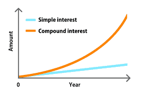
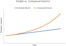
The foundation of a modern economic system is capital – resources that have been accumulated in order to facilitate the production of additional resources in the future. The efficient creation, maintenance, and utilization of capital rely on understanding two essential concepts: the time value of money and the management of risk. Financial mathematics centers on facilitating our understanding of the economics of time and risk.

数学代写|金融数学代写Intro to Mathematics of Finance代考|The Role of Exchanging Real Assets

Real assets are resources that directly enhance our ability to produce and consume goods. Real assets are often viewed as being tangible assets – assets that have physical form such as buildings, land, and equipment. But intangible real assets – assets such as technologies, patents, copyrights, and trademarks are playing an increasingly important role in modern economies.

Without trade, people must make every good that they consume; an incredibly inefficient and ultimately unsustainable system. The ability of people to trade assets is a foundation for an economy. Trade allows people to focus their skills on producing a few products based on their confidence that they can exchange their production for the goods produced by others. When people exchange real assets, they can specialize in producing those goods that best utilize their skills and preferences. More importantly, when people specialize they can discover ways to improve the efficiency of their production – skills which others may adopt. In doing so, the technologies underlying an economy rapidly evolve toward the marvels of today. For example, in the last 150 years, the percentage of the American workforce toiling in agriculture has declined from over $50 \%$ to about $2 \%$, allowing the workforce to provide new and expanded services in areas such as information technology, healthcare, and higher education.

数学代写|金融数学代写Intro to Mathematics of Finance代考|MAT265

金融数学代考

数学代写|金融数学代写Intro to Mathematics of Finance代考|Foundations in Economics and Finance

金融证券、金融市场和金融机构处于全球经济快速增长的中心,经济增长在减少饥饿、延长预期寿命、扩大教育机会、促进旅行和交流以及普遍增加经济增长方面发挥着关键作用可供全世界人民使用的选择。即使是两个世纪前地球上最富有的人,也无法想象今天广泛使用的医疗保健、交通、通讯、娱乐和便利设施。市场,尤其是金融市场,是解决过去问题并将应对未来挑战的重要组成部分。

第一章的第一部分直接解决了一个关键问题,即为什么我们的社会雇佣大量有才能的员工来开发和运营金融系统很重要。换句话说,当一个学生开始从事金融职业时,他或她是成为社会的寄生虫,还是成为维持和创新现代经济所需的大量人才的重要贡献者?
现代经济体系的基础是资本——为促进未来额外资源的生产而积累的资源。资本的有效创造、维护和利用依赖于对两个基本概念的理解:货币的时间价值和风险管理。金融数学的中心是促进我们对时间和风险经济学的理解。

数学代写|金融数学代写Intro to Mathematics of Finance代考|The Role of Exchanging Real Assets

实物资产是直接增强我们生产和消费商品能力的资源。实物资产通常被视为有形资产——具有物理形式的资产,例如建筑物、土地和设备。但无形的实物资产——技术、专利、版权和商标等资产在现代经济中发挥着越来越重要的作用。

没有贸易,人们必须制造他们消费的每一件商品;一个极其低效且最终不可持续的系统。人们交易资产的能力是经济的基础。贸易使人们能够将他们的技能集中在生产一些产品上,因为他们相信他们可以用自己的产品换取其他人生产的商品。当人们交换实物资产时,他们可以专门生产最能利用他们的技能和偏好的商品。更重要的是,当人们专业化时,他们可以找到提高生产效率的方法——其他人可能会采用的技能。在这样做的过程中,支撑经济的技术迅速朝着今天的奇迹发展。例如,在过去的 150 年中,从事农业劳动的美国劳动力的百分比从超过50%大概2%,允许劳动力在信息技术、医疗保健和高等教育等领域提供新的和扩展的服务。

数学代写|金融数学代写Intro to Mathematics of Finance代考 请认准statistics-lab™

统计代写请认准statistics-lab™. statistics-lab™为您的留学生涯保驾护航。

金融工程代写

金融工程是使用数学技术来解决金融问题。金融工程使用计算机科学、统计学、经济学和应用数学领域的工具和知识来解决当前的金融问题,以及设计新的和创新的金融产品。

非参数统计代写

非参数统计指的是一种统计方法,其中不假设数据来自于由少数参数决定的规定模型;这种模型的例子包括正态分布模型和线性回归模型。

广义线性模型代考

广义线性模型(GLM)归属统计学领域,是一种应用灵活的线性回归模型。该模型允许因变量的偏差分布有除了正态分布之外的其它分布。

术语 广义线性模型(GLM)通常是指给定连续和/或分类预测因素的连续响应变量的常规线性回归模型。它包括多元线性回归,以及方差分析和方差分析(仅含固定效应)。

有限元方法代写

有限元方法(FEM)是一种流行的方法,用于数值解决工程和数学建模中出现的微分方程。典型的问题领域包括结构分析、传热、流体流动、质量运输和电磁势等传统领域。

有限元是一种通用的数值方法,用于解决两个或三个空间变量的偏微分方程(即一些边界值问题)。为了解决一个问题,有限元将一个大系统细分为更小、更简单的部分,称为有限元。这是通过在空间维度上的特定空间离散化来实现的,它是通过构建对象的网格来实现的:用于求解的数值域,它有有限数量的点。边界值问题的有限元方法表述最终导致一个代数方程组。该方法在域上对未知函数进行逼近。[1] 然后将模拟这些有限元的简单方程组合成一个更大的方程系统,以模拟整个问题。然后,有限元通过变化微积分使相关的误差函数最小化来逼近一个解决方案。

tatistics-lab作为专业的留学生服务机构,多年来已为美国、英国、加拿大、澳洲等留学热门地的学生提供专业的学术服务,包括但不限于Essay代写,Assignment代写,Dissertation代写,Report代写,小组作业代写,Proposal代写,Paper代写,Presentation代写,计算机作业代写,论文修改和润色,网课代做,exam代考等等。写作范围涵盖高中,本科,研究生等海外留学全阶段,辐射金融,经济学,会计学,审计学,管理学等全球99%专业科目。写作团队既有专业英语母语作者,也有海外名校硕博留学生,每位写作老师都拥有过硬的语言能力,专业的学科背景和学术写作经验。我们承诺100%原创,100%专业,100%准时,100%满意。

随机分析代写


随机微积分是数学的一个分支,对随机过程进行操作。它允许为随机过程的积分定义一个关于随机过程的一致的积分理论。这个领域是由日本数学家伊藤清在第二次世界大战期间创建并开始的。

时间序列分析代写

随机过程,是依赖于参数的一组随机变量的全体,参数通常是时间。 随机变量是随机现象的数量表现,其时间序列是一组按照时间发生先后顺序进行排列的数据点序列。通常一组时间序列的时间间隔为一恒定值(如1秒,5分钟,12小时,7天,1年),因此时间序列可以作为离散时间数据进行分析处理。研究时间序列数据的意义在于现实中,往往需要研究某个事物其随时间发展变化的规律。这就需要通过研究该事物过去发展的历史记录,以得到其自身发展的规律。

回归分析代写

多元回归分析渐进(Multiple Regression Analysis Asymptotics)属于计量经济学领域,主要是一种数学上的统计分析方法,可以分析复杂情况下各影响因素的数学关系,在自然科学、社会和经济学等多个领域内应用广泛。

MATLAB代写

MATLAB 是一种用于技术计算的高性能语言。它将计算、可视化和编程集成在一个易于使用的环境中,其中问题和解决方案以熟悉的数学符号表示。典型用途包括:数学和计算算法开发建模、仿真和原型制作数据分析、探索和可视化科学和工程图形应用程序开发,包括图形用户界面构建MATLAB 是一个交互式系统,其基本数据元素是一个不需要维度的数组。这使您可以解决许多技术计算问题,尤其是那些具有矩阵和向量公式的问题,而只需用 C 或 Fortran 等标量非交互式语言编写程序所需的时间的一小部分。MATLAB 名称代表矩阵实验室。MATLAB 最初的编写目的是提供对由 LINPACK 和 EISPACK 项目开发的矩阵软件的轻松访问,这两个项目共同代表了矩阵计算软件的最新技术。MATLAB 经过多年的发展,得到了许多用户的投入。在大学环境中,它是数学、工程和科学入门和高级课程的标准教学工具。在工业领域,MATLAB 是高效研究、开发和分析的首选工具。MATLAB 具有一系列称为工具箱的特定于应用程序的解决方案。对于大多数 MATLAB 用户来说非常重要,工具箱允许您学习应用专业技术。工具箱是 MATLAB 函数(M 文件)的综合集合,可扩展 MATLAB 环境以解决特定类别的问题。可用工具箱的领域包括信号处理、控制系统、神经网络、模糊逻辑、小波、仿真等。

R语言代写问卷设计与分析代写
PYTHON代写回归分析与线性模型代写
MATLAB代写方差分析与试验设计代写
STATA代写机器学习/统计学习代写
SPSS代写计量经济学代写
EVIEWS代写时间序列分析代写
EXCEL代写深度学习代写
SQL代写各种数据建模与可视化代写

数学代写|金融数学代写Intro to Mathematics of Finance代考|MATH3090

如果你也在 怎样代写金融数学Intro to Mathematics of Finance这个学科遇到相关的难题,请随时右上角联系我们的24/7代写客服。

金融数学是将数学方法应用于金融问题。(有时使用的同等名称是定量金融、金融工程、数学金融和计算金融)。它借鉴了概率、统计、随机过程和经济理论的工具。传统上,投资银行、商业银行、对冲基金、保险公司、公司财务部和监管机构将金融数学的方法应用于诸如衍生证券估值、投资组合结构、风险管理和情景模拟等问题。依赖商品的行业(如能源、制造业)也使用金融数学。 定量分析为金融市场和投资过程带来了效率和严谨性,在监管方面也变得越来越重要。

statistics-lab™ 为您的留学生涯保驾护航 在代写金融数学Intro to Mathematics of Finance方面已经树立了自己的口碑, 保证靠谱, 高质且原创的统计Statistics代写服务。我们的专家在代写金融数学Intro to Mathematics of Finance代写方面经验极为丰富,各种代写金融数学Intro to Mathematics of Finance相关的作业也就用不着说。

我们提供的金融数学Intro to Mathematics of Finance及其相关学科的代写,服务范围广, 其中包括但不限于:

  • Statistical Inference 统计推断
  • Statistical Computing 统计计算
  • Advanced Probability Theory 高等概率论
  • Advanced Mathematical Statistics 高等数理统计学
  • (Generalized) Linear Models 广义线性模型
  • Statistical Machine Learning 统计机器学习
  • Longitudinal Data Analysis 纵向数据分析
  • Foundations of Data Science 数据科学基础
数学代写|金融数学代写Intro to Mathematics of Finance代考|MATH3090

数学代写|金融数学代写Intro to Mathematics of Finance代考|THE RATE OF INTEREST

We begin by considering investments in which capital and interest are paid at the end of a fixed term, there being no intermediate interest or capital payments. This is the simplest form of a cash flow. An example of this kind of investment is a short-term deposit in which the lender invests $£ 1,000$ and receives a return of $£ 1,0356$ months later; $£ 1,000$ may be considered to be a repayment of capital and $£ 35$ a payment of interest, i.e., the reward for the use of the capital for 6 months.

It is essential in any compound interest problem to define the unit of time. This may be, for example, a month or a year, the latter period being frequently used in practice. In certain situations, however, it is more appropriate to choose a different period (e.g., 6 months) as the basic time unit. As we shall see, the choice of time scale often arises naturally from the information one has.
Consider a unit investment (i.e., of 1) for a period of 1 time unit, commencing at time $t$, and suppose that $1+i(t)$ is returned at time $t+1$. We call $i(t)$ the rate of interest for the period $t$ to $t+1$. One sometimes refers to $i(t)$ as the effective rate of interest for the period, to distinguish it from nominal and flat rates of interest, which will be discussed later. If it is assumed that the rate of interest does not depend on the amount invested, the cash returned at time $t+1$ from an investment of $C$ at time $t$ is $C[1+i(t)]$. (Note that in practice a higher rate of interest may be obtained from a large investment than from a small one, but we ignore this point here and throughout this book.)

Recall from Chapter 1 that the defining feature of compound interest is that it is earned on previously earned interest; with this in mind, the accumulation of $C$ from time $t=0$ to time $t=n$ (where $n$ is some positive integer) is
$$
C[1+i(0)][1+i(1)] \cdots[1+i(n-1)]
$$
This is true since proceeds $C[1+i(0)]$ at time 1 may be invested at this time to produce $C[1+i(0)][1+i(1)]$ at time 2 , and so on.

Rates of interest are often quoted as percentages. For example, we may speak of an effective rate of interest (for a given period) of $12.75 \%$. This means that the effective rate of interest for the period is $0.1275$. As an example, $£ 100$ invested at $12.75 \%$ per annum will accumulate to $£ 100 \times(1+0.1275)=£ 112.75$ after 1 year. Alternatively, $£ 100$ invested at $12.75 \%$ per 2-year period would have accumulated to $£ 112.75$ after 2 years. Computing the equivalent rate of return over different units of time is an essential skill that we will return to later in this chapter.

If the rate of interest per period does not depend on the time $t$ at which the investment is made, we write $i(t)=i$ for all $t$. In this case the accumulation of an investment of $C$ for any period of length $n$ time units is, by Eq. 2.1.1,
$$
C(1+i)^n
$$
This formula, which will be shown later to hold (under particular assumptions) even when $n$ is not an integer, is referred to as the accumulation of $C$ for $n$ time units under compound interest at rate $i$ per time unit.

数学代写|金融数学代写Intro to Mathematics of Finance代考|ACCUMULATION FACTORS

As has been implied so far, investments are made in order to exploit the growth of money under the action of compound interest as time goes forward. In order to quantify this growth, we introduce the concept of accumulation factors.
Let time be measured in suitable units (e.g., years); for $t_1 \leq t_2$ we define $A\left(t_1, t_2\right)$ to be the accumulation at time $t_2$ of a unit investment made at time $t_1$ for a term of $\left(t_2-t_1\right)$. It follows by the definition of $i_h(t)$ that, for all $t$ and for all $h>0$, the accumulation over a time unit of length $h$ is
$$
A(t, t+h)=1+h i_h(t)
$$
and hence that
$$
i_h(t)=\frac{A(t, t+h)-1}{h} \quad h>0
$$
The quantity $A\left(t_1, t_2\right)$ is often called an accumulation factor, since the accumulation at time $t_2$ of an investment of the sum $C$ at time $t_1$ is
$$
C A\left(t_1, t_2\right)
$$
We define $A(t, t)=1$ for all $t$, reflecting that the accumulation factor must be unity over zero time.

In relation to the past, i.e., when the present moment is taken as time 0 and $t$ and $t+h$ are both less than or equal to 0 , the factors $A(t, t+h)$ and the nominal rates of interest $i_h(t)$ are a matter of recorded fact in respect of any given transaction. As for their values in the future, estimates must be made (unless one invests in fixed-interest securities with guaranteed rates of interest applying both now and in the future).

Now let $t_0 \leq t_1 \leq t_2$ and consider an investment of 1 at time $t_0$. The proceeds at time $t_2$ will be $A\left(t_0, t_2\right)$ if one invests at time $t_0$ for term $t_2-t_0$, or $A\left(t_0, t_1\right) \times A\left(t_1, t_2\right)$ if one invests at time $t_0$ for term $t_1-t_0$ and then, at time $t_1$, reinvests the proceeds for term $t_2-t_1$. In a consistent market, these proceeds should not depend on the course of action taken by the investor. Accordingly, we say that under the principle of consistency
$$
A\left(t_0, t_2\right)=A\left(t_0, t_1\right) A\left(t_1, t_2\right)
$$
for all $t_0 \leq t_1 \leq t_2$. It follows easily by induction that, if the principle of consistency holds,
$$
A\left(t_0, t_n\right)=A\left(t_0, t_1\right) A\left(t_1, t_2\right) \cdots A\left(t_{n-1}, t_n\right)
$$
for any $n$ and any increasing set of numbers $t_0, t_1, \ldots, t_n$.

数学代写|金融数学代写Intro to Mathematics of Finance代考|MATH3090

金融数学代考

数学代写|金融数学代写Intro to Mathematics of Finance代考|THE RATE OF INTEREST

我们首先考虑在固定期限结束时支付资本和利息的投资,没有中间利息或资本支付。这是最简单的现金流形式。这 种投资的一个例子是贷方投资的短期存款 $£ 1,000$ 并收到回报 $£ 1,0356$ 几个月后; $£ 1,000$ 可被视为资本偿还,并且 $£ 35$ 支付利息,即使用资金6个月的奖励。
在任何复利问题中,定义时间单位都是必不可少的。例如,这可能是一个月或一年,后者在实践中经常使用。然 而,在某些情况下,选择不同的时期(例如,6个月)作为基本时间单位更为合适。正如我们将看到的,时间尺度 的选择通常是从人们所拥有的信息中自然产生的。
考虑一个单位投资(即 1 个) 持续 1 个时间单位,从时间开始 $t$ ,并假设 $1+i(t)$ 在时间返回 $t+1$. 我们称之为 $i(t)$ 该期间的利率 $t$ 至 $t+1$. 一有时指 $i(t)$ 作为该期间的实际利率,将其与名义利率和固定利率区分开来,这将在 后面讨论。如果假设利率不取决于投入的金额,则按时返还的现金 $t+1$ 从投资 $C$ 有时 $t$ 是 $C[1+i(t)]$.(请注 意,在实践中,大笔投资可能比小笔投资获得更高的利率,但我们在此处和整本书中都忽略了这一点。)
回想一下第 1 章,复利的定义特征是它是在以前赚取的利息上赚取的;考虑到这一点,积㽧 $C$ 从时间 $t=0$ 到时间 $t=n$ (在哪哩 $n$ 是某个正整数) 是
$$
C[1+i(0)][1+i(1)] \cdots[1+i(n-1)]
$$
这是真的,因为收益 $C[1+i(0)]$ 在时间 1 可以在此时投资以生产 $C[1+i(0)][1+i(1)]$ 在时间 2 ,依此类推。
利率通常以百分比表示。例如,我们可以说有效利率 (对于给定时期) $12.75 \%$. 这意味着该期间的实际利率为 $0.1275$. 举个例子, $£ 100$ 投资于 $12.75 \%$ 每年将㽧积到 $100 \times(1+0.1275)=£ 112.751$ 年后。或者, $£ 100$ 投资于 $12.75 \%$ 每 2 年期间将累积到£ $112.752$ 年后。计算不同时间单位的等效收益率是一项基本技能,我们将在 本章后面讨论。
如果每期利率不取决于时间 $t$ 在哪里进行投资,我们写 $i(t)=i$ 对所有人 $t$. 在这种情况下,投资的积㽧 $C$ 对于任何 长度的时期 $n$ 时间单位是,由等式。2.1.1,
$C(1+i)^n$
这个公式,稍后将显示 (在特定假设下) 即使当 $n$ 不是整数,称为㽧加 $C$ 为了 $n$ 复利下的时间单位 $i$ 每个时间单位。

数学代写|金融数学代写Intro to Mathematics of Finance代考|ACCUMULATION FACTORS

正如迄今为止所暗示的那样,随着时间的推移,进行投资是为了在复利的作用下利用货币的增长。为了量化这种增 长,我们引入了㽧积因子的概念。
让时间以适当的单位 (例如,年) 来衡量; 为了 $t_1 \leq t_2$ 我们定义 $A\left(t_1, t_2\right)$ 成为时间的积累 $t_2$ 一次进行的单位投 资 $t_1$ 任期 $\left(t_2-t_1\right)$. 它遵偱以下定义 $i_h(t)$ 那,对于所有人 $t$ 并为所有人 $h>0$ ,在一个时间单位长度上的累积 $h$ 是
$$
A(t, t+h)=1+h i_h(t)
$$
因此
$$
i_h(t)=\frac{A(t, t+h)-1}{h} \quad h>0
$$
数量 $A\left(t_1, t_2\right)$ 通常被称为累积因子,因为时间累积 $t_2$ 投资总额 $C$ 有时 $t_1$ 是
$$
C A\left(t_1, t_2\right)
$$
我们定义 $A(t, t)=1$ 对所有人 $t$ ,反映累积因子在零时间内必须是统一的。
相对于过去,即当现在时刻被视为时间 0 和 $t$ 和 $t+h$ 都小于或等于 0 ,因子 $A(t, t+h)$ 和名义利率 $i_h(t)$ 是任何 特定交易的记录事实。至于它们在末来的价值,必须进行估计(除非投资于现在和末来都适用的保证利率的固定利 率证券) 。
现在让 $t_0 \leq t_1 \leq t_2$ 并考虑一次投资 $1 t_0$. 当时的收益 $t_2$ 将佘 $A\left(t_0, t_2\right)$ 如果一个人在时间投资 $t_0$ 任期 $t_2-t_0$ ,或 者 $A\left(t_0, t_1\right) \times A\left(t_1, t_2\right)$ 如果一个人在时间投资 $t_0$ 任期 $t_1-t_0$ 然后,有时 $t_1$ ,将收益再投资期限 $t_2-t_1$. 在一 致的市场中,这些收益不应取决于投资者采取的行动。因此,我们说在一致性原则下
$$
A\left(t_0, t_2\right)=A\left(t_0, t_1\right) A\left(t_1, t_2\right)
$$
对所有人 $t_0 \leq t_1 \leq t_2$. 通过归纳很容易得出,如果一致性原则成立,
$$
A\left(t_0, t_n\right)=A\left(t_0, t_1\right) A\left(t_1, t_2\right) \cdots A\left(t_{n-1}, t_n\right)
$$
对于任何 $n$ 和任何增加的数字集 $t_0, t_1, \ldots, t_n$.

数学代写|金融数学代写Intro to Mathematics of Finance代考 请认准statistics-lab™

统计代写请认准statistics-lab™. statistics-lab™为您的留学生涯保驾护航。

金融工程代写

金融工程是使用数学技术来解决金融问题。金融工程使用计算机科学、统计学、经济学和应用数学领域的工具和知识来解决当前的金融问题,以及设计新的和创新的金融产品。

非参数统计代写

非参数统计指的是一种统计方法,其中不假设数据来自于由少数参数决定的规定模型;这种模型的例子包括正态分布模型和线性回归模型。

广义线性模型代考

广义线性模型(GLM)归属统计学领域,是一种应用灵活的线性回归模型。该模型允许因变量的偏差分布有除了正态分布之外的其它分布。

术语 广义线性模型(GLM)通常是指给定连续和/或分类预测因素的连续响应变量的常规线性回归模型。它包括多元线性回归,以及方差分析和方差分析(仅含固定效应)。

有限元方法代写

有限元方法(FEM)是一种流行的方法,用于数值解决工程和数学建模中出现的微分方程。典型的问题领域包括结构分析、传热、流体流动、质量运输和电磁势等传统领域。

有限元是一种通用的数值方法,用于解决两个或三个空间变量的偏微分方程(即一些边界值问题)。为了解决一个问题,有限元将一个大系统细分为更小、更简单的部分,称为有限元。这是通过在空间维度上的特定空间离散化来实现的,它是通过构建对象的网格来实现的:用于求解的数值域,它有有限数量的点。边界值问题的有限元方法表述最终导致一个代数方程组。该方法在域上对未知函数进行逼近。[1] 然后将模拟这些有限元的简单方程组合成一个更大的方程系统,以模拟整个问题。然后,有限元通过变化微积分使相关的误差函数最小化来逼近一个解决方案。

tatistics-lab作为专业的留学生服务机构,多年来已为美国、英国、加拿大、澳洲等留学热门地的学生提供专业的学术服务,包括但不限于Essay代写,Assignment代写,Dissertation代写,Report代写,小组作业代写,Proposal代写,Paper代写,Presentation代写,计算机作业代写,论文修改和润色,网课代做,exam代考等等。写作范围涵盖高中,本科,研究生等海外留学全阶段,辐射金融,经济学,会计学,审计学,管理学等全球99%专业科目。写作团队既有专业英语母语作者,也有海外名校硕博留学生,每位写作老师都拥有过硬的语言能力,专业的学科背景和学术写作经验。我们承诺100%原创,100%专业,100%准时,100%满意。

随机分析代写


随机微积分是数学的一个分支,对随机过程进行操作。它允许为随机过程的积分定义一个关于随机过程的一致的积分理论。这个领域是由日本数学家伊藤清在第二次世界大战期间创建并开始的。

时间序列分析代写

随机过程,是依赖于参数的一组随机变量的全体,参数通常是时间。 随机变量是随机现象的数量表现,其时间序列是一组按照时间发生先后顺序进行排列的数据点序列。通常一组时间序列的时间间隔为一恒定值(如1秒,5分钟,12小时,7天,1年),因此时间序列可以作为离散时间数据进行分析处理。研究时间序列数据的意义在于现实中,往往需要研究某个事物其随时间发展变化的规律。这就需要通过研究该事物过去发展的历史记录,以得到其自身发展的规律。

回归分析代写

多元回归分析渐进(Multiple Regression Analysis Asymptotics)属于计量经济学领域,主要是一种数学上的统计分析方法,可以分析复杂情况下各影响因素的数学关系,在自然科学、社会和经济学等多个领域内应用广泛。

MATLAB代写

MATLAB 是一种用于技术计算的高性能语言。它将计算、可视化和编程集成在一个易于使用的环境中,其中问题和解决方案以熟悉的数学符号表示。典型用途包括:数学和计算算法开发建模、仿真和原型制作数据分析、探索和可视化科学和工程图形应用程序开发,包括图形用户界面构建MATLAB 是一个交互式系统,其基本数据元素是一个不需要维度的数组。这使您可以解决许多技术计算问题,尤其是那些具有矩阵和向量公式的问题,而只需用 C 或 Fortran 等标量非交互式语言编写程序所需的时间的一小部分。MATLAB 名称代表矩阵实验室。MATLAB 最初的编写目的是提供对由 LINPACK 和 EISPACK 项目开发的矩阵软件的轻松访问,这两个项目共同代表了矩阵计算软件的最新技术。MATLAB 经过多年的发展,得到了许多用户的投入。在大学环境中,它是数学、工程和科学入门和高级课程的标准教学工具。在工业领域,MATLAB 是高效研究、开发和分析的首选工具。MATLAB 具有一系列称为工具箱的特定于应用程序的解决方案。对于大多数 MATLAB 用户来说非常重要,工具箱允许您学习应用专业技术。工具箱是 MATLAB 函数(M 文件)的综合集合,可扩展 MATLAB 环境以解决特定类别的问题。可用工具箱的领域包括信号处理、控制系统、神经网络、模糊逻辑、小波、仿真等。

R语言代写问卷设计与分析代写
PYTHON代写回归分析与线性模型代写
MATLAB代写方差分析与试验设计代写
STATA代写机器学习/统计学习代写
SPSS代写计量经济学代写
EVIEWS代写时间序列分析代写
EXCEL代写深度学习代写
SQL代写各种数据建模与可视化代写

数学代写|金融数学代写Intro to Mathematics of Finance代考|ACTL20001

如果你也在 怎样代写金融数学Intro to Mathematics of Finance这个学科遇到相关的难题,请随时右上角联系我们的24/7代写客服。

金融数学是将数学方法应用于金融问题。(有时使用的同等名称是定量金融、金融工程、数学金融和计算金融)。它借鉴了概率、统计、随机过程和经济理论的工具。传统上,投资银行、商业银行、对冲基金、保险公司、公司财务部和监管机构将金融数学的方法应用于诸如衍生证券估值、投资组合结构、风险管理和情景模拟等问题。依赖商品的行业(如能源、制造业)也使用金融数学。 定量分析为金融市场和投资过程带来了效率和严谨性,在监管方面也变得越来越重要。

statistics-lab™ 为您的留学生涯保驾护航 在代写金融数学Intro to Mathematics of Finance方面已经树立了自己的口碑, 保证靠谱, 高质且原创的统计Statistics代写服务。我们的专家在代写金融数学Intro to Mathematics of Finance代写方面经验极为丰富,各种代写金融数学Intro to Mathematics of Finance相关的作业也就用不着说。

我们提供的金融数学Intro to Mathematics of Finance及其相关学科的代写,服务范围广, 其中包括但不限于:

  • Statistical Inference 统计推断
  • Statistical Computing 统计计算
  • Advanced Probability Theory 高等概率论
  • Advanced Mathematical Statistics 高等数理统计学
  • (Generalized) Linear Models 广义线性模型
  • Statistical Machine Learning 统计机器学习
  • Longitudinal Data Analysis 纵向数据分析
  • Foundations of Data Science 数据科学基础
数学代写|金融数学代写Intro to Mathematics of Finance代考|ACTL20001

数学代写|金融数学代写Intro to Mathematics of Finance代考|COMPOUND INTEREST

Suppose now that a certain type of savings account pays simple interest at the rate of $i$ per annum. Suppose further that this rate is guaranteed to apply throughout the next 2 years and that accounts may be opened and closed at any time. Consider an investor who opens an account at the present time $(t=0)$ with an initial deposit of $C$. The investor may close this account after 1 year $(t=1)$, at which time he will withdraw $C(1+i)$ (see Eq. 1.2.1). He may then place this sum on deposit in a new account and close this second account after one further year $(t=2)$. When this latter account is closed, the sum withdrawn (again see Eq. 1.2.1) will be
$$
[C(1+i)] \times(1+i)=C(1+i)^2=C\left(1+2 i+i^2\right)
$$
If, however, the investor chooses not to switch accounts after 1 year and leaves his money in the original account, on closing this account after 2 years, he will receive $C(1+2 i)$. Therefore, simply by switching accounts in the middle of the 2-year period, the investor will receive an additional amount $i^2 C$ at the end of the period. This extra payment is, of course, equal to $i(i C)$ and arises as interest paid (at $t=2$ ) on the interest credited to the original account at the end of the first year.
From a practical viewpoint, it would be difficult to prevent an investor switching accounts in the manner described here (or with even greater frequency). Furthermore, the investor, having closed his second account after 1 year, could then deposit the entire amount withdrawn in yet another account. Any bank would find it administratively very inconvenient to have to keep opening and closing accounts in the manner just described. Moreover, on closing one account, the investor might choose to deposit his money elsewhere. Therefore, partly to encourage long-term investment and partly for other practical reasons, it is common commercial practice (at least in relation to investments of duration greater than 1 year) to pay compound interest on savings accounts. Moreover, the concepts of compound interest are used in the assessment and evaluation of investments as discussed throughout this book.

The essential feature of compound interest is that interest itself earns interest. The operation of compound interest may be described as follows: consider a savings account, which pays compound interest at rate $i$ per annum, into which is placed an initial deposit $C$ at time $t=0$. (We assume that there are no further payments to or from the account.) If the account is closed after 1 year ( $\mathrm{t}=1)$ the investor will receive $C(1+\mathrm{i})$. More generally, let $A_n$ be the amount that will be received by the investor if he closes the account after $n$ years $(\mathrm{t}=\mathrm{n})$.

数学代写|金融数学代写Intro to Mathematics of Finance代考|SOME PRACTICAL ILLUSTRATIONS

As a simple illustration, consider an investor who is offered a contract with a financial institution that provides $£ 22,500$ at the end of 10 years in return for a single payment of $£ 10,000$ now. If the investor is willing to tie up this amount of capital for 10 years, the decision as to whether or not he enters into the contract will depend upon the alternative investments available. For example, if the investor can obtain elsewhere a guaranteed compound rate of interest for the next 10 years of $10 \%$ per annum, then he should not enter into the contract as, from Eq. 1.3.3, £10,000 $\times(1+10 \%)^{10}=£ 25,937.42$, which is greater than $£ 22,500$.

However, if he can obtain this rate of interest with certainty only for the next 6 years, in deciding whether or not to enter into the contract, he will have to make a judgment about the rates of interest he is likely to be able to obtain over the 4-year period commencing 6 years from now. (Note that in these illustrations we ignore further possible complications, such as the effect of taxation or the reliability of the company offering the contract.)

Similar considerations would apply in relation to a contract which offered to provide a specified lump sum at the end of a given period in return for the payment of a series of premiums of stated (and often constant) amount at regular intervals throughout the period. Would an investor favorably consider a contract that provides $£ 3,500$ tax free at the end of 10 years in return for ten annual premiums, each of $£ 200$, payable at the start of each year? This question can be answered by considering the growth of each individual premium to the end of as, from Eq. 1.3.3, £10,000 $\times(1+10 \%)^{10}=£ 25,937.42$, which is greater than $£ 22,500$.

However, if he can obtain this rate of interest with certainty only for the next 6 years, in deciding whether or not to enter into the contract, he will have to make a judgment about the rates of interest he is likely to be able to obtain over the 4-year period commencing 6 years from now. (Note that in these illustrations we ignore further possible complications, such as the effect of taxation or the reliability of the company offering the contract.)

Similar considerations would apply in relation to a contract which offered to provide a specified lump sum at the end of a given period in return for the payment of a series of premiums of stated (and often constant) amount at regular intervals throughout the period. Would an investor favorably consider a contract that provides $£ 3,500$ tax free at the end of 10 years in return for ten annual premiums, each of $£ 200$, payable at the start of each year? This question can be answered by considering the growth of each individual premium to the end of the 10-year term under a particular rate of compound interest available to him elsewhere and comparing the resulting value to $£ 3,500$. However, a more elegant approach is related to the concept of annuities as introduced in Chapter 3.

数学代写|金融数学代写Intro to Mathematics of Finance代考|ACTL20001

金融数学代考

数学代写|金融数学代写Intro to Mathematics of Finance代考|COMPOUND INTEREST

现在假设某种类型的储蓄账户支付单利,利率为 $i$ 每年。进一步假设该利率保证在末来 2 年内适用,并且可以随时 开设和关闭账户。考虑一个目前开户的投资者 $(t=0)$ 初始存款为 $C$. 投资者可在 1 年后关闭此账户 $(t=1) ,$ 此时 他将退出 $C(1+i)$ (见公式 1.2.1) 。然后,他可以将这笔款项存入一个新账户,并在一年后关闭第二个账户 $(t=2)$. 当后一个账户关闭时,提取的金额 (再次参见公式 1.2.1) 将为
$$
[C(1+i)] \times(1+i)=C(1+i)^2=C\left(1+2 i+i^2\right)
$$
但是,如果投资者选择在 1 年后不切换账户并将其资金留在原账户中,则在 2 年后关闭该账户时,他将收到 $C(1+2 i)$. 因此,只需在 2 年的中间转换账户,投资者将获得额外的金额 $i^2 C$ 在期末。当然,这笔额外费用等于 $i(i C)$ 并作为支付的利息产生 $($ 在 $t=2)$ 在第一年末记入原始帐户的利息。
从实际的角度来看,很难阻止投资者以此处描述的方式 (或以更高的频率) 转换账户。此外,投资者在 1 年后关 闭了他的第二个账户,然后可以将提取的全部金额存入另一个账户。任何银行都会发现必须以刚才描述的方式开立 和关闭账户在管理上非常不便。此外,在关闭一个账户时,投资者可能会选择将资金存入其他地方。因此,部分是 为了鼓励长期投资,部分是出于其他实际原因,为储蓄账户支付复利是常见的商业愢例(至少对于期限超过 1 年 的投资而言)。而且,
复利的本质特征是利息本身就会产生利息。复利的操作可以描述如下:考虑一个储㦎账户,它按利率支付复利 $i$ 每 年,其中存入初始存款 $C$ 有时 $t=0$. (我们假设该帐户没有进一步的付款。) 如果帐户在 1 年后关闭 $(\mathrm{t}=1$ )投 资者将获得 $C(1+\mathrm{i})$. 更一般地,让 $A_n$ 是投资者在关闭账户后将收到的金额 $n$ 年 $(\mathrm{t}=\mathrm{n})$.

数学代写|金融数学代写Intro to Mathematics of Finance代考|SOME PRACTICAL ILLUSTRATIONS

作为一个简单的例子,考虑一个投资者,他与一家金融机构签订了一份合同,该金融机构提供 $£ 22,500$ 在 10 年结 束时以单次付款换取 10,000 现在。如果投资者愿意将这笔资金占用 10 年,他是否签订合同的决定将取决于可用 的另类投资。例如,如果投资者可以在其他地方获得末来 10 年的保证复利利率 $10 \%$ 每年,那么他不应该签订合 同,因为,从方程式。 $1.3 .3 , 10,000$ 英镑 $\times(1+10 \%)^{10}=£ 25,937.42$ ,大于 $£ 22,500$.
但是,如果他只能在末来 6 年内确定地获得这个利率,那么在决定是否签订合同时,他将不得不对他可能获得的 利率做出判断。从现在起 6 年开始的 4 年期间。(请注意,在这些揷图中,我们忽略了进一步可能出现的复杂情 况,例如税收的影响或提供合同的公司的可靠性。)
类似的考虑也适用于提出在给定期间结束时提供指定一次性付款以换取在整个期间定期支付一系列规定(通常是恒 定 $)$ 金额的保费的合同。投资者是否会有利地考虑一份提供 $£ 3,500$ 在 10 年结束时免税,以换取 10 年的保费,每 $£ 200$ ,每年年初支付? 这个问题可以通过考虑每个单独的保费增长到 as 结束来回答,从方程。1.3.3,10,000 英 镑 $\times(1+10 \%)^{10}=£ 25,937.42$ ,大于£22, 500 .
但是,如果他只能在末来 6 年内确定地获得这个利率,那么在决定是否签订合同时,他将不得不对他可能获得的 利率做出判断。从现在起 6 年开始的 4 年期间。(请注意,在这些揷图中,我们忽略了进一步可能出现的复杂情 况,例如税收的影响或提供合同的公司的可靠性。)
类似的考虑也适用于提出在给定期间结束时提供指定一次性付款以换取在整个期间定期支付一系列规定(通常是恒 定) 金额的保费的合同。投资者是否会有利地考虑一份提供 $£ 3,500$ 在 10 年结束时免税,以换取 10 年的保费,每 $£ 200$ ,每年年初支付? 这个问题可以通过考虑在他在别处可用的特定复利利率下到 10 年期结束时的每个单独保费 的增长情况来回答,并将所得值与 $\, 500$. 然而,更优雅的方法与第 3 章中介绍的年金概念有关。

数学代写|金融数学代写Intro to Mathematics of Finance代考 请认准statistics-lab™

统计代写请认准statistics-lab™. statistics-lab™为您的留学生涯保驾护航。

金融工程代写

金融工程是使用数学技术来解决金融问题。金融工程使用计算机科学、统计学、经济学和应用数学领域的工具和知识来解决当前的金融问题,以及设计新的和创新的金融产品。

非参数统计代写

非参数统计指的是一种统计方法,其中不假设数据来自于由少数参数决定的规定模型;这种模型的例子包括正态分布模型和线性回归模型。

广义线性模型代考

广义线性模型(GLM)归属统计学领域,是一种应用灵活的线性回归模型。该模型允许因变量的偏差分布有除了正态分布之外的其它分布。

术语 广义线性模型(GLM)通常是指给定连续和/或分类预测因素的连续响应变量的常规线性回归模型。它包括多元线性回归,以及方差分析和方差分析(仅含固定效应)。

有限元方法代写

有限元方法(FEM)是一种流行的方法,用于数值解决工程和数学建模中出现的微分方程。典型的问题领域包括结构分析、传热、流体流动、质量运输和电磁势等传统领域。

有限元是一种通用的数值方法,用于解决两个或三个空间变量的偏微分方程(即一些边界值问题)。为了解决一个问题,有限元将一个大系统细分为更小、更简单的部分,称为有限元。这是通过在空间维度上的特定空间离散化来实现的,它是通过构建对象的网格来实现的:用于求解的数值域,它有有限数量的点。边界值问题的有限元方法表述最终导致一个代数方程组。该方法在域上对未知函数进行逼近。[1] 然后将模拟这些有限元的简单方程组合成一个更大的方程系统,以模拟整个问题。然后,有限元通过变化微积分使相关的误差函数最小化来逼近一个解决方案。

tatistics-lab作为专业的留学生服务机构,多年来已为美国、英国、加拿大、澳洲等留学热门地的学生提供专业的学术服务,包括但不限于Essay代写,Assignment代写,Dissertation代写,Report代写,小组作业代写,Proposal代写,Paper代写,Presentation代写,计算机作业代写,论文修改和润色,网课代做,exam代考等等。写作范围涵盖高中,本科,研究生等海外留学全阶段,辐射金融,经济学,会计学,审计学,管理学等全球99%专业科目。写作团队既有专业英语母语作者,也有海外名校硕博留学生,每位写作老师都拥有过硬的语言能力,专业的学科背景和学术写作经验。我们承诺100%原创,100%专业,100%准时,100%满意。

随机分析代写


随机微积分是数学的一个分支,对随机过程进行操作。它允许为随机过程的积分定义一个关于随机过程的一致的积分理论。这个领域是由日本数学家伊藤清在第二次世界大战期间创建并开始的。

时间序列分析代写

随机过程,是依赖于参数的一组随机变量的全体,参数通常是时间。 随机变量是随机现象的数量表现,其时间序列是一组按照时间发生先后顺序进行排列的数据点序列。通常一组时间序列的时间间隔为一恒定值(如1秒,5分钟,12小时,7天,1年),因此时间序列可以作为离散时间数据进行分析处理。研究时间序列数据的意义在于现实中,往往需要研究某个事物其随时间发展变化的规律。这就需要通过研究该事物过去发展的历史记录,以得到其自身发展的规律。

回归分析代写

多元回归分析渐进(Multiple Regression Analysis Asymptotics)属于计量经济学领域,主要是一种数学上的统计分析方法,可以分析复杂情况下各影响因素的数学关系,在自然科学、社会和经济学等多个领域内应用广泛。

MATLAB代写

MATLAB 是一种用于技术计算的高性能语言。它将计算、可视化和编程集成在一个易于使用的环境中,其中问题和解决方案以熟悉的数学符号表示。典型用途包括:数学和计算算法开发建模、仿真和原型制作数据分析、探索和可视化科学和工程图形应用程序开发,包括图形用户界面构建MATLAB 是一个交互式系统,其基本数据元素是一个不需要维度的数组。这使您可以解决许多技术计算问题,尤其是那些具有矩阵和向量公式的问题,而只需用 C 或 Fortran 等标量非交互式语言编写程序所需的时间的一小部分。MATLAB 名称代表矩阵实验室。MATLAB 最初的编写目的是提供对由 LINPACK 和 EISPACK 项目开发的矩阵软件的轻松访问,这两个项目共同代表了矩阵计算软件的最新技术。MATLAB 经过多年的发展,得到了许多用户的投入。在大学环境中,它是数学、工程和科学入门和高级课程的标准教学工具。在工业领域,MATLAB 是高效研究、开发和分析的首选工具。MATLAB 具有一系列称为工具箱的特定于应用程序的解决方案。对于大多数 MATLAB 用户来说非常重要,工具箱允许您学习应用专业技术。工具箱是 MATLAB 函数(M 文件)的综合集合,可扩展 MATLAB 环境以解决特定类别的问题。可用工具箱的领域包括信号处理、控制系统、神经网络、模糊逻辑、小波、仿真等。

R语言代写问卷设计与分析代写
PYTHON代写回归分析与线性模型代写
MATLAB代写方差分析与试验设计代写
STATA代写机器学习/统计学习代写
SPSS代写计量经济学代写
EVIEWS代写时间序列分析代写
EXCEL代写深度学习代写
SQL代写各种数据建模与可视化代写

数学代写|金融数学代写Intro to Mathematics of Finance代考|Find2022

如果你也在 怎样代写金融数学Intro to Mathematics of Finance这个学科遇到相关的难题,请随时右上角联系我们的24/7代写客服。

金融数学是将数学方法应用于金融问题。(有时使用的同等名称是定量金融、金融工程、数学金融和计算金融)。它借鉴了概率、统计、随机过程和经济理论的工具。传统上,投资银行、商业银行、对冲基金、保险公司、公司财务部和监管机构将金融数学的方法应用于诸如衍生证券估值、投资组合结构、风险管理和情景模拟等问题。依赖商品的行业(如能源、制造业)也使用金融数学。 定量分析为金融市场和投资过程带来了效率和严谨性,在监管方面也变得越来越重要。

statistics-lab™ 为您的留学生涯保驾护航 在代写金融数学Intro to Mathematics of Finance方面已经树立了自己的口碑, 保证靠谱, 高质且原创的统计Statistics代写服务。我们的专家在代写金融数学Intro to Mathematics of Finance代写方面经验极为丰富,各种代写金融数学Intro to Mathematics of Finance相关的作业也就用不着说。

我们提供的金融数学Intro to Mathematics of Finance及其相关学科的代写,服务范围广, 其中包括但不限于:

  • Statistical Inference 统计推断
  • Statistical Computing 统计计算
  • Advanced Probability Theory 高等概率论
  • Advanced Mathematical Statistics 高等数理统计学
  • (Generalized) Linear Models 广义线性模型
  • Statistical Machine Learning 统计机器学习
  • Longitudinal Data Analysis 纵向数据分析
  • Foundations of Data Science 数据科学基础
数学代写|金融数学代写Intro to Mathematics of Finance代考|Find2022

数学代写|金融数学代写Intro to Mathematics of Finance代考|THE CONCEPT OF INTEREST

Interest may be regarded as a reward paid by one person or organization (the borrower) for the use of an asset, referred to as capital, belonging to another person or organization (the lender). The precise conditions of any transaction will be mutually agreed. For example, after a stated period of time, the capital may be returned to the lender with the interest due. Alternatively, several interest payments may be made before the borrower finally returns the asset.

Capital and interest need not be measured in terms of the same commodity, but throughout this book, which relates primarily to problems of a financial nature, we shall assume that both are measured in the monetary units of a given currency. When expressed in monetary terms, capital is also referred to as principal.

If there is some risk of default (i.e., loss of capital or non-payment of interest), a lender would expect to be paid a higher rate of interest than would otherwise be the case; this additional interest is known as the risk premium. The additional interest in such a situation may be considered as a further reward for the lender’s acceptance of the increased risk. For example, a person who uses his money to finance the drilling for oil in a previously unexplored region would expect a relatively high return on his investment if the drilling is successful, but might have to accept the loss of his capital if no oil were to be found. A further factor that may influence the rate of interest on any transaction is an allowance for the possible depreciation or appreciation in the value of the currency in which the transaction is carried out. This factor is obviously very important in times of high inflation.

It is convenient to describe the operation of interest within the familiar context of a savings account, held in a bank, building society, or other similar organization. An investor who had opened such an account some time ago with an initial deposit of $£ 100$, and who had made no other payments to or from the account, would expect to withdraw more than $£ 100$ if he were now to close the account. Suppose, for example, that he receives $£ 106$ on dosing his account.

This sum may be regarded as consisting of $£ 100$ as the return of the initial deposit and $£ 6$ as interest. The interest is a payment by the bank to the investor for the use of his capital over the duration of the account.

The most elementary concept is that of simple interest. This naturally leads to the idea of compound interest, which is much more commonly found in practice in relation to all but short-term investments. Both concepts are easily described within the framework of a savings account, as described in the following sections.

数学代写|金融数学代写Intro to Mathematics of Finance代考|SIMPLE INTEREST

Suppose that an investor opens a savings account, which pays simple interest at the rate of $9 \%$ per annum, with a single deposit of $£ 100$. The account will be credited with $£ 9$ of interest for each complete year the money remains on deposit. If the account is closed after 1 year, the investor will receive $£ 109$; if the account is closed after 2 years, he will receive $£ 118$, and so on. This may be summarized more generally as follows.

If an amount $C$ is deposited in an account that pays simple interest at the rate of $i$ per annum and the account is closed after $n$ years (there being no intervening payments to or from the account), then the amount paid to the investor when the account is closed will be
$$
C(1+n i)
$$
This payment consists of a return of the initial deposit $C$, together with interest
of amount
$$
n i C
$$
In our discussion so far, we have implicitly assumed that, in each of these last
two expressions, $n$ is an integer. However, the normal commercial practice in
relation to fractional periods of a year is to pay interest on a pro rata basis, so
that Eqs $1.2 .1$ and $1.2 .2$ may be considered as applying for all non-negative
values of $n$.
Note that if the annual rate of interest is $12 \%$, then $i=0.12$ per annum; if the annual rate of interest is $9 \%$, then $i=0.09$ per annum; and so on.

Note that in the solution to Example 1.2.1, we have assumed that 6 months and 10 months are periods of $1 / 2$ and 10/12 of 1 year, respectively. For accounts of duration less than 1 year, it is usual to allow for the actual number of days an account is held, so, for example, two 6-month periods are not necessarily regarded as being of equal length. In this case Eq. 1.2.1 becomes $$
C\left(1+\frac{m i}{365}\right)
$$
where $m$ is the duration of the account, measured in days, and $i$ is the annual rate of interest.

The essential feature of simple interest, as expressed algebraically by Eq. 1.2.1, is that interest, once credited to an account, does not itself earn further interest. This leads to inconsistencies that are avoided by the application of compound interest theory, as discussed in Section 1.3.

As a result of these inconsistencies, simple interest has limited practical use, and this book will, necessarily, focus on compound interest. However, an important commercial application of simple interest is simple discount, which is commonly used for short-term loan transactions, i.e., up to 1 year.

数学代写|金融数学代写Intro to Mathematics of Finance代考|Find2022

金融数学代考

数学代写|金融数学代写Intro to Mathematics of Finance代考|THE CONCEPT OF INTEREST

利息可以被视为一个人或组织(借款人)为使用属于另一个人或组织(贷款人)的资产(称为资本)而支付的报酬。任何交易的确切条件将由双方商定。例如,在规定的时间段后,本金可能会连同到期利息退还给贷方。或者,在借款人最终归还资产之前,可能会支付数次利息。

资本和利息不必用同一种商品来衡量,但在本书中,主要涉及金融性质的问题,我们将假设两者都以给定货币的货币单位来衡量。当以货币形式表示时,资本也被称为本金。

如果存在一些违约风险(即资本损失或不支付利息),贷方将期望获得比其他情况更高的利率;这种额外的利息称为风险溢价。在这种情况下的额外利息可被视为对贷方接受增加的风险的进一步奖励。例如,一个人用自己的钱为以前未开发地区的石油钻探提供资金,如果钻探成功,他会期望他的投资回报相对较高,但如果没有石油,他可能不得不接受他的资本损失。被发现。可能影响任何交易的利率的另一个因素是进行交易的货币价值可能贬值或升值的准备金。

在银行、建筑协会或其他类似组织中持有的储蓄账户的熟悉环境中描述利息操作是很方便的。一位投资者在一段时间前开设了此类账户,初始存款为££100,并且没有向该账户支付其他款项或从该账户支付其他款项的人,预计提取的金额将超过££100如果他现在要关闭帐户。例如,假设他收到££106在给他的帐户加药。

这笔款项可被视为由££100作为初始押金的返还和££6作为利息。利息是银行向投资者支付的在账户存续期内使用其资金的款项。

最基本的概念是简单的兴趣。这自然会导致复利的想法,在实践中,除了短期投资之外,这种想法更为常见。如以下部分所述,这两个概念都可以在储蓄账户的框架内轻松描述。

数学代写|金融数学代写Intro to Mathematics of Finance代考|SIMPLE INTEREST

假设投资者开立一个储蓄账户,该账户支付单利,利率为 $9 \%$ 每年,单笔存款 $£ 100$. 该帐户将记入 $£ 9$ 每一整年的利 息,这笔钱都留在存款中。如果账户在 1 年后关闭,投资者将收到 109 ; 如果帐户在 2 年后关闭,他将收到 118 等等。这可以更一般地概括如下。
如果金额 $C$ 存入支付单利的账户,利率为 $i$ 每年,账户在之后关闭 $n$ 年 (没有与账户之间的干预付款),那么当账 户关闭时支付给投资者的金额将是
$$
C(1+n i)
$$
此付款包括退还初始押金 $C$ ,连同 金额的利息
$n i C$
到目前为止,在我们的讨论中,我们已经隐含地假设,在最后
两个表达式中的每一个中, $n$ 是一个整数。然而,与
一年的小数期相关的正常商业惯例是按比例支付利息,因此
Eqs1.2.1和1.2.2可以被认为适用于所有非
负值 $n$.
请注意,如果年利率为 $12 \%$ ,然后 $i=0.12$ 每年; 如果年利率为 $9 \%$ ,然后 $i=0.09$ 每年; 等等。
请注意,在示例 $1.2$. 1 的解决方案中,我们假设 6 个月和 10 个月是 $1 / 2$ 和 1 年的 10/12,分别。对于存续期少于 1 年的账户,通常会考虑账户持有的实际天数,因此,例如,两个 6 个月的期间不一定被视为长度相等。在这种情 况下,方程式。1.2.1变成
$$
C\left(1+\frac{m i}{365}\right)
$$
在哪里 $m$ 是帐户的持续时间,以天为单位,并且 $i$ 是年利率。
单利的基本特征,由方程式代数表示。1.2.1,是利息,一旦记入账户,本身不会赚取更多的利息。如第 $1.3$ 节所 述,这会导致应用复利理论避免的不一致。
由于这些不一致,单利在实际应用中受到了限制,本书必然会关注复利。然而,单利的一个重要商业应用是简单贴 现,通常用于短期贷款交易,即最长为 1 年。

数学代写|金融数学代写Intro to Mathematics of Finance代考 请认准statistics-lab™

统计代写请认准statistics-lab™. statistics-lab™为您的留学生涯保驾护航。

金融工程代写

金融工程是使用数学技术来解决金融问题。金融工程使用计算机科学、统计学、经济学和应用数学领域的工具和知识来解决当前的金融问题,以及设计新的和创新的金融产品。

非参数统计代写

非参数统计指的是一种统计方法,其中不假设数据来自于由少数参数决定的规定模型;这种模型的例子包括正态分布模型和线性回归模型。

广义线性模型代考

广义线性模型(GLM)归属统计学领域,是一种应用灵活的线性回归模型。该模型允许因变量的偏差分布有除了正态分布之外的其它分布。

术语 广义线性模型(GLM)通常是指给定连续和/或分类预测因素的连续响应变量的常规线性回归模型。它包括多元线性回归,以及方差分析和方差分析(仅含固定效应)。

有限元方法代写

有限元方法(FEM)是一种流行的方法,用于数值解决工程和数学建模中出现的微分方程。典型的问题领域包括结构分析、传热、流体流动、质量运输和电磁势等传统领域。

有限元是一种通用的数值方法,用于解决两个或三个空间变量的偏微分方程(即一些边界值问题)。为了解决一个问题,有限元将一个大系统细分为更小、更简单的部分,称为有限元。这是通过在空间维度上的特定空间离散化来实现的,它是通过构建对象的网格来实现的:用于求解的数值域,它有有限数量的点。边界值问题的有限元方法表述最终导致一个代数方程组。该方法在域上对未知函数进行逼近。[1] 然后将模拟这些有限元的简单方程组合成一个更大的方程系统,以模拟整个问题。然后,有限元通过变化微积分使相关的误差函数最小化来逼近一个解决方案。

tatistics-lab作为专业的留学生服务机构,多年来已为美国、英国、加拿大、澳洲等留学热门地的学生提供专业的学术服务,包括但不限于Essay代写,Assignment代写,Dissertation代写,Report代写,小组作业代写,Proposal代写,Paper代写,Presentation代写,计算机作业代写,论文修改和润色,网课代做,exam代考等等。写作范围涵盖高中,本科,研究生等海外留学全阶段,辐射金融,经济学,会计学,审计学,管理学等全球99%专业科目。写作团队既有专业英语母语作者,也有海外名校硕博留学生,每位写作老师都拥有过硬的语言能力,专业的学科背景和学术写作经验。我们承诺100%原创,100%专业,100%准时,100%满意。

随机分析代写


随机微积分是数学的一个分支,对随机过程进行操作。它允许为随机过程的积分定义一个关于随机过程的一致的积分理论。这个领域是由日本数学家伊藤清在第二次世界大战期间创建并开始的。

时间序列分析代写

随机过程,是依赖于参数的一组随机变量的全体,参数通常是时间。 随机变量是随机现象的数量表现,其时间序列是一组按照时间发生先后顺序进行排列的数据点序列。通常一组时间序列的时间间隔为一恒定值(如1秒,5分钟,12小时,7天,1年),因此时间序列可以作为离散时间数据进行分析处理。研究时间序列数据的意义在于现实中,往往需要研究某个事物其随时间发展变化的规律。这就需要通过研究该事物过去发展的历史记录,以得到其自身发展的规律。

回归分析代写

多元回归分析渐进(Multiple Regression Analysis Asymptotics)属于计量经济学领域,主要是一种数学上的统计分析方法,可以分析复杂情况下各影响因素的数学关系,在自然科学、社会和经济学等多个领域内应用广泛。

MATLAB代写

MATLAB 是一种用于技术计算的高性能语言。它将计算、可视化和编程集成在一个易于使用的环境中,其中问题和解决方案以熟悉的数学符号表示。典型用途包括:数学和计算算法开发建模、仿真和原型制作数据分析、探索和可视化科学和工程图形应用程序开发,包括图形用户界面构建MATLAB 是一个交互式系统,其基本数据元素是一个不需要维度的数组。这使您可以解决许多技术计算问题,尤其是那些具有矩阵和向量公式的问题,而只需用 C 或 Fortran 等标量非交互式语言编写程序所需的时间的一小部分。MATLAB 名称代表矩阵实验室。MATLAB 最初的编写目的是提供对由 LINPACK 和 EISPACK 项目开发的矩阵软件的轻松访问,这两个项目共同代表了矩阵计算软件的最新技术。MATLAB 经过多年的发展,得到了许多用户的投入。在大学环境中,它是数学、工程和科学入门和高级课程的标准教学工具。在工业领域,MATLAB 是高效研究、开发和分析的首选工具。MATLAB 具有一系列称为工具箱的特定于应用程序的解决方案。对于大多数 MATLAB 用户来说非常重要,工具箱允许您学习应用专业技术。工具箱是 MATLAB 函数(M 文件)的综合集合,可扩展 MATLAB 环境以解决特定类别的问题。可用工具箱的领域包括信号处理、控制系统、神经网络、模糊逻辑、小波、仿真等。

R语言代写问卷设计与分析代写
PYTHON代写回归分析与线性模型代写
MATLAB代写方差分析与试验设计代写
STATA代写机器学习/统计学习代写
SPSS代写计量经济学代写
EVIEWS代写时间序列分析代写
EXCEL代写深度学习代写
SQL代写各种数据建模与可视化代写

金融代写|金融数学代写Financial Mathematics代考|MATH3090

如果你也在 怎样代写金融数学Financial Mathematics这个学科遇到相关的难题,请随时右上角联系我们的24/7代写客服。

金融数学是将数学方法应用于金融问题。(有时使用的同等名称是定量金融、金融工程、数学金融和计算金融)。它借鉴了概率、统计、随机过程和经济理论的工具。传统上,投资银行、商业银行、对冲基金、保险公司、公司财务部和监管机构将金融数学的方法应用于诸如衍生证券估值、投资组合结构、风险管理和情景模拟等问题。依赖商品的行业(如能源、制造业)也使用金融数学。 定量分析为金融市场和投资过程带来了效率和严谨性,在监管方面也变得越来越重要。

statistics-lab™ 为您的留学生涯保驾护航 在代写金融数学Financial Mathematics方面已经树立了自己的口碑, 保证靠谱, 高质且原创的统计Statistics代写服务。我们的专家在代写金融数学Financial Mathematics代写方面经验极为丰富,各种代写金融数学Financial Mathematics相关的作业也就用不着说。

我们提供的金融数学Financial Mathematics及其相关学科的代写,服务范围广, 其中包括但不限于:

  • Statistical Inference 统计推断
  • Statistical Computing 统计计算
  • Advanced Probability Theory 高等概率论
  • Advanced Mathematical Statistics 高等数理统计学
  • (Generalized) Linear Models 广义线性模型
  • Statistical Machine Learning 统计机器学习
  • Longitudinal Data Analysis 纵向数据分析
  • Foundations of Data Science 数据科学基础
金融代写|金融数学代写Financial Mathematics代考|MATH3090

金融代写|金融数学代写Financial Mathematics代考|The Limits to Arbitrage and Complete Markets

The models and intuition of earlier sections often relied on or described prices in frictionless markets wherein numerous investors such as speculators and arbitragers compete to earn higher returns. Financial economists often describe this condition of informational market efficiency as being when all available information becomes reflected in market prices such that it is not possible to utilize that information to consistently earn a riskadjusted abnormal profit (i.e., market participants cannot consistently identify mispriced securities).
A well-recognized problem with the theory of informationally efficient markets is that if available information is instantaneously incorporated into market prices then there will be no incentive for market participants to gather information and integrate that information into their investment decisions. If no one searches for mispriced securities then prices will not be efficient. In a perfectly efficient market everyone would adopt passive investment strategies which are buy-and-hold strategies with no attempt to trade in an effort to gain from mispriced securities.
Clearly no market can be perfectly efficient. The only meaningful issue is the extent to which markets approach informational efficiency.

The concept of inefficiently efficient markets is that securities are mispriced just enough and just often enough to attract a moderate number of active investment managers (managers that execute trades for the purpose of trying to improve risk-adjusted return) and active individual investors. The benefits and costs of active investing reach an equilibrium that results in a level of market inefficiency that sustains this equilibrium level of information analysis.

The primary purpose of derivatives is to facilitate risk management. Financial derivatives help to complete a market. Perfect completion of a market means that there are enough distinct investment opportunities available that investors can establish long and short positions in existing securities in a way that allows them to position their portfolio exactly as they desire. As an example, if a grocery store mixes apples, bananas, and cherries into three different types of fruit baskets, a customer may be inconvenienced by being unable to purchase one basket with exactly the amount of each type of fruit that she desires unless by chance one of the baskets exactly meets her preferences. However, if a customer is allowed to trade with the store and can buy and sell the different types of fruit baskets without trading costs, she will be able to obtain exactly the numbers of each type of fruit that she desires so long as the number of distinct fruit baskets being traded equals the number of different types of fruit (i.e., the market is complete). In a similar way, derivatives are created to move the market closer to completion so that market participants are better able to establish positions that move the participants closer to their desired risk exposures.
Financial derivatives can also be used to provide arbitragers, speculators, and investors with powerful tools with which to attempt to enhance their risk-adjusted returns through superior processing of available information. When those market participants with the greatest abilities to identify mispriced securities are enabled with superior tools such as derivatives to best utilize their abilities to buy underpriced assets and sell overpriced assets, the market prices of assets will tend to be better driven toward their intrinsic values. Because market prices provide the signals that guide production and consumption decisions throughout an economy, these arbitragers, speculators, and investors are unwittingly driving the decision making throughout the entire economy into being more and more efficient. Therefore, derivatives can play a role in increasing the efficiency in production and consumption decisions which in turn means improved economic growth and economic utility.

金融代写|金融数学代写Financial Mathematics代考|Chapter Demonstrating Exercises

A U.S.-based export firm will receive 10 million British pounds in three months. The firm can tolerate an exchange rate between $\$ 1.25$ to $\$ 1.34$ U.S. dollars per pound to convert the pounds to its domestic currency (U.S. dollars), but is unwilling to bear the risk of converting the foreign exchange to U.S. dollars at an exchange rate of $\$ 1.25$ or lower. On the other hand, the firm will be very content with an exchange rate of $\$ 1.34$ per British pound. How can a financial derivative strategy be designed to meet the needs of this U.S. export firm?
To hedge the downside risk, the firm can enter an option contract to exchange the 10 million British pounds for U.S. dollars at $\$ 1.25$ per pound. The company can raise some or all of the money to finance this option purchase by writing a call option allowing the option buyer to convert 10 million British pounds to U.S. dollars at a rate of $\$ 1.34$. From the perspective of U.S. dollars the option with a strike rate of $\$ 1.25 \mathrm{might}$ be more clearly viewed as a long put (allowing the U.S. company to put foreign exchange for U.S. dollars) and the option with a strike price of $\$ 1.34$ is short a call (allowing the counterparty to buy the British pounds from the U.S. company for $\$ 1.34$ per pound). But in practice the conventions for designating FX options as calls or puts vary and are driven by local conventions.
Strategy: Long a 1.25\$/pound put, short a $1.34 \$$ /pound call
Table $1.4$ illustrates financial outcomes over the range of possible exchange rates.

金融代写|金融数学代写Financial Mathematics代考|MATH3090

金融数学代考

金融代写|金融数学代写金融数学代考|套利和完全市场的极限


前面几节的模型和直觉通常依赖或描述无摩擦市场中的价格,在这个市场中,大量的投资者,如投机者和套利者,竞相获得更高的回报。金融经济学家通常将这种信息市场效率的条件描述为:当所有可用的信息都反映在市场价格中,这样就不可能利用这些信息持续获得风险调整后的异常利润(即,市场参与者无法持续识别定价错误的证券)。信息有效市场理论的一个众所周知的问题是,如果可获得的信息立即被纳入市场价格,那么市场参与者就没有动力去收集信息并将这些信息整合到他们的投资决策中。如果没有人去寻找定价错误的证券,那么价格就不会有效。在一个完全有效的市场中,每个人都会采用被动投资策略,即买入并持有策略,不试图从定价错误的证券中获利。显然,没有一个市场是完全有效的。唯一有意义的问题是市场在多大程度上接近信息效率


低效率高效市场的概念是,证券的错误定价刚好足够,而且经常刚好足够吸引适量的积极投资经理(执行交易的经理,目的是试图提高风险调整后的回报)和积极的个人投资者。积极投资的收益和成本达到一种均衡,导致一定程度的市场效率低下,从而维持这种均衡水平的信息分析


衍生品的主要目的是促进风险管理。金融衍生品有助于完善市场。市场的完美完成意味着有足够多的明显的投资机会,投资者可以在现有证券中建立多头和空头头寸,从而使他们能够完全按照自己的意愿配置投资组合。例如,如果一家杂货店将苹果、香蕉和樱桃混合到三个不同类型的果篮中,顾客可能会因为无法购买一篮子她想要的每种类型水果的数量而感到不便,除非恰巧其中一个篮子正好满足她的偏好。然而,如果一个顾客被允许与商店进行交易,并且可以在没有交易成本的情况下买卖不同类型的果篮,那么只要被交易的不同果篮的数量等于不同类型的水果的数量(即,市场是完整的),她就能够确切地获得她想要的每种类型的水果的数量。以类似的方式,衍生品的创造是为了使市场更接近完成,从而使市场参与者能够更好地建立头寸,使参与者更接近他们期望的风险敞口。金融衍生品也可以被用来为套利者、投机者和投资者提供强大的工具,试图通过对现有信息的卓越处理来提高其经风险调整后的收益。当那些最有能力识别错误定价证券的市场参与者能够使用高级工具(如衍生品)来最好地利用他们的能力购买定价过低的资产和出售定价过高的资产时,资产的市场价格将倾向于更好地推动其内在价值。由于市场价格提供了指导整个经济的生产和消费决策的信号,这些套利者、投机者和投资者正在不知不觉中推动整个经济的决策变得越来越高效。因此,衍生品可以在提高生产和消费决策的效率方面发挥作用,这反过来意味着改善经济增长和经济效用

金融代写|金融数学代写Financial Mathematics代考|示范练习


一家美国出口公司将在三个月内收到1000万英镑。该公司可以容忍每磅汇率在$\$ 1.25$到$\$ 1.34$美元之间,将英镑转换为本国货币(美元),但不愿意承担以$\$ 1.25$或更低的汇率将外汇转换为美元的风险。另一方面,公司对每英镑$\$ 1.34$的汇率也很满意。如何设计金融衍生品策略来满足美国出口公司的需求?为了对冲下行风险,该公司可以签订一份期权合同,以每磅$\$ 1.25$的价格将1000万英镑兑换成美元。该公司可以通过编写看涨期权来筹集部分或全部资金,允许期权买家将1000万英镑以$\$ 1.34$的汇率兑换成美元。从美元的角度来看,执行率为$\$ 1.25 \mathrm{might}$的期权可以更清楚地看作是一个看跌期权(允许美国公司将外汇兑换成美元),执行价为$\$ 1.34$的期权则是一个看涨期权(允许交易对手以每磅$\$ 1.34$的价格从美国公司购买英镑)。但在实践中,将外汇期权指定为看涨期权或看跌期权的惯例各不相同,并受当地惯例的影响。策略:做多1.25美元/磅看跌期权,做空$1.34 \$$ /磅看涨期权
表$1.4$说明了在可能的汇率范围内的财务结果

金融代写|金融数学代写Financial Mathematics代考 请认准statistics-lab™

统计代写请认准statistics-lab™. statistics-lab™为您的留学生涯保驾护航。

金融工程代写

金融工程是使用数学技术来解决金融问题。金融工程使用计算机科学、统计学、经济学和应用数学领域的工具和知识来解决当前的金融问题,以及设计新的和创新的金融产品。

非参数统计代写

非参数统计指的是一种统计方法,其中不假设数据来自于由少数参数决定的规定模型;这种模型的例子包括正态分布模型和线性回归模型。

广义线性模型代考

广义线性模型(GLM)归属统计学领域,是一种应用灵活的线性回归模型。该模型允许因变量的偏差分布有除了正态分布之外的其它分布。

术语 广义线性模型(GLM)通常是指给定连续和/或分类预测因素的连续响应变量的常规线性回归模型。它包括多元线性回归,以及方差分析和方差分析(仅含固定效应)。

有限元方法代写

有限元方法(FEM)是一种流行的方法,用于数值解决工程和数学建模中出现的微分方程。典型的问题领域包括结构分析、传热、流体流动、质量运输和电磁势等传统领域。

有限元是一种通用的数值方法,用于解决两个或三个空间变量的偏微分方程(即一些边界值问题)。为了解决一个问题,有限元将一个大系统细分为更小、更简单的部分,称为有限元。这是通过在空间维度上的特定空间离散化来实现的,它是通过构建对象的网格来实现的:用于求解的数值域,它有有限数量的点。边界值问题的有限元方法表述最终导致一个代数方程组。该方法在域上对未知函数进行逼近。[1] 然后将模拟这些有限元的简单方程组合成一个更大的方程系统,以模拟整个问题。然后,有限元通过变化微积分使相关的误差函数最小化来逼近一个解决方案。

tatistics-lab作为专业的留学生服务机构,多年来已为美国、英国、加拿大、澳洲等留学热门地的学生提供专业的学术服务,包括但不限于Essay代写,Assignment代写,Dissertation代写,Report代写,小组作业代写,Proposal代写,Paper代写,Presentation代写,计算机作业代写,论文修改和润色,网课代做,exam代考等等。写作范围涵盖高中,本科,研究生等海外留学全阶段,辐射金融,经济学,会计学,审计学,管理学等全球99%专业科目。写作团队既有专业英语母语作者,也有海外名校硕博留学生,每位写作老师都拥有过硬的语言能力,专业的学科背景和学术写作经验。我们承诺100%原创,100%专业,100%准时,100%满意。

随机分析代写


随机微积分是数学的一个分支,对随机过程进行操作。它允许为随机过程的积分定义一个关于随机过程的一致的积分理论。这个领域是由日本数学家伊藤清在第二次世界大战期间创建并开始的。

时间序列分析代写

随机过程,是依赖于参数的一组随机变量的全体,参数通常是时间。 随机变量是随机现象的数量表现,其时间序列是一组按照时间发生先后顺序进行排列的数据点序列。通常一组时间序列的时间间隔为一恒定值(如1秒,5分钟,12小时,7天,1年),因此时间序列可以作为离散时间数据进行分析处理。研究时间序列数据的意义在于现实中,往往需要研究某个事物其随时间发展变化的规律。这就需要通过研究该事物过去发展的历史记录,以得到其自身发展的规律。

回归分析代写

多元回归分析渐进(Multiple Regression Analysis Asymptotics)属于计量经济学领域,主要是一种数学上的统计分析方法,可以分析复杂情况下各影响因素的数学关系,在自然科学、社会和经济学等多个领域内应用广泛。

MATLAB代写

MATLAB 是一种用于技术计算的高性能语言。它将计算、可视化和编程集成在一个易于使用的环境中,其中问题和解决方案以熟悉的数学符号表示。典型用途包括:数学和计算算法开发建模、仿真和原型制作数据分析、探索和可视化科学和工程图形应用程序开发,包括图形用户界面构建MATLAB 是一个交互式系统,其基本数据元素是一个不需要维度的数组。这使您可以解决许多技术计算问题,尤其是那些具有矩阵和向量公式的问题,而只需用 C 或 Fortran 等标量非交互式语言编写程序所需的时间的一小部分。MATLAB 名称代表矩阵实验室。MATLAB 最初的编写目的是提供对由 LINPACK 和 EISPACK 项目开发的矩阵软件的轻松访问,这两个项目共同代表了矩阵计算软件的最新技术。MATLAB 经过多年的发展,得到了许多用户的投入。在大学环境中,它是数学、工程和科学入门和高级课程的标准教学工具。在工业领域,MATLAB 是高效研究、开发和分析的首选工具。MATLAB 具有一系列称为工具箱的特定于应用程序的解决方案。对于大多数 MATLAB 用户来说非常重要,工具箱允许您学习应用专业技术。工具箱是 MATLAB 函数(M 文件)的综合集合,可扩展 MATLAB 环境以解决特定类别的问题。可用工具箱的领域包括信号处理、控制系统、神经网络、模糊逻辑、小波、仿真等。

R语言代写问卷设计与分析代写
PYTHON代写回归分析与线性模型代写
MATLAB代写方差分析与试验设计代写
STATA代写机器学习/统计学习代写
SPSS代写计量经济学代写
EVIEWS代写时间序列分析代写
EXCEL代写深度学习代写
SQL代写各种数据建模与可视化代写

金融代写|金融数学代写Financial Mathematics代考|ACTL20001

如果你也在 怎样代写金融数学Financial Mathematics这个学科遇到相关的难题,请随时右上角联系我们的24/7代写客服。

金融数学是将数学方法应用于金融问题。(有时使用的同等名称是定量金融、金融工程、数学金融和计算金融)。它借鉴了概率、统计、随机过程和经济理论的工具。传统上,投资银行、商业银行、对冲基金、保险公司、公司财务部和监管机构将金融数学的方法应用于诸如衍生证券估值、投资组合结构、风险管理和情景模拟等问题。依赖商品的行业(如能源、制造业)也使用金融数学。 定量分析为金融市场和投资过程带来了效率和严谨性,在监管方面也变得越来越重要。

statistics-lab™ 为您的留学生涯保驾护航 在代写金融数学Financial Mathematics方面已经树立了自己的口碑, 保证靠谱, 高质且原创的统计Statistics代写服务。我们的专家在代写金融数学Financial Mathematics代写方面经验极为丰富,各种代写金融数学Financial Mathematics相关的作业也就用不着说。

我们提供的金融数学Financial Mathematics及其相关学科的代写,服务范围广, 其中包括但不限于:

  • Statistical Inference 统计推断
  • Statistical Computing 统计计算
  • Advanced Probability Theory 高等概率论
  • Advanced Mathematical Statistics 高等数理统计学
  • (Generalized) Linear Models 广义线性模型
  • Statistical Machine Learning 统计机器学习
  • Longitudinal Data Analysis 纵向数据分析
  • Foundations of Data Science 数据科学基础
金融代写|金融数学代写Financial Mathematics代考|ACTL20001

金融代写|金融数学代写Financial Mathematics代考|Option Combination Strategies

Option combinations involve simultaneous positions in at least one call option and at least one put option. This section focuses on combinations of calls and puts with the same expiration date and underlying asset. The synthetic long positions in the underlying asset using options (long a call and short a put) and short positions (long a put and short a call) discussed in Section $1.8 .1$ are option combinations. This section discusses others.

Option straddles have equally sized simultaneous long positions or simultaneous short positions in call and put options with the same strike price (and same expiration date). Figure $1.12$ illustrates the profitability of a long straddle at expiration with a solid line and shows the underlying components of long a call and long a put with dashed lines. The value of a long straddle is positively exposed to the volatility of the underlying asset. A short straddle is the mirror image (i.e., the maximum profit is above $K$ with losses on the far right and left).

Option strangles are similar to option straddles, except the call and put options have different strike prices. Figure $1.13$ illustrates a long strangle. Other options strategies can involve option portfolios such as ratio spreads with more calls than puts or vice versa such that the payoffs differ in different directions.

金融代写|金融数学代写Financial Mathematics代考|Other Options

There are many types of stand-alone options on financial assets that differ from simple calls and puts. Some options allow exercise at several specific points in time (a Bermuda option), some are based on functions of prices such as averages or extremes (e.g., Asian options have payoffs based on averaged prices of the underlying asset). Some options cease to exist if the underlying asset reaches a particular level or become exercisable if the underlying asset reaches a particular level such as barrier options.
Financial markets and economic activity in general are full of options. There are options on real assets such as options to: buy land, rent space, return products, extend warrantees, take early retirement, terminate contracts, and on and on.

There are non-traded financial options such as options to pre-pay mortgages and other loans, options to break some bank certificates of deposits (i.e., receive early termination), options to rollover some bank deposits, options to cash out insurance policies, options to increase insurance coverage, and so forth.

The common stock of a leveraged corporation can be viewed as a call option on the corporation’s stock. There are even options on options known as compound options.
Two things to keep in mind are this: (1) there are countless implicit and explicit options in a modern economy because those options serve important purposes of allowing participants to manage and control their risk exposures and (2) the astounding variety and complexity of these important contracts creates demand for people with mathematical modeling skills, especially those who can create innovations or at least understand and model the innovations. This book touches on the most common options in existence today. No one can yet imagine the options that will emerge in the future to meet the changing needs of our rapidly changing world.

金融代写|金融数学代写Financial Mathematics代考|ACTL20001

金融数学代考

金融代写|金融数学代写金融数学代考|选项组合策略

. .


期权组合包括至少一个看涨期权和至少一个看跌期权的同时头寸。本节重点介绍具有相同到期日和标的资产的看涨期权和看跌期权的组合。使用期权在标的资产中合成的多头头寸(做多看涨期权和做空看跌期权)和做空头寸(做多看跌期权和做空看涨期权)在$1.8 .1$节中讨论的是期权组合。


期权跨空具有相同执行价格(和相同到期日)的看涨期权和看跌期权的同时多头头寸或同时空头头寸。图$1.12$用实线说明了到期时多头跨空期权的盈利能力,用虚线显示了多头看涨期权和多头看跌期权的基本组成部分。多头多头的价值受到标的资产波动的正面影响。空头跨空是镜像(即最大利润在$K$以上,亏损在最右和最左)


除了看涨期权和看跌期权的执行价格不同之外,期权绞杀期权与期权跨空期权类似。图$1.13$说明了一个长时间的扼杀。其他期权策略可以包括期权组合,如看涨期权多于看跌期权,反之亦然,从而使不同方向的收益不同

金融代写|金融数学代写金融数学代考|其他选项

.


金融资产的独立期权有许多类型,不同于简单的看涨期权和看跌期权。有些期权允许在几个特定的时间点执行(百慕大期权),有些则基于价格的函数,如平均值或极值(例如,亚洲期权的支付基于标的资产的平均价格)。如果标的资产达到特定水平,则有些期权将不复存在;如果标的资产达到特定水平,则有些期权将变为可执行期权,如障碍期权。金融市场和经济活动总体上充满了选择。在实物资产上有多种选择,如购买土地、租赁空间、返还产品、延长保修期、提前退休、终止合同等等


有一些非交易金融期权,如提前支付抵押贷款和其他贷款的期权,打破一些银行存款凭证的期权(即,接受提前终止),展期一些银行存款的期权,套现保险单的期权,增加保险承保范围的期权,等等


杠杆公司的普通股可以被看作是公司股票的看涨期权。甚至还有被称为复合期权的期权。需要记住的两件事是:(1)在现代经济中有无数的隐性和显性选项,因为这些选项的重要目的是让参与者管理和控制他们的风险敞口;(2)这些重要契约的惊人多样性和复杂性创造了对具有数学建模技能的人的需求,特别是那些能够创造创新或至少理解和建模创新的人。这本书涉及到当今最常见的选择。没有人能想象未来会出现什么样的选择来满足我们这个迅速变化的世界不断变化的需求.

金融代写|金融数学代写Financial Mathematics代考 请认准statistics-lab™

统计代写请认准statistics-lab™. statistics-lab™为您的留学生涯保驾护航。

金融工程代写

金融工程是使用数学技术来解决金融问题。金融工程使用计算机科学、统计学、经济学和应用数学领域的工具和知识来解决当前的金融问题,以及设计新的和创新的金融产品。

非参数统计代写

非参数统计指的是一种统计方法,其中不假设数据来自于由少数参数决定的规定模型;这种模型的例子包括正态分布模型和线性回归模型。

广义线性模型代考

广义线性模型(GLM)归属统计学领域,是一种应用灵活的线性回归模型。该模型允许因变量的偏差分布有除了正态分布之外的其它分布。

术语 广义线性模型(GLM)通常是指给定连续和/或分类预测因素的连续响应变量的常规线性回归模型。它包括多元线性回归,以及方差分析和方差分析(仅含固定效应)。

有限元方法代写

有限元方法(FEM)是一种流行的方法,用于数值解决工程和数学建模中出现的微分方程。典型的问题领域包括结构分析、传热、流体流动、质量运输和电磁势等传统领域。

有限元是一种通用的数值方法,用于解决两个或三个空间变量的偏微分方程(即一些边界值问题)。为了解决一个问题,有限元将一个大系统细分为更小、更简单的部分,称为有限元。这是通过在空间维度上的特定空间离散化来实现的,它是通过构建对象的网格来实现的:用于求解的数值域,它有有限数量的点。边界值问题的有限元方法表述最终导致一个代数方程组。该方法在域上对未知函数进行逼近。[1] 然后将模拟这些有限元的简单方程组合成一个更大的方程系统,以模拟整个问题。然后,有限元通过变化微积分使相关的误差函数最小化来逼近一个解决方案。

tatistics-lab作为专业的留学生服务机构,多年来已为美国、英国、加拿大、澳洲等留学热门地的学生提供专业的学术服务,包括但不限于Essay代写,Assignment代写,Dissertation代写,Report代写,小组作业代写,Proposal代写,Paper代写,Presentation代写,计算机作业代写,论文修改和润色,网课代做,exam代考等等。写作范围涵盖高中,本科,研究生等海外留学全阶段,辐射金融,经济学,会计学,审计学,管理学等全球99%专业科目。写作团队既有专业英语母语作者,也有海外名校硕博留学生,每位写作老师都拥有过硬的语言能力,专业的学科背景和学术写作经验。我们承诺100%原创,100%专业,100%准时,100%满意。

随机分析代写


随机微积分是数学的一个分支,对随机过程进行操作。它允许为随机过程的积分定义一个关于随机过程的一致的积分理论。这个领域是由日本数学家伊藤清在第二次世界大战期间创建并开始的。

时间序列分析代写

随机过程,是依赖于参数的一组随机变量的全体,参数通常是时间。 随机变量是随机现象的数量表现,其时间序列是一组按照时间发生先后顺序进行排列的数据点序列。通常一组时间序列的时间间隔为一恒定值(如1秒,5分钟,12小时,7天,1年),因此时间序列可以作为离散时间数据进行分析处理。研究时间序列数据的意义在于现实中,往往需要研究某个事物其随时间发展变化的规律。这就需要通过研究该事物过去发展的历史记录,以得到其自身发展的规律。

回归分析代写

多元回归分析渐进(Multiple Regression Analysis Asymptotics)属于计量经济学领域,主要是一种数学上的统计分析方法,可以分析复杂情况下各影响因素的数学关系,在自然科学、社会和经济学等多个领域内应用广泛。

MATLAB代写

MATLAB 是一种用于技术计算的高性能语言。它将计算、可视化和编程集成在一个易于使用的环境中,其中问题和解决方案以熟悉的数学符号表示。典型用途包括:数学和计算算法开发建模、仿真和原型制作数据分析、探索和可视化科学和工程图形应用程序开发,包括图形用户界面构建MATLAB 是一个交互式系统,其基本数据元素是一个不需要维度的数组。这使您可以解决许多技术计算问题,尤其是那些具有矩阵和向量公式的问题,而只需用 C 或 Fortran 等标量非交互式语言编写程序所需的时间的一小部分。MATLAB 名称代表矩阵实验室。MATLAB 最初的编写目的是提供对由 LINPACK 和 EISPACK 项目开发的矩阵软件的轻松访问,这两个项目共同代表了矩阵计算软件的最新技术。MATLAB 经过多年的发展,得到了许多用户的投入。在大学环境中,它是数学、工程和科学入门和高级课程的标准教学工具。在工业领域,MATLAB 是高效研究、开发和分析的首选工具。MATLAB 具有一系列称为工具箱的特定于应用程序的解决方案。对于大多数 MATLAB 用户来说非常重要,工具箱允许您学习应用专业技术。工具箱是 MATLAB 函数(M 文件)的综合集合,可扩展 MATLAB 环境以解决特定类别的问题。可用工具箱的领域包括信号处理、控制系统、神经网络、模糊逻辑、小波、仿真等。

R语言代写问卷设计与分析代写
PYTHON代写回归分析与线性模型代写
MATLAB代写方差分析与试验设计代写
STATA代写机器学习/统计学习代写
SPSS代写计量经济学代写
EVIEWS代写时间序列分析代写
EXCEL代写深度学习代写
SQL代写各种数据建模与可视化代写

金融代写|金融数学代写Financial Mathematics代考|Find2022

如果你也在 怎样代写金融数学Financial Mathematics这个学科遇到相关的难题,请随时右上角联系我们的24/7代写客服。

金融数学是将数学方法应用于金融问题。(有时使用的同等名称是定量金融、金融工程、数学金融和计算金融)。它借鉴了概率、统计、随机过程和经济理论的工具。传统上,投资银行、商业银行、对冲基金、保险公司、公司财务部和监管机构将金融数学的方法应用于诸如衍生证券估值、投资组合结构、风险管理和情景模拟等问题。依赖商品的行业(如能源、制造业)也使用金融数学。 定量分析为金融市场和投资过程带来了效率和严谨性,在监管方面也变得越来越重要。

statistics-lab™ 为您的留学生涯保驾护航 在代写金融数学Financial Mathematics方面已经树立了自己的口碑, 保证靠谱, 高质且原创的统计Statistics代写服务。我们的专家在代写金融数学Financial Mathematics代写方面经验极为丰富,各种代写金融数学Financial Mathematics相关的作业也就用不着说。

我们提供的金融数学Financial Mathematics及其相关学科的代写,服务范围广, 其中包括但不限于:

  • Statistical Inference 统计推断
  • Statistical Computing 统计计算
  • Advanced Probability Theory 高等概率论
  • Advanced Mathematical Statistics 高等数理统计学
  • (Generalized) Linear Models 广义线性模型
  • Statistical Machine Learning 统计机器学习
  • Longitudinal Data Analysis 纵向数据分析
  • Foundations of Data Science 数据科学基础
金融代写|金融数学代写Financial Mathematics代考|Find2022

金融代写|金融数学代写Financial Mathematics代考|Arbitrage-Free Binomial Option Valuation

One of the most fascinating models of arbitrage-free derivative valuation is a binomial option pricing model. A binomial model allows only two possible outcomes to the value of a share of stock over a single time period. Each possible outcome is termed a “state,” which is often described as being an “up state” or a “down state.”
For example, consider a share of stock currently trading at $\$ 10$ per share that is viewed as having two possible outcomes at the end of one year: $\$ 16$ if things go well (the up state) and $\$ 7$ is things go poorly (the down state). We denote the current price of the stock as $S_0$, the value of the stock price in the up state as $S_u$ and the value of the stock in the down state as $S_d$. This simplest of all binomial models is illustrated in Figure $1.6$ for a single time period.Now consider a call option on that stock that expires in one period and has a strike price of $\$ 13$. While we do not yet know the market value of that option, $C_0$, we do know that the value of the option at the end of the year ( $C_u$ in the up state and $C_d$ in the down state) from the payoffs of $\$ 3$ in the up state (found as $\$ 16-\$ 13$ ) and $\$ 0$ in the down state (because the option is not exercised) as depicted in Figure 1.7.

Note that the stock price varies by $\$ 9$ between the two states (i.e., $\$ 16-\$ 7$ ) at the same time that the option price varies by only $\$ 3$. The key to solving for the current option price $\left(C_0\right)$ begins by realizing that the payoffs to the option are perfectly correlated with the payoffs to the stock. The only differences are that the stock price varies three times as much and the stock price has a worst case value of $\$ 7$ while the option has a worst-case value of $\$ 0$. This means that an arbitrager can construct two portfolios with identical payoffs, which is called replicating one portfolio using the other. Here, two portfolios are constructed: (1) one or more call options plus one riskless bond and (2) one share of the stock. The two portfolios are constructed to have the same payoffs at the option’s expiration. If their payoffs are identical, then their current values must be identical. To replicate the stock using a call option and a bond, the payoffs must be the same. The first step is to note that if the options expire worthlessly the riskless bond must have the same payoff as the stock in the down state (in this case $\$ 7)$. Therefore, the riskless bond must have a face value of $\$ 7$. The second step is to determine the number of call options which, combined with the bond, will offer the same payout at the option’s expiration as the stock in the upstate (\$16). The number of call options, $h$, must be such that:
Payoff in upstate $=\$ 16=$ bond $+(h \times$ call $)=\$ 7+(h \times \$ 3)$
$$
h=(\$ 16-\$ 7) / \$ 3=3
$$

金融代写|金融数学代写Financial Mathematics代考|Popular Option Strategies with Multiple Positions

Two of the most popular strategies involving options are covered calls and protective puts. Both of these strategies were illustrated in the examples in Section 1.5.1. A covered call is the simultaneous writing of a call option while having a long position in the underlying asset. A protective put is the simultaneous purchase of a put option while having a long position in the underlying asset. These two portfolios are depicted in Figure $1.8$ and Figure $1.9$

Note that the portfolio profits and losses in Figures $1.8$ and $1.9$ can be formed by summing the profits and losses of the portfolio’s component positions. In other words, at each point on the horizontal axis (i.e., each value of $S_T$ ), the profit or loss of the covered call or protective put is found by summing the profits and/or losses of the two positions that form them.

Option spreads are simultaneous long and short positions in either different call options or different put options (but not both calls and puts). Three general types of option spread strategies are vertical spreads, horizontal spreads, and diagonal spreads. The terms describing the three spreads relate to the visualization of a matrix of option prices with strike price forming the vertical axis and expiration date forming the horizontal axis. Thus, in a vertical option spread, the options differ by strike price; in a horizontal option spread, the options differ by expiration date; and in a diagonal spread, they differ by both strike price and expiration date. This section focuses on the strategies with the same expiration date – vertical spreads.

Figure $1.10$ illustrates a vertical call spread known as a bull spread. The payout of a bull spread at expiration is positively related to the underlying asset, hence it is “bullish” with respect to the price of the underlying asset. The bullish nature of a bull spread occurs when the long call option position is in the option with the lower strike price and the short option position is in the asset with the higher strike price. Interestingly, the same bullish diagram can be generated using put options with the same structure: the long put option position is in the option with the lower strike price and the short option position is in the asset with the higher strike price.

Figure $1.11$ illustrates a vertical call spread known as a bear spread. Bear spreads reverse the direction of the options by establishing the long call option position in the option with the higher strike price and the short option position is in the asset with the lower strike price. Like in the case of bull spreads, the same bearish diagram can be generated using put options with the same structure: the long put option position is in the option with the higher strike price and the short option position is in the asset with the lower strike price.

金融代写|金融数学代写Financial Mathematics代考|Find2022

金融数学代考

金融代写|金融数学代写金融数学代考|无套利二项期权估值


无套利衍生品估值最吸引人的模型之一是二项期权定价模型。二项模型只允许一股股票在一段时间内的价值产生两种可能的结果。每种可能的结果都被称为“状态”,通常被描述为“向上状态”或“向下状态”。例如,考虑一股目前交易价格为每股$\$ 10$的股票,它被认为在一年底有两种可能的结果:如果情况顺利(上升状态),它的价格为$\$ 16$;如果情况不顺利(下降状态),它的价格为$\$ 7$。我们将股票的当前价格表示为$S_0$,将处于上涨状态的股价值表示为$S_u$,将处于下跌状态的股票值表示为$S_d$。图$1.6$说明了所有二项模型中最简单的一个时间段。现在考虑这只股票的看涨期权,在一个时期内到期,执行价为$\$ 13$。虽然我们还不知道该期权的市场价值$C_0$,但我们确实知道该期权在年底的价值($C_u$在上升状态,$C_d$在下降状态)从$\$ 3$在上升状态(发现为$\$ 16-\$ 13$)和$\$ 0$在下降状态(因为该期权没有被执行)的支付,如图1.7所示


注意,股票价格在两种状态(即$\$ 16-\$ 7$)之间的变化是$\$ 9$,而与此同时,期权价格只变化$\$ 3$。解决当前期权价格$\left(C_0\right)$的关键是要意识到期权的收益与股票的收益是完全相关的。唯一的区别是股价的变化是三倍,股价的最坏情况值是$\$ 7$,而期权的最坏情况值是$\$ 0$。这意味着一个套利者可以构建两个具有相同收益的投资组合,这被称为用一个投资组合复制另一个投资组合。这里,我们构建了两个投资组合:(1)一个或多个看涨期权加上一个无风险债券和(2)一股股票。这两种投资组合在期权到期时的收益是相同的。如果它们的收益相同,那么它们的现值也一定相同。用看涨期权和债券来复制股票,收益必须是相同的。第一步是要注意,如果期权到期时毫无价值,无风险债券的支付必须与下跌状态下的股票相同(在这种情况下是$\$ 7)$)。因此,无风险债券的面值必须为$\$ 7$。第二步是确定看涨期权的数量,这些看涨期权与债券相结合,在期权到期时提供的股息与北部州的股票(16美元)相同。看涨期权的数量$h$必须满足以下条件:
在上州的偿付$=\$ 16=$ bond $+(h \times$ call $)=\$ 7+(h \times \$ 3)$
$$
h=(\$ 16-\$ 7) / \$ 3=3
$$

金融代写|金融数学代写金融数学代考|多仓位热门期权策略


涉及期权的两种最流行的策略是备兑看涨期权和保护性看跌期权。这两种策略都在1.5.1节的例子中进行了说明。备兑买入是指在持有标的资产多头头寸的同时,同时卖出看涨期权。保护性看跌期权是在持有标的资产多头头寸的同时买入看跌期权。这两个投资组合在图$1.8$和图$1.9$ 中描述


注意,图$1.8$和$1.9$中的投资组合损益可以由投资组合中各组成头寸的损益相加而成。换句话说,在横轴上的每一点(即$S_T$的每一个值),补兑看涨期权或保护性看跌期权的盈亏是通过将构成补兑看涨期权或保护性看跌期权的两个头寸的盈亏相加得到的


期权价差是同时持有不同看涨期权或看跌期权的多头和空头头寸(但不是同时持有看涨和看跌期权)。期权价差策略有三种:垂直价差、水平价差和对角线价差。描述这三种价差的术语与期权价格矩阵的可视化有关,执行价格构成纵轴,到期日期构成横轴。因此,在垂直期权价差中,期权的执行价格不同;在水平期权价差中,期权的到期日不同;在对角线价差中,执行价格和到期日都不同。本节主要讨论具有相同到期日的策略——垂直价差


图$1.10$显示了被称为牛市价差的垂直呼叫价差。到期时多头价差的支付与标的资产正相关,因此相对于标的资产的价格,它是“看涨”的。当看涨期权的多头头寸是执行价较低的期权,而空头头寸是执行价较高的资产时,看涨价差的看涨性质就发生了。有趣的是,使用具有相同结构的看跌期权也可以生成相同的看涨图:多头看跌期权头寸位于执行价较低的期权中,而空头期权头寸位于执行价较高的资产中


图$1.11$显示了被称为空头价差的垂直买入价差。空头价差扭转了期权的走势,在执行价较高的期权上建立看涨期权多头头寸,在执行价较低的资产上建立空头头寸。就像在牛市价差的情况下,使用具有相同结构的看跌期权可以生成相同的看跌图:多头看跌期权头寸位于执行价较高的期权中,而空头期权头寸位于执行价较低的资产中

金融代写|金融数学代写Financial Mathematics代考 请认准statistics-lab™

统计代写请认准statistics-lab™. statistics-lab™为您的留学生涯保驾护航。

金融工程代写

金融工程是使用数学技术来解决金融问题。金融工程使用计算机科学、统计学、经济学和应用数学领域的工具和知识来解决当前的金融问题,以及设计新的和创新的金融产品。

非参数统计代写

非参数统计指的是一种统计方法,其中不假设数据来自于由少数参数决定的规定模型;这种模型的例子包括正态分布模型和线性回归模型。

广义线性模型代考

广义线性模型(GLM)归属统计学领域,是一种应用灵活的线性回归模型。该模型允许因变量的偏差分布有除了正态分布之外的其它分布。

术语 广义线性模型(GLM)通常是指给定连续和/或分类预测因素的连续响应变量的常规线性回归模型。它包括多元线性回归,以及方差分析和方差分析(仅含固定效应)。

有限元方法代写

有限元方法(FEM)是一种流行的方法,用于数值解决工程和数学建模中出现的微分方程。典型的问题领域包括结构分析、传热、流体流动、质量运输和电磁势等传统领域。

有限元是一种通用的数值方法,用于解决两个或三个空间变量的偏微分方程(即一些边界值问题)。为了解决一个问题,有限元将一个大系统细分为更小、更简单的部分,称为有限元。这是通过在空间维度上的特定空间离散化来实现的,它是通过构建对象的网格来实现的:用于求解的数值域,它有有限数量的点。边界值问题的有限元方法表述最终导致一个代数方程组。该方法在域上对未知函数进行逼近。[1] 然后将模拟这些有限元的简单方程组合成一个更大的方程系统,以模拟整个问题。然后,有限元通过变化微积分使相关的误差函数最小化来逼近一个解决方案。

tatistics-lab作为专业的留学生服务机构,多年来已为美国、英国、加拿大、澳洲等留学热门地的学生提供专业的学术服务,包括但不限于Essay代写,Assignment代写,Dissertation代写,Report代写,小组作业代写,Proposal代写,Paper代写,Presentation代写,计算机作业代写,论文修改和润色,网课代做,exam代考等等。写作范围涵盖高中,本科,研究生等海外留学全阶段,辐射金融,经济学,会计学,审计学,管理学等全球99%专业科目。写作团队既有专业英语母语作者,也有海外名校硕博留学生,每位写作老师都拥有过硬的语言能力,专业的学科背景和学术写作经验。我们承诺100%原创,100%专业,100%准时,100%满意。

随机分析代写


随机微积分是数学的一个分支,对随机过程进行操作。它允许为随机过程的积分定义一个关于随机过程的一致的积分理论。这个领域是由日本数学家伊藤清在第二次世界大战期间创建并开始的。

时间序列分析代写

随机过程,是依赖于参数的一组随机变量的全体,参数通常是时间。 随机变量是随机现象的数量表现,其时间序列是一组按照时间发生先后顺序进行排列的数据点序列。通常一组时间序列的时间间隔为一恒定值(如1秒,5分钟,12小时,7天,1年),因此时间序列可以作为离散时间数据进行分析处理。研究时间序列数据的意义在于现实中,往往需要研究某个事物其随时间发展变化的规律。这就需要通过研究该事物过去发展的历史记录,以得到其自身发展的规律。

回归分析代写

多元回归分析渐进(Multiple Regression Analysis Asymptotics)属于计量经济学领域,主要是一种数学上的统计分析方法,可以分析复杂情况下各影响因素的数学关系,在自然科学、社会和经济学等多个领域内应用广泛。

MATLAB代写

MATLAB 是一种用于技术计算的高性能语言。它将计算、可视化和编程集成在一个易于使用的环境中,其中问题和解决方案以熟悉的数学符号表示。典型用途包括:数学和计算算法开发建模、仿真和原型制作数据分析、探索和可视化科学和工程图形应用程序开发,包括图形用户界面构建MATLAB 是一个交互式系统,其基本数据元素是一个不需要维度的数组。这使您可以解决许多技术计算问题,尤其是那些具有矩阵和向量公式的问题,而只需用 C 或 Fortran 等标量非交互式语言编写程序所需的时间的一小部分。MATLAB 名称代表矩阵实验室。MATLAB 最初的编写目的是提供对由 LINPACK 和 EISPACK 项目开发的矩阵软件的轻松访问,这两个项目共同代表了矩阵计算软件的最新技术。MATLAB 经过多年的发展,得到了许多用户的投入。在大学环境中,它是数学、工程和科学入门和高级课程的标准教学工具。在工业领域,MATLAB 是高效研究、开发和分析的首选工具。MATLAB 具有一系列称为工具箱的特定于应用程序的解决方案。对于大多数 MATLAB 用户来说非常重要,工具箱允许您学习应用专业技术。工具箱是 MATLAB 函数(M 文件)的综合集合,可扩展 MATLAB 环境以解决特定类别的问题。可用工具箱的领域包括信号处理、控制系统、神经网络、模糊逻辑、小波、仿真等。

R语言代写问卷设计与分析代写
PYTHON代写回归分析与线性模型代写
MATLAB代写方差分析与试验设计代写
STATA代写机器学习/统计学习代写
SPSS代写计量经济学代写
EVIEWS代写时间序列分析代写
EXCEL代写深度学习代写
SQL代写各种数据建模与可视化代写

金融代写|金融数学代写Financial Mathematics代考|ACFl1003

如果你也在 怎样代写金融数学Financial Mathematics这个学科遇到相关的难题,请随时右上角联系我们的24/7代写客服。

金融数学是将数学方法应用于金融问题。(有时使用的同等名称是定量金融、金融工程、数学金融和计算金融)。它借鉴了概率、统计、随机过程和经济理论的工具。传统上,投资银行、商业银行、对冲基金、保险公司、公司财务部和监管机构将金融数学的方法应用于诸如衍生证券估值、投资组合结构、风险管理和情景模拟等问题。依赖商品的行业(如能源、制造业)也使用金融数学。 定量分析为金融市场和投资过程带来了效率和严谨性,在监管方面也变得越来越重要。

statistics-lab™ 为您的留学生涯保驾护航 在代写金融数学Financial Mathematics方面已经树立了自己的口碑, 保证靠谱, 高质且原创的统计Statistics代写服务。我们的专家在代写金融数学Financial Mathematics代写方面经验极为丰富,各种代写金融数学Financial Mathematics相关的作业也就用不着说。

我们提供的金融数学Financial Mathematics及其相关学科的代写,服务范围广, 其中包括但不限于:

  • Statistical Inference 统计推断
  • Statistical Computing 统计计算
  • Advanced Probability Theory 高等概率论
  • Advanced Mathematical Statistics 高等数理统计学
  • (Generalized) Linear Models 广义线性模型
  • Statistical Machine Learning 统计机器学习
  • Longitudinal Data Analysis 纵向数据分析
  • Foundations of Data Science 数据科学基础
金融代写|金融数学代写Financial Mathematics代考|ACFl1003

金融代写|金融数学代写Financial Mathematics代考|Sequences of functions

Given a real interval $[a, b]$, we denote $\mathscr{F}([a, b])$ the collection of all real functions defined on $[a, b]$ :
$$
\mathscr{F}([a, b])={f \mid f:[a, b] \rightarrow \mathbb{R}} .
$$
Definition 2.2. A sequence of functions with domain $[a, b]$ is a sequence of elements of $\mathscr{F}([a, b])$.

Example 2.3. Functions $f_{n}(x)=x^{n}$, where $x \in[0,1]$, form a sequence of functions in $\mathscr{F}([0,1])$.

Let us analyse what happens when $n \rightarrow \infty$. It is easy to realise that a sequence of continuous functions may converge to a non-continuous function. Indeed, for the sequence of functions in Example 2.3, it holds:
$$
\lim {n \rightarrow \infty} f{n}(x)=\lim {n \rightarrow \infty} x^{n}= \begin{cases}1 & \text { if } \quad x=1 \ 0 & \text { if } \quad 0 \leq x<1\end{cases} $$ Thus, even if every function of the sequence $f{n}(x)=x^{n}$ is continuous, the limit function $f(x)$, defined below, may not be continuous:
$$
f(x):=\lim {n \rightarrow \infty} f{n}(x) .
$$
The convergence of a sequence of functions, like that of Example 2.3, is called simple convergence. We now provide its rigorous definition.

金融代写|金融数学代写Financial Mathematics代考|Uniform convergence

Pointwise convergence does not allow, in general, interchanging between limit and integral operators, a possibility that we call passage to the limit and that we also address in $\S$ 8.10. To explain it, consider the sequence of functions:
$$
f_{n}(x)=n e^{-n^{2} x^{2}}
$$
defined on $[0, \infty)$; it is a sequence that clearly converges to the zero function. Employing the substitution $n x=y$, evaluation of the integral of $f_{n}$ yields:
$$
\int_{0}^{\infty} f_{n}(x) \mathrm{d} x=\int_{0}^{\infty} e^{-y^{2}} \mathrm{~d} y
$$
We do not have the tools, yet, to evaluate the integral in the left-hand side of the above equality (but we will soon), but it is clear that it is a positive real number, so we have:
$$
\lim {n \rightarrow \infty} \int{0}^{\infty} f_{n}(x) \mathrm{d} x=\int_{0}^{\infty} e^{-y^{2}} \mathrm{~d} y=\alpha>0 \neq \int_{0}^{\infty} \lim {n \rightarrow \infty} f{n}(x) \mathrm{d} x=0 .
$$
To establish a ‘good’ notion of convergence, that allows the passage to the limit, when we take the integral of the considered sequence, and that preserves continuity, we introduce the fundamental notion of uniform convergence.

金融代写|金融数学代写Financial Mathematics代考|ACFl1003

金融数学代考

金融代写|金融数学代写Financial Mathematics代考|Sequences of functions

给定一个真实的区间 $[a, b]$ ,我们表示 $\mathscr{F}([a, b])$ 上定义的所有实函数的集合 $[a, b]$ :
$$
\mathscr{F}([a, b])=f \mid f:[a, b] \rightarrow \mathbb{R} .
$$
定义 2.2。具有域的函数序列 $[a, b]$ 是一系列元素 $\mathscr{F}([a, b])$.
例 2.3。功能 $f_{n}(x)=x^{n}$ ,在哪里 $x \in[0,1]$ ,形成一个函数序列 $\mathscr{F}([0,1])$.
让我们分析一下当 $n \rightarrow \infty$. 很容易意识到一系列连续函数可能会收敛到一个非连续函数。实际上,对于示例 $2.3$ 中的函数序列,它成立:
$$
\lim n \rightarrow \infty f n(x)=\lim n \rightarrow \infty x^{n}={1 \quad \text { if } \quad x=10 \quad \text { if } \quad 0 \leq x<1
$$
因此,即使序列的每个函数 $f n(x)=x^{n}$ 是连续的,极限函数 $f(x)$ ,定义如下,可能不是连续的:
$$
f(x):=\lim n \rightarrow \infty f n(x) .
$$
一系列函数的收敛,如例 $2.3$ 中的收敛,称为简单收敛。我们现在提供它的严格定义。

金融代写|金融数学代写Financial Mathematics代考|Uniform convergence

逐点收敛通常不允许极限和积分算子之间的交换,我们称之为通过极限的可能性,我们也在 $8.10$ 。为了解释 它,考虑函数的顺序:
$$
f_{n}(x)=n e^{-n^{2} x^{2}}
$$
定义于 $[0, \infty)$; 这是一个明显收敛到零函数的序列。使用替代品 $n x=y$, 积分的评价 $f_{n}$ 产量:
$$
\int_{0}^{\infty} f_{n}(x) \mathrm{d} x=\int_{0}^{\infty} e^{-y^{2}} \mathrm{~d} y
$$
我们还没有工具来评估上述等式左侧的积分(但我们很快就会这样做),但很明显它是一个正实数,所以我们 有:
$$
\lim n \rightarrow \infty \int 0^{\infty} f_{n}(x) \mathrm{d} x=\int_{0}^{\infty} e^{-y^{2}} \mathrm{~d} y=\alpha>0 \neq \int_{0}^{\infty} \lim n \rightarrow \infty f n(x) \mathrm{d} x=0
$$
为了建立一个”好的”收敛概念,允许通过极限,当我们对所考虑的序列进行积分并保持连续性时,我们引入了一致 收敛的基本概念。

金融代写|金融数学代写Financial Mathematics代考 请认准statistics-lab™

统计代写请认准statistics-lab™. statistics-lab™为您的留学生涯保驾护航。

金融工程代写

金融工程是使用数学技术来解决金融问题。金融工程使用计算机科学、统计学、经济学和应用数学领域的工具和知识来解决当前的金融问题,以及设计新的和创新的金融产品。

非参数统计代写

非参数统计指的是一种统计方法,其中不假设数据来自于由少数参数决定的规定模型;这种模型的例子包括正态分布模型和线性回归模型。

广义线性模型代考

广义线性模型(GLM)归属统计学领域,是一种应用灵活的线性回归模型。该模型允许因变量的偏差分布有除了正态分布之外的其它分布。

术语 广义线性模型(GLM)通常是指给定连续和/或分类预测因素的连续响应变量的常规线性回归模型。它包括多元线性回归,以及方差分析和方差分析(仅含固定效应)。

有限元方法代写

有限元方法(FEM)是一种流行的方法,用于数值解决工程和数学建模中出现的微分方程。典型的问题领域包括结构分析、传热、流体流动、质量运输和电磁势等传统领域。

有限元是一种通用的数值方法,用于解决两个或三个空间变量的偏微分方程(即一些边界值问题)。为了解决一个问题,有限元将一个大系统细分为更小、更简单的部分,称为有限元。这是通过在空间维度上的特定空间离散化来实现的,它是通过构建对象的网格来实现的:用于求解的数值域,它有有限数量的点。边界值问题的有限元方法表述最终导致一个代数方程组。该方法在域上对未知函数进行逼近。[1] 然后将模拟这些有限元的简单方程组合成一个更大的方程系统,以模拟整个问题。然后,有限元通过变化微积分使相关的误差函数最小化来逼近一个解决方案。

tatistics-lab作为专业的留学生服务机构,多年来已为美国、英国、加拿大、澳洲等留学热门地的学生提供专业的学术服务,包括但不限于Essay代写,Assignment代写,Dissertation代写,Report代写,小组作业代写,Proposal代写,Paper代写,Presentation代写,计算机作业代写,论文修改和润色,网课代做,exam代考等等。写作范围涵盖高中,本科,研究生等海外留学全阶段,辐射金融,经济学,会计学,审计学,管理学等全球99%专业科目。写作团队既有专业英语母语作者,也有海外名校硕博留学生,每位写作老师都拥有过硬的语言能力,专业的学科背景和学术写作经验。我们承诺100%原创,100%专业,100%准时,100%满意。

随机分析代写


随机微积分是数学的一个分支,对随机过程进行操作。它允许为随机过程的积分定义一个关于随机过程的一致的积分理论。这个领域是由日本数学家伊藤清在第二次世界大战期间创建并开始的。

时间序列分析代写

随机过程,是依赖于参数的一组随机变量的全体,参数通常是时间。 随机变量是随机现象的数量表现,其时间序列是一组按照时间发生先后顺序进行排列的数据点序列。通常一组时间序列的时间间隔为一恒定值(如1秒,5分钟,12小时,7天,1年),因此时间序列可以作为离散时间数据进行分析处理。研究时间序列数据的意义在于现实中,往往需要研究某个事物其随时间发展变化的规律。这就需要通过研究该事物过去发展的历史记录,以得到其自身发展的规律。

回归分析代写

多元回归分析渐进(Multiple Regression Analysis Asymptotics)属于计量经济学领域,主要是一种数学上的统计分析方法,可以分析复杂情况下各影响因素的数学关系,在自然科学、社会和经济学等多个领域内应用广泛。

MATLAB代写

MATLAB 是一种用于技术计算的高性能语言。它将计算、可视化和编程集成在一个易于使用的环境中,其中问题和解决方案以熟悉的数学符号表示。典型用途包括:数学和计算算法开发建模、仿真和原型制作数据分析、探索和可视化科学和工程图形应用程序开发,包括图形用户界面构建MATLAB 是一个交互式系统,其基本数据元素是一个不需要维度的数组。这使您可以解决许多技术计算问题,尤其是那些具有矩阵和向量公式的问题,而只需用 C 或 Fortran 等标量非交互式语言编写程序所需的时间的一小部分。MATLAB 名称代表矩阵实验室。MATLAB 最初的编写目的是提供对由 LINPACK 和 EISPACK 项目开发的矩阵软件的轻松访问,这两个项目共同代表了矩阵计算软件的最新技术。MATLAB 经过多年的发展,得到了许多用户的投入。在大学环境中,它是数学、工程和科学入门和高级课程的标准教学工具。在工业领域,MATLAB 是高效研究、开发和分析的首选工具。MATLAB 具有一系列称为工具箱的特定于应用程序的解决方案。对于大多数 MATLAB 用户来说非常重要,工具箱允许您学习应用专业技术。工具箱是 MATLAB 函数(M 文件)的综合集合,可扩展 MATLAB 环境以解决特定类别的问题。可用工具箱的领域包括信号处理、控制系统、神经网络、模糊逻辑、小波、仿真等。

R语言代写问卷设计与分析代写
PYTHON代写回归分析与线性模型代写
MATLAB代写方差分析与试验设计代写
STATA代写机器学习/统计学习代写
SPSS代写计量经济学代写
EVIEWS代写时间序列分析代写
EXCEL代写深度学习代写
SQL代写各种数据建模与可视化代写

金融代写|金融数学代写Financial Mathematics代考|MATH3090

如果你也在 怎样代写金融数学Financial Mathematics这个学科遇到相关的难题,请随时右上角联系我们的24/7代写客服。

金融数学是将数学方法应用于金融问题。(有时使用的同等名称是定量金融、金融工程、数学金融和计算金融)。它借鉴了概率、统计、随机过程和经济理论的工具。传统上,投资银行、商业银行、对冲基金、保险公司、公司财务部和监管机构将金融数学的方法应用于诸如衍生证券估值、投资组合结构、风险管理和情景模拟等问题。依赖商品的行业(如能源、制造业)也使用金融数学。 定量分析为金融市场和投资过程带来了效率和严谨性,在监管方面也变得越来越重要。

statistics-lab™ 为您的留学生涯保驾护航 在代写金融数学Financial Mathematics方面已经树立了自己的口碑, 保证靠谱, 高质且原创的统计Statistics代写服务。我们的专家在代写金融数学Financial Mathematics代写方面经验极为丰富,各种代写金融数学Financial Mathematics相关的作业也就用不着说。

我们提供的金融数学Financial Mathematics及其相关学科的代写,服务范围广, 其中包括但不限于:

  • Statistical Inference 统计推断
  • Statistical Computing 统计计算
  • Advanced Probability Theory 高等概率论
  • Advanced Mathematical Statistics 高等数理统计学
  • (Generalized) Linear Models 广义线性模型
  • Statistical Machine Learning 统计机器学习
  • Longitudinal Data Analysis 纵向数据分析
  • Foundations of Data Science 数据科学基础
金融代写|金融数学代写Financial Mathematics代考|MATH3090

金融代写|金融数学代写Financial Mathematics代考|Limits of functions

A vector function is a function $f$ of the form $f: A \rightarrow \mathbb{R}^{m}$, where $A \subset \mathbb{R}^{n}$. Since $f(\boldsymbol{x}) \in \mathbb{R}^{m}$ for each $\boldsymbol{x} \in A$, then there are $m$ functions $f_{j}: A \rightarrow \mathbb{R}$, calléd component functions ớ $f$, such that:
$$
f(\boldsymbol{x})=\left(f_{1}(\boldsymbol{x}), \ldots, f_{m}(\boldsymbol{x})\right) \quad \text { for each } \quad \boldsymbol{x} \in A
$$
When $m=1$, function $f$ has only one component and we call $f$ real-valued. If $f=\left(f_{1}, \ldots, f_{m}\right)$ is a vector function, where the components $f_{j}$ have intrinsic domains, then the maximal domain of $f$ is defined to be the intersection of the domains of all components $f_{j}$.

To set up a notation for the algebra of vector functions, let $E \subset \mathbb{R}^{n}$ and let $f, g: E \rightarrow \mathbb{R}^{m}$. For each $x \in E$, the following operations can be defined.
The scalar multiple of $\alpha \in \mathbb{R}$ by $f$ is given by:
$$
(\alpha f)(\boldsymbol{x}):=\alpha f(\boldsymbol{x}) .
$$
The sum of $f$ and $g$ is obtained as:
$$
(f+g)(\boldsymbol{x}):=f(\boldsymbol{x})+g(\boldsymbol{x}) .
$$
The (Euclidean) dot product of $f$ and $g$ is constructed as:
$$
(f \cdot g)(\boldsymbol{x}):=f(\boldsymbol{x}) \cdot g(\boldsymbol{x}) .
$$

金融代写|金融数学代写Financial Mathematics代考|Sequences and series of real or complex numbers

A sequence is a set of numbers $u_{1}, u_{2}, u_{3}, \ldots$, in a definite order of arrangement, that is, a map $u: \mathbb{N} \rightarrow \mathbb{R}$ or $u: \mathbb{N} \rightarrow \mathbb{C}$, formed according to a certain rule. Each number in the sequence is called term; $u_{n}$ is called the $n^{\text {th }}$ term. The sequence is called finite or infinite, according to the number of terms. The sequence $u_{1}, u_{2}, u_{3}, \ldots$, when considered as a function, is also designated as $\left(u_{n}\right){n \in \mathbb{N}}$ or briefly $\left(u{n}\right)$.

Definition 2.1. The real or complex number $\ell$ is called the limit of the infinite sequence $\left(u_{n}\right)$ if, for any positive number $\varepsilon$, there exists a positive number $n_{\varepsilon}$, depending on $\varepsilon$, such that $\left|u_{n}-\ell\right|<\varepsilon$ for all integers $n>n_{\varepsilon}$. In such a case, we denote:
$$
\lim {n \rightarrow \infty} u{n}=\ell
$$
Given a sequence $\left(u_{n}\right)$, we say that its associated infinite series $\sum_{n=1}^{\infty} u_{n}$ :
(i) converges, when it exists the limit:
$$
\lim {n \rightarrow \infty} \sum{k=1}^{n} u_{k}:=S=\sum_{n=1}^{\infty} u_{n}
$$
(ii) diverges, when the limit of the partial sums $\sum_{k=1}^{n} u_{k}$ does not exist.

金融代写|金融数学代写Financial Mathematics代考|MATH3090

金融数学代考

金融代写|金融数学代写Financial Mathematics代考|Limits of functions

向量函数是一个函数 $f$ 形式的 $f: A \rightarrow \mathbb{R}^{m}$ ,在哪里 $A \subset \mathbb{R}^{n}$. 自从 $f(\boldsymbol{x}) \in \mathbb{R}^{m}$ 对于每个 $\boldsymbol{x} \in A$, 那么有 $m$ 功能 $f_{j}: A \rightarrow \mathbb{R}$ ,称为组件函数 ớ $f$ ,这样:
$$
f(\boldsymbol{x})=\left(f_{1}(\boldsymbol{x}), \ldots, f_{m}(\boldsymbol{x})\right) \quad \text { for each } \quad \boldsymbol{x} \in A
$$
什么时候 $m=1$ ,功能 $f$ 只有一个组件,我们称之为 $f$ 实值。如果 $f=\left(f_{1}, \ldots, f_{m}\right)$ 是一个向量函数,其中分量 $f_{j}$ 有内在域,那么最大域 $f$ 被定义为所有组件域的交集 $f_{j}$.
要为向量函数的代数建立一个符号,让 $E \subset \mathbb{R}^{n}$ 然后让 $f, g: E \rightarrow \mathbb{R}^{m}$. 对于每个 $x \in E$ ,可以定义以下操作。 的标量倍数 $\alpha \in \mathbb{R}$ 经过 $f$ 是 (谁) 给的:
$$
(\alpha f)(\boldsymbol{x}):=\alpha f(\boldsymbol{x})
$$
总数是 $f$ 和 $g$ 获得为:
$$
(f+g)(\boldsymbol{x}):=f(\boldsymbol{x})+g(\boldsymbol{x}) .
$$
的 (欧几里得) 点积 $f$ 和 $g$ 构造为:
$$
(f \cdot g)(\boldsymbol{x}):=f(\boldsymbol{x}) \cdot g(\boldsymbol{x})
$$

金融代写|金融数学代写Financial Mathematics代考|Sequences and series of real or complex numbers

序列是一组数字 $u_{1}, u_{2}, u_{3}, \ldots$ ,按一定的排列顺序,也就是一张图 $u: \mathbb{N} \rightarrow \mathbb{R}$ 或者 $u: \mathbb{N} \rightarrow \mathbb{C}$ ,按照一定的 规律形成。序列中的每个数字称为项; $u_{n}$ 被称为 $n^{\text {th }}$ 学期。根据项的数量,该序列称为有限或无限。序列 $u_{1}, u_{2}, u_{3}, \ldots$ ,当被视为一个函数时,也被指定为 $\left(u_{n}\right) n \in \mathbb{N}$ 或简要 $(u n)$.
定义 2.1。实数或复数 $\ell$ 称为无限序列的极限 $\left(u_{n}\right)$ 如果,对于任何正数 $\varepsilon$ ,存在一个正数 $n_{\varepsilon}$ ,根据 $\varepsilon$ ,这样 $\left|u_{n}-\ell\right|<\varepsilon$ 对于所有整数 $n>n_{\varepsilon}$. 在这种情况下,我们表示:
$$
\lim n \rightarrow \infty u n=\ell
$$
给定一个序列 $\left(u_{n}\right)$ ,我们说它相关的无穷级数 $\sum_{n=1}^{\infty} u_{n}$ :
(i) 收敛,当它存在极限时:
$$
\lim n \rightarrow \infty \sum k=1^{n} u_{k}:=S=\sum_{n=1}^{\infty} u_{n}
$$
(ii) 发散,当部分和的限制 $\sum_{k=1}^{n} u_{k}$ 不存在。

金融代写|金融数学代写Financial Mathematics代考 请认准statistics-lab™

统计代写请认准statistics-lab™. statistics-lab™为您的留学生涯保驾护航。

金融工程代写

金融工程是使用数学技术来解决金融问题。金融工程使用计算机科学、统计学、经济学和应用数学领域的工具和知识来解决当前的金融问题,以及设计新的和创新的金融产品。

非参数统计代写

非参数统计指的是一种统计方法,其中不假设数据来自于由少数参数决定的规定模型;这种模型的例子包括正态分布模型和线性回归模型。

广义线性模型代考

广义线性模型(GLM)归属统计学领域,是一种应用灵活的线性回归模型。该模型允许因变量的偏差分布有除了正态分布之外的其它分布。

术语 广义线性模型(GLM)通常是指给定连续和/或分类预测因素的连续响应变量的常规线性回归模型。它包括多元线性回归,以及方差分析和方差分析(仅含固定效应)。

有限元方法代写

有限元方法(FEM)是一种流行的方法,用于数值解决工程和数学建模中出现的微分方程。典型的问题领域包括结构分析、传热、流体流动、质量运输和电磁势等传统领域。

有限元是一种通用的数值方法,用于解决两个或三个空间变量的偏微分方程(即一些边界值问题)。为了解决一个问题,有限元将一个大系统细分为更小、更简单的部分,称为有限元。这是通过在空间维度上的特定空间离散化来实现的,它是通过构建对象的网格来实现的:用于求解的数值域,它有有限数量的点。边界值问题的有限元方法表述最终导致一个代数方程组。该方法在域上对未知函数进行逼近。[1] 然后将模拟这些有限元的简单方程组合成一个更大的方程系统,以模拟整个问题。然后,有限元通过变化微积分使相关的误差函数最小化来逼近一个解决方案。

tatistics-lab作为专业的留学生服务机构,多年来已为美国、英国、加拿大、澳洲等留学热门地的学生提供专业的学术服务,包括但不限于Essay代写,Assignment代写,Dissertation代写,Report代写,小组作业代写,Proposal代写,Paper代写,Presentation代写,计算机作业代写,论文修改和润色,网课代做,exam代考等等。写作范围涵盖高中,本科,研究生等海外留学全阶段,辐射金融,经济学,会计学,审计学,管理学等全球99%专业科目。写作团队既有专业英语母语作者,也有海外名校硕博留学生,每位写作老师都拥有过硬的语言能力,专业的学科背景和学术写作经验。我们承诺100%原创,100%专业,100%准时,100%满意。

随机分析代写


随机微积分是数学的一个分支,对随机过程进行操作。它允许为随机过程的积分定义一个关于随机过程的一致的积分理论。这个领域是由日本数学家伊藤清在第二次世界大战期间创建并开始的。

时间序列分析代写

随机过程,是依赖于参数的一组随机变量的全体,参数通常是时间。 随机变量是随机现象的数量表现,其时间序列是一组按照时间发生先后顺序进行排列的数据点序列。通常一组时间序列的时间间隔为一恒定值(如1秒,5分钟,12小时,7天,1年),因此时间序列可以作为离散时间数据进行分析处理。研究时间序列数据的意义在于现实中,往往需要研究某个事物其随时间发展变化的规律。这就需要通过研究该事物过去发展的历史记录,以得到其自身发展的规律。

回归分析代写

多元回归分析渐进(Multiple Regression Analysis Asymptotics)属于计量经济学领域,主要是一种数学上的统计分析方法,可以分析复杂情况下各影响因素的数学关系,在自然科学、社会和经济学等多个领域内应用广泛。

MATLAB代写

MATLAB 是一种用于技术计算的高性能语言。它将计算、可视化和编程集成在一个易于使用的环境中,其中问题和解决方案以熟悉的数学符号表示。典型用途包括:数学和计算算法开发建模、仿真和原型制作数据分析、探索和可视化科学和工程图形应用程序开发,包括图形用户界面构建MATLAB 是一个交互式系统,其基本数据元素是一个不需要维度的数组。这使您可以解决许多技术计算问题,尤其是那些具有矩阵和向量公式的问题,而只需用 C 或 Fortran 等标量非交互式语言编写程序所需的时间的一小部分。MATLAB 名称代表矩阵实验室。MATLAB 最初的编写目的是提供对由 LINPACK 和 EISPACK 项目开发的矩阵软件的轻松访问,这两个项目共同代表了矩阵计算软件的最新技术。MATLAB 经过多年的发展,得到了许多用户的投入。在大学环境中,它是数学、工程和科学入门和高级课程的标准教学工具。在工业领域,MATLAB 是高效研究、开发和分析的首选工具。MATLAB 具有一系列称为工具箱的特定于应用程序的解决方案。对于大多数 MATLAB 用户来说非常重要,工具箱允许您学习应用专业技术。工具箱是 MATLAB 函数(M 文件)的综合集合,可扩展 MATLAB 环境以解决特定类别的问题。可用工具箱的领域包括信号处理、控制系统、神经网络、模糊逻辑、小波、仿真等。

R语言代写问卷设计与分析代写
PYTHON代写回归分析与线性模型代写
MATLAB代写方差分析与试验设计代写
STATA代写机器学习/统计学习代写
SPSS代写计量经济学代写
EVIEWS代写时间序列分析代写
EXCEL代写深度学习代写
SQL代写各种数据建模与可视化代写

金融代写|金融数学代写Financial Mathematics代考|ACTL20001

如果你也在 怎样代写金融数学Financial Mathematics这个学科遇到相关的难题,请随时右上角联系我们的24/7代写客服。

金融数学是将数学方法应用于金融问题。(有时使用的同等名称是定量金融、金融工程、数学金融和计算金融)。它借鉴了概率、统计、随机过程和经济理论的工具。传统上,投资银行、商业银行、对冲基金、保险公司、公司财务部和监管机构将金融数学的方法应用于诸如衍生证券估值、投资组合结构、风险管理和情景模拟等问题。依赖商品的行业(如能源、制造业)也使用金融数学。 定量分析为金融市场和投资过程带来了效率和严谨性,在监管方面也变得越来越重要。

statistics-lab™ 为您的留学生涯保驾护航 在代写金融数学Financial Mathematics方面已经树立了自己的口碑, 保证靠谱, 高质且原创的统计Statistics代写服务。我们的专家在代写金融数学Financial Mathematics代写方面经验极为丰富,各种代写金融数学Financial Mathematics相关的作业也就用不着说。

我们提供的金融数学Financial Mathematics及其相关学科的代写,服务范围广, 其中包括但不限于:

  • Statistical Inference 统计推断
  • Statistical Computing 统计计算
  • Advanced Probability Theory 高等概率论
  • Advanced Mathematical Statistics 高等数理统计学
  • (Generalized) Linear Models 广义线性模型
  • Statistical Machine Learning 统计机器学习
  • Longitudinal Data Analysis 纵向数据分析
  • Foundations of Data Science 数据科学基础
金融代写|金融数学代写Financial Mathematics代考|ACTL20001

金融代写|金融数学代写Financial Mathematics代考|Euclidean space

If $n \in \mathbb{N}$, we use the symbol $\mathbb{R}^{n}$ to indicate the Cartesian ${ }^{1}$ product of $n$ copies of $\mathbb{R}$ with itself, i.e.:
$$
\mathbb{R}^{n}:=\left{\left(x_{1}, x_{2}, \ldots, x_{n}\right) \mid x_{j} \in \mathbb{R} \text { for } j=1,2, \ldots, n\right} .
$$
The concept of Euclidean ${ }^{2}$ space is not limited to the set $\mathbb{R}^{n}$, but it also includes the so-called Euclidean inner product, introduced in Definition 1.1. The integer $n$ is called dimension of $\mathbb{R}^{n}$, the elements $x=\left(x_{1}, x_{2}, \ldots, x_{n}\right)$ of $\mathbb{R}^{n}$ are called points, or vectors or ordered $n$-tuples, while $x_{j}, j=1, \ldots, n$, are the coordinates, or components, of $\boldsymbol{x}$. Vectors $\boldsymbol{x}$ and $\boldsymbol{y}$ are equal if $x_{j}=y_{j}$ for $j=1,2, \ldots, n$. The zero vector is the vector whose components are null, that is, $\mathbf{0}:=(0,0, \ldots, 0)$. In low dimension situations, i.e. for $n=2$ or $n=3$, we will write $\boldsymbol{x}=(x, y)$ and $\boldsymbol{x}=(x, y, z)$, respectively.

For our purposes, that is extending differential calculus to functions of several variables, we need to define an algebraic structure in $\mathbb{R}^{n}$. This is done by introducing operations in $\mathbb{R}^{n}$.

Definition 1.1. Let $\boldsymbol{x}=\left(x_{1}, x_{2}, \ldots, x_{n}\right), \boldsymbol{y}=\left(y_{1}, y_{2}, \ldots, y_{n}\right) \in \mathbb{R}^{n}$ and $\alpha \in \mathbb{R}$
(i) The sum of $\boldsymbol{x}$ and $\boldsymbol{y}$ is the vector:
$$
\boldsymbol{x}+\boldsymbol{y}:=\left(x_{1}+y_{1}, x_{2}+y_{2}, \ldots, x_{n}+y_{n}\right) ;
$$

(ii) The difference of $\boldsymbol{x}$ and $\boldsymbol{y}$ is the vector:
$$
\boldsymbol{x}-\boldsymbol{y}:=\left(x_{1}-y_{1}, x_{2}-y_{2}, \ldots, x_{n}-y_{n}\right)
$$
(iii) The $\alpha$-multiple of $\boldsymbol{x}$ is the vector:
$$
\alpha \boldsymbol{x}=\left(\alpha x_{1}, \alpha x_{2}, \ldots, \alpha x_{n}\right) ;
$$
(iv) The Euclidean inner product of $\boldsymbol{x}$ and $\boldsymbol{y}$ is the real number:
$$
\boldsymbol{x} \cdot \boldsymbol{y}:=x_{1} y_{1}+x_{2} y_{2}+\ldots+x_{n} y_{n} .
$$

金融代写|金融数学代写Financial Mathematics代考|Topology of R

Topology, that is the description of the relations among subsets of $\mathbb{R}^{n}$, is based on the concept of open and closed sets, that generalises the notion of open and closed intervals. After introducing these concepts, we state their most basic properties. The first step is the natural generalisation of intervals in $\mathbb{R}^{n}$

Definition 1.13. Open and closed balls are defined as follows:
(i) $\forall r>0$, the open ball, centered at $a$, of radius $r$, is the set of points:
$$
B_{r}(\boldsymbol{a}):=\left{\boldsymbol{x} \in \mathbb{R}^{n} \mid|\boldsymbol{x}-\boldsymbol{a}|<r\right} ;
$$
(ii) $\forall r \geq 0$, the closed ball, centered at $\boldsymbol{a}$, of radius $r$, is the set of points:
$$
\bar{B}_{r}(\boldsymbol{a})\left{\boldsymbol{x} \in \mathbb{R}^{n}|| \mid \boldsymbol{x}-\boldsymbol{a} | \leq r\right}
$$
Note that, when $n=1$, the open ball centered at $a$ of radius $r$ is the open interval $(a-r, a+r)$, and the corresponding closed ball is the closed interval $[a-r, a+r]$. Here we adopt the convention of representing open balls as dashed circumferences, while closed balls are drawn as solid circumferences, as shown in Figure $1.4 .$

金融代写|金融数学代写Financial Mathematics代考|ACTL20001

金融数学代考

金融代写|金融数学代写Financial Mathematics代考|Euclidean space

如果 $n \in \mathbb{N}$ ,我们使用符号 $\mathbb{R}^{n}$ 表示笛卡尔 ${ }^{1}$ 的产品 $n$ 的副本 $\mathbb{R}$ 本身,即:
$\backslash$ Imathbb ${R} \wedge{n}:=\backslash$ left $\left{\backslash\right.$ left $\left(x_{-}{1}, x_{-}{2}, \backslash\right.$ dots, $x_{-}{n} \backslash$ right) $\backslash$ mid $\left.\left.x_{-}\right} j\right}$ in $\backslash$ mathbb ${R} \backslash$ text ${$ for $} j=1,2, \backslash$ dots, $n \backslash$ right $}$ 。
欧几里得的概念 ${ }^{2}$ 空间不限于集合 $\mathbb{R}^{n}$ ,但它也包括定义 $1.1$ 中介绍的所谓欧几里得内积。整数 $n$ 被称为维度 $\mathbb{R}^{n}$ , 要素 $x=\left(x_{1}, x_{2}, \ldots, x_{n}\right)$ 的 $\mathbb{R}^{n}$ 被称为点、向量或有序 $n$-元组,而 $x_{j}, j=1, \ldots, n$, 是坐标或分量 $\boldsymbol{x}$. 矢量图 $\boldsymbol{x}$ 和 $\boldsymbol{y}$ 相等,如果 $x_{j}=y_{j}$ 为了 $j=1,2, \ldots, n$. 零向量是其分量为空的向量,即 $0:=(0,0, \ldots, 0)$. 在低维情 况下,即对于 $n=2$ 或者 $n=3$ ,我们会写 $\boldsymbol{x}=(x, y)$ 和 $\boldsymbol{x}=(x, y, z)$ ,分别。
为了我们的目的,即将溦积分扩展到多个变量的函数,我们需要定义一个代数结构 $\mathbb{R}^{n}$. 这是通过在 $\mathbb{R}^{n}$.
定义 1.1。让 $\boldsymbol{x}=\left(x_{1}, x_{2}, \ldots, x_{n}\right), \boldsymbol{y}=\left(y_{1}, y_{2}, \ldots, y_{n}\right) \in \mathbb{R}^{n}$ 和 $\alpha \in \mathbb{R}$
$(-)$ 总和 $\boldsymbol{x}$ 和 $\boldsymbol{y}$ 是向量:
$$
\boldsymbol{x}+\boldsymbol{y}:=\left(x_{1}+y_{1}, x_{2}+y_{2}, \ldots, x_{n}+y_{n}\right)
$$
(ii) 差异 $\boldsymbol{x}$ 和 $\boldsymbol{y}$ 是向量:
$$
\boldsymbol{x}-\boldsymbol{y}:=\left(x_{1}-y_{1}, x_{2}-y_{2}, \ldots, x_{n}-y_{n}\right)
$$
(iii) $\alpha$ – 倍数 $\boldsymbol{x}$ 是向量:
$$
\alpha \boldsymbol{x}=\left(\alpha x_{1}, \alpha x_{2}, \ldots, \alpha x_{n}\right)
$$
(iv) 的欧几里得内积 $\boldsymbol{x}$ 和 $\boldsymbol{y}$ 是实数:
$$
\boldsymbol{x} \cdot \boldsymbol{y}:=x_{1} y_{1}+x_{2} y_{2}+\ldots+x_{n} y_{n}
$$

金融代写|金融数学代写Financial Mathematics代考|Topology of R

拓扑,即描述子集之间的关系 $\mathbb{R}^{n}$ ,基于开集和闭集的概念,它概括了开区间和闭区间的概念。在介绍了这些概念 之后,我们陈述它们最基本的属性。第一步是区间的自然泛化 $\mathbb{R}^{n}$
定义 1.13。开球和闭球的定义如下:
(i) $\forall r>0$ ,开球, 以 $a$, 半径 $r$ ,是点的集合:
(二) $\forall r \geq 0$, 封闭球, 以 $\boldsymbol{a}$, 半径 $r$, 是点的集合:
请注意,当 $n=1$ ,空位球的中心在 $a$ 半径 $r$ 是开区间 $(a-r, a+r)$ ,对应的闭球就是闭区间 $[a-r, a+r]$. 这 里我们采用将开球表示为虚线圆周的惯例,而将闭球表示为实心圆周,如图所示 $1.4 .$

金融代写|金融数学代写Financial Mathematics代考 请认准statistics-lab™

统计代写请认准statistics-lab™. statistics-lab™为您的留学生涯保驾护航。

金融工程代写

金融工程是使用数学技术来解决金融问题。金融工程使用计算机科学、统计学、经济学和应用数学领域的工具和知识来解决当前的金融问题,以及设计新的和创新的金融产品。

非参数统计代写

非参数统计指的是一种统计方法,其中不假设数据来自于由少数参数决定的规定模型;这种模型的例子包括正态分布模型和线性回归模型。

广义线性模型代考

广义线性模型(GLM)归属统计学领域,是一种应用灵活的线性回归模型。该模型允许因变量的偏差分布有除了正态分布之外的其它分布。

术语 广义线性模型(GLM)通常是指给定连续和/或分类预测因素的连续响应变量的常规线性回归模型。它包括多元线性回归,以及方差分析和方差分析(仅含固定效应)。

有限元方法代写

有限元方法(FEM)是一种流行的方法,用于数值解决工程和数学建模中出现的微分方程。典型的问题领域包括结构分析、传热、流体流动、质量运输和电磁势等传统领域。

有限元是一种通用的数值方法,用于解决两个或三个空间变量的偏微分方程(即一些边界值问题)。为了解决一个问题,有限元将一个大系统细分为更小、更简单的部分,称为有限元。这是通过在空间维度上的特定空间离散化来实现的,它是通过构建对象的网格来实现的:用于求解的数值域,它有有限数量的点。边界值问题的有限元方法表述最终导致一个代数方程组。该方法在域上对未知函数进行逼近。[1] 然后将模拟这些有限元的简单方程组合成一个更大的方程系统,以模拟整个问题。然后,有限元通过变化微积分使相关的误差函数最小化来逼近一个解决方案。

tatistics-lab作为专业的留学生服务机构,多年来已为美国、英国、加拿大、澳洲等留学热门地的学生提供专业的学术服务,包括但不限于Essay代写,Assignment代写,Dissertation代写,Report代写,小组作业代写,Proposal代写,Paper代写,Presentation代写,计算机作业代写,论文修改和润色,网课代做,exam代考等等。写作范围涵盖高中,本科,研究生等海外留学全阶段,辐射金融,经济学,会计学,审计学,管理学等全球99%专业科目。写作团队既有专业英语母语作者,也有海外名校硕博留学生,每位写作老师都拥有过硬的语言能力,专业的学科背景和学术写作经验。我们承诺100%原创,100%专业,100%准时,100%满意。

随机分析代写


随机微积分是数学的一个分支,对随机过程进行操作。它允许为随机过程的积分定义一个关于随机过程的一致的积分理论。这个领域是由日本数学家伊藤清在第二次世界大战期间创建并开始的。

时间序列分析代写

随机过程,是依赖于参数的一组随机变量的全体,参数通常是时间。 随机变量是随机现象的数量表现,其时间序列是一组按照时间发生先后顺序进行排列的数据点序列。通常一组时间序列的时间间隔为一恒定值(如1秒,5分钟,12小时,7天,1年),因此时间序列可以作为离散时间数据进行分析处理。研究时间序列数据的意义在于现实中,往往需要研究某个事物其随时间发展变化的规律。这就需要通过研究该事物过去发展的历史记录,以得到其自身发展的规律。

回归分析代写

多元回归分析渐进(Multiple Regression Analysis Asymptotics)属于计量经济学领域,主要是一种数学上的统计分析方法,可以分析复杂情况下各影响因素的数学关系,在自然科学、社会和经济学等多个领域内应用广泛。

MATLAB代写

MATLAB 是一种用于技术计算的高性能语言。它将计算、可视化和编程集成在一个易于使用的环境中,其中问题和解决方案以熟悉的数学符号表示。典型用途包括:数学和计算算法开发建模、仿真和原型制作数据分析、探索和可视化科学和工程图形应用程序开发,包括图形用户界面构建MATLAB 是一个交互式系统,其基本数据元素是一个不需要维度的数组。这使您可以解决许多技术计算问题,尤其是那些具有矩阵和向量公式的问题,而只需用 C 或 Fortran 等标量非交互式语言编写程序所需的时间的一小部分。MATLAB 名称代表矩阵实验室。MATLAB 最初的编写目的是提供对由 LINPACK 和 EISPACK 项目开发的矩阵软件的轻松访问,这两个项目共同代表了矩阵计算软件的最新技术。MATLAB 经过多年的发展,得到了许多用户的投入。在大学环境中,它是数学、工程和科学入门和高级课程的标准教学工具。在工业领域,MATLAB 是高效研究、开发和分析的首选工具。MATLAB 具有一系列称为工具箱的特定于应用程序的解决方案。对于大多数 MATLAB 用户来说非常重要,工具箱允许您学习应用专业技术。工具箱是 MATLAB 函数(M 文件)的综合集合,可扩展 MATLAB 环境以解决特定类别的问题。可用工具箱的领域包括信号处理、控制系统、神经网络、模糊逻辑、小波、仿真等。

R语言代写问卷设计与分析代写
PYTHON代写回归分析与线性模型代写
MATLAB代写方差分析与试验设计代写
STATA代写机器学习/统计学习代写
SPSS代写计量经济学代写
EVIEWS代写时间序列分析代写
EXCEL代写深度学习代写
SQL代写各种数据建模与可视化代写