如果你也在 怎样代写复分析Complex function这个学科遇到相关的难题,请随时右上角联系我们的24/7代写客服。
复分析是一个从复数到复数的函数。换句话说,它是一个以复数的一个子集为域,以复数为子域的函数。复数函数通常应该有一个包含复数平面的非空开放子集的域。
statistics-lab™ 为您的留学生涯保驾护航 在代写复分析Complex function方面已经树立了自己的口碑, 保证靠谱, 高质且原创的统计Statistics代写服务。我们的专家在代写复分析Complex function代写方面经验极为丰富,各种代写复分析Complex function相关的作业也就用不着说。
我们提供的复分析Complex function及其相关学科的代写,服务范围广, 其中包括但不限于:
- Statistical Inference 统计推断
- Statistical Computing 统计计算
- Advanced Probability Theory 高等概率论
- Advanced Mathematical Statistics 高等数理统计学
- (Generalized) Linear Models 广义线性模型
- Statistical Machine Learning 统计机器学习
- Longitudinal Data Analysis 纵向数据分析
- Foundations of Data Science 数据科学基础
数学代写|复分析作业代写Complex function代考|Approximating a Power Series with a Polynomial
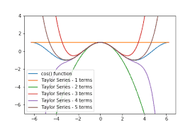
Implicit in the definition of convergence is a simple but very important fact: if $P(a)$ converges, then its value can be approximated by the partial sum $\mathrm{P}{\mathrm{m}}(\mathrm{a})$, and by choosing a sufficiently large value of $m$ we can make the approximation as accurate as we wish. Combining this observation with (2.11), At each point $\mathrm{z}$ in the disc of convergence, $\mathrm{P}(\mathrm{z})$ can be approximated with arbitrarily high precision by a polynomial $\mathrm{P}{\mathrm{m}}(\mathrm{z})$ of sufficiently high degree.
For simplicity’s sake, let us investigate this further in the case that $P(z)$ is centred at the origin. The error $E_m(z)$ at $z$ associated with the approximation $P_m(z)$ can be defined as the distance $E_m(z)=\left|P(z)-P_m(z)\right|$ between the exact answer and the approximation. For a fixed value of $m$, the error $E_m(z)$ will vary as $z$ moves around in the disc of convergence. Clearly, since $E_m(0)=0$, the error will be extremely small if $z$ is close to the origin, but what if $z$ approaches the circle of convergence? The answer depends on the particular power series, but it can happen that the error becomes enormous! [See Ex. 12.] This does not contradict the above result: for any fixed $z$, no matter how close to the circle of convergence, the error $\mathrm{E}_m(z)$ will become arbitrarily small as $m$ tends to infinity.
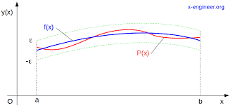
This problem is avoided if we restrict $z$ to the disc $|z| \leqslant r$, where $r<R$, because this prevents $z$ from getting arbitrarily close to the circle of convergence, $|z|=R$. In attempting to approximate $P(z)$ within this disc, it turns out that we can do the following. We first decide on the maximum error (say $\epsilon$ ) that we are willing to put up with, then choose (once and for all) an approximating polynomial $\mathrm{P}_{\mathrm{m}}(z)$ of sufficiently high degree that the error is smaller than $\epsilon$ throughout the disc. That is, throughout the disc, the approximating point $P_m(z)$ lies less than $\epsilon$ away from the true point, $\mathrm{P}(z)$. One describes this by saying that $\mathrm{P}(z)$ is uniformly convergent on this disc:
If $\mathrm{P}(z)$ has disc of convergence $|z|<\mathrm{R}$, then $\mathrm{P}(z)$ is uniformly convergent on the closed disc $|z| \leqslant r$, where $r<R$.
Although we may not have uniform convergence on the whole disc of convergence, the above result shows that this is really a technicality: we do have uniform convergence on a disc that almost fills the complete disc of convergence, say $\mathrm{r}=(0.999999999) \mathrm{R}$.
To verify (2.12), first do Ex. 12, then have a good look at (2.9).
数学代写|复分析作业代写Complex function代考|Uniqueness
If a complex function can be expressed as a power series, then it can only be done so in one way-the power series is unique. This is an immediate consequence of the Identity Theorem:
If
$$
\mathrm{c}0+\mathrm{c}_1 z+\mathrm{c}_2 z^2+\mathrm{c}_3 z^3+\cdots=\mathrm{d}_0+\mathrm{d}_1 z+\mathrm{d}_2 z^2+\mathrm{d}_3 z^3+\cdots $$ for all $z$ in a neighbourhood (no matter how small) of 0 , then the power series are identical: $\mathrm{c}{\mathrm{j}}=\mathrm{d}_{\mathbf{j}}$.
Putting $z=0$ yields $c_0=\mathrm{d}_0$, so they may be cancelled from both sides. Dividing by $z$ and again putting $z=0$ then yields $c_1=d_1$, and so on. [Although this was easy, Ex. 13 shows that it is actually rather remarkable.] The result can be strengthened considerably: If the power series merely agree along a segment of curve (no matter how small) through 0, or if they agree at every point of an infinite sequence of points that converges to 0, then the series are identical. The verification is essentially the same, only instead of putting $z=0$, we now take the limit as $z$ approaches 0 , either along the segment of curve or through the sequence of points.
We can perhaps make greater intuitive sense of these results if we first recall that a power series can be approximated with arbitrarily high precision by a polynomial of sufficiently high degree. Given two points in the plane (no matter how close together) there is a unique line passing through them. Thinking in terms of a graph $y=f(x)$, this says that a polynomial of degree 1 , say $f(x)=c_0+c_1 x$, is uniquely determined by the images of any two points, no matter how close together. Likewise, in the case of degree 2, if we are given three points (no matter how close together), there is only one parabolic graph $y=f(x)=c_0+c_1 x+c_2 x^2$ that can be threaded through them. This idea easily extends to complex functions: there is one, and only one, complex polynomial of degree $n$ that maps a given set of $(n+1)$ points to a given set of $(n+1)$ image points. The above result may therefore be thought of as the limiting case in which the number of known points (together with their known image points) tends to infinity.
Earlier we alluded to a sense in which $h(z)=1 /\left(1+z^2\right)$ is the only complex function that agrees with the real function $H(x)=1 /\left(1+x^2\right)$ on the real line. Yet clearly we can easily write down infinitely many complex functions that agree with $\mathrm{H}(x)$ in this way. For example,
$$
g(z)=g(x+i y)=\frac{\cos \left[x^2 y\right]+i \sin \left[y^2\right]}{e^y+x^2 \ln \left(e+y^4\right)}
$$
Then in what sense can $h(z)$ be considered the unique generalization of $\mathrm{H}(\mathrm{x})$ ?
We already know that $h(z)$ can be expressed as the power series $\sum_{j=0}^{\infty}(-1)^j z^{2 j}$, and this fact yields [exercise] a provisional answer: $h(z)$ is the only complex function that (i) agrees with $\mathrm{H}(\mathrm{x})$ on the real axis, and (ii) can be expressed as a power series in $z$. This still does not completely capture the sense in which $h(z)$ is unique, but it’s a start.
复分析代写
数学代写|复分析作业代写Complex function代考|Approximating a Power Series with a Polynomial
收敛定义中隐含了一个简单但非常重要的事实: 如果 $P(a)$ 收敛,那么它的值可以用部分和来近似 $\operatorname{Pm}(\mathrm{a})$ ,并通过选择足够大的值 $m$ 我们可以使近似值尽可能准确。将此观察结果与 (2.11) 相结合,在 每个点 $z$ 在会聚圆盘中, $\mathrm{P}(\mathrm{z})$ 可以通过多项式以任意高精度近似 $\operatorname{Pm}(\mathrm{z})$ 足够高的程度。
为了简单起见,让我们在以下情况下进一步调查 $P(z)$ 以原点为中心。错误 $E_m(z)$ 在 $z$ 与近似相关 $P_m(z)$ 可以定义为距离 $E_m(z)=\left|P(z)-P_m(z)\right|$ 在准确答案和近似值之间。对于固定值 $m$ ,错误 $E_m(z)$ 会有所不同 $z$ 在会聚圆盘中四处移动。显然,因为 $E_m(0)=0$, 如果 $z$ 接近原点,但如果 $z$ 接近收 敛圆? 答案取决于特定的帋级数,但误差可能会变得很大! [见例。12.] 这与上述结果并不矛盾:对于任 何固定的 $z$ ,无论收敛圆有多接近,误差 $\mathrm{E}m(z)$ 将变得任意小 $m$ 趋于无穷大。 如果我们限制这个问题就可以避免 $z$ 到光盘 $|z| \leqslant r$ ,在哪里 $r{\mathrm{m}}(z)$ 程度足够高,误差小于 $\epsilon$ 整个 光盘。即,在整个圆盘中,逼近点 $P_m(z)$ 小于 $\epsilon$ 远离真实点, $\mathrm{P}(z)$.一个人这样描述这个 $\mathrm{P}(z)$ 在这个圆 盘上一致收敛:
如果 $\mathrm{P}(z)$ 有收敛圆盘 $|z|<\mathrm{R}$ ,然后 $\mathrm{P}(z)$ 一致收敛于闭盘 $|z| \leqslant r$ ,在哪里 $r<R$.
虽然我们可能没有在整个收敛圆盘上一致收敛,但上面的结果表明这确实是一个技术问题: 我们在几乎 填满整个收敛圆盘的圆盘上确实有一致收敛,比如说 $r=(0.999999999) R$. 要验证 (2.12),首先做 Ex. 12,然后好好看看(2.9)。
数学代写|复分析作业代写Complex function代考|Uniqueness
如果一个复杂的函数可以表示为幂级数,那么只能用一种方式来表示一一幂级数是唯一的。这是恒等定 理的直接结果: 如果
$$
\mathrm{c} 0+\mathrm{c}1 z+\mathrm{c}_2 z^2+\mathrm{c}_3 z^3+\cdots=\mathrm{d}_0+\mathrm{d}_1 z+\mathrm{d}_2 z^2+\mathrm{d}_3 z^3+\cdots $$ 对全部 $z$ 在 0 的邻域 (无论多小) 中,幂级数相同: $c j=\mathrm{d}{\mathbf{j}}$.
推杆 $z=0$ 产量 $c_0=\mathrm{d}0$ ,所以他们可能会从双方取消。除以 $z$ 再次投入 $z=0$ 然后产量 $c_1=d_1$ ,等 等。[虽然这很容易,Ex。13 表明它实际上相当显着。] 结果可以大大加强:如果幂级数仅沿着通过 0 的 曲线段 (无论多小) 一致,或者如果它们在无限点序列的每个点都一致收敛于0,则级数相同。验证本质 上是一样的,只是代替了put $z=0$ ,我们现在将极限作为 $z$ 沿着曲线段或通过点序列接近 0 。 如果我们首先回忆起可以通过足够高次数的多项式以任意高精度逼近幂级数,我们或许可以更直观地理 解这些结果。给定平面上的两个点(无论距离多近),有一条唯一的线穿过它们。用图表思考 $y=f(x)$ 同样,在 2 次的情况下,如果给我们三个点(无论多近),则只有一个抛物线图 $y=f(x)=c_0+c_1 x+c_2 x^2$ 可以穿过它们。这个想法很容易扩展到复杂的功能:有一个,而且只有 一个,复杂的次数多项式 $n$ 映射一组给定的 $(n+1)$ 指向一组给定的 $(n+1)$ 图像点。因此,上述结果可 以被认为是已知点 (连同它们的已知图像点) 的数量趋于无穷大的极限情况。 早些时候我们提到了一种感觉 $h(z)=1 /\left(1+z^2\right)$ 是唯一符合实函数的复函数 $H(x)=1 /\left(1+x^2\right)$ 在实线上。然而很明显,我们可以很容易地写出无限多的复杂函数,这些函数符合 $\mathrm{H}(x)$ 这样。例如, $$ g(z)=g(x+i y)=\frac{\cos \left[x^2 y\right]+i \sin \left[y^2\right]}{e^y+x^2 \ln \left(e+y^4\right)} $$ 那么在什么意义上可以 $h(z)$ 被认为是 $\mathrm{H}(\mathrm{x}) ?$ 我们已经知道 $h(z)$ 可以表示为幂级数 $\sum{j=0}^{\infty}(-1)^j z^{2 j}$ ,这个事实产生了[练习]一个临时的答案: $h(z)$ 是 (i) 同意的唯一复杂函数 $\mathrm{H}(\mathrm{x}$ ) 在实轴上,并且 (ii) 可以表示为幂级数 $z$. 这仍然没有完全捕捉到 $h(z)$ 是独一无二的,但这是一个开始。

统计代写请认准statistics-lab™. statistics-lab™为您的留学生涯保驾护航。
金融工程代写
金融工程是使用数学技术来解决金融问题。金融工程使用计算机科学、统计学、经济学和应用数学领域的工具和知识来解决当前的金融问题,以及设计新的和创新的金融产品。
非参数统计代写
非参数统计指的是一种统计方法,其中不假设数据来自于由少数参数决定的规定模型;这种模型的例子包括正态分布模型和线性回归模型。
广义线性模型代考
广义线性模型(GLM)归属统计学领域,是一种应用灵活的线性回归模型。该模型允许因变量的偏差分布有除了正态分布之外的其它分布。
术语 广义线性模型(GLM)通常是指给定连续和/或分类预测因素的连续响应变量的常规线性回归模型。它包括多元线性回归,以及方差分析和方差分析(仅含固定效应)。
有限元方法代写
有限元方法(FEM)是一种流行的方法,用于数值解决工程和数学建模中出现的微分方程。典型的问题领域包括结构分析、传热、流体流动、质量运输和电磁势等传统领域。
有限元是一种通用的数值方法,用于解决两个或三个空间变量的偏微分方程(即一些边界值问题)。为了解决一个问题,有限元将一个大系统细分为更小、更简单的部分,称为有限元。这是通过在空间维度上的特定空间离散化来实现的,它是通过构建对象的网格来实现的:用于求解的数值域,它有有限数量的点。边界值问题的有限元方法表述最终导致一个代数方程组。该方法在域上对未知函数进行逼近。[1] 然后将模拟这些有限元的简单方程组合成一个更大的方程系统,以模拟整个问题。然后,有限元通过变化微积分使相关的误差函数最小化来逼近一个解决方案。
tatistics-lab作为专业的留学生服务机构,多年来已为美国、英国、加拿大、澳洲等留学热门地的学生提供专业的学术服务,包括但不限于Essay代写,Assignment代写,Dissertation代写,Report代写,小组作业代写,Proposal代写,Paper代写,Presentation代写,计算机作业代写,论文修改和润色,网课代做,exam代考等等。写作范围涵盖高中,本科,研究生等海外留学全阶段,辐射金融,经济学,会计学,审计学,管理学等全球99%专业科目。写作团队既有专业英语母语作者,也有海外名校硕博留学生,每位写作老师都拥有过硬的语言能力,专业的学科背景和学术写作经验。我们承诺100%原创,100%专业,100%准时,100%满意。
随机分析代写
随机微积分是数学的一个分支,对随机过程进行操作。它允许为随机过程的积分定义一个关于随机过程的一致的积分理论。这个领域是由日本数学家伊藤清在第二次世界大战期间创建并开始的。
时间序列分析代写
随机过程,是依赖于参数的一组随机变量的全体,参数通常是时间。 随机变量是随机现象的数量表现,其时间序列是一组按照时间发生先后顺序进行排列的数据点序列。通常一组时间序列的时间间隔为一恒定值(如1秒,5分钟,12小时,7天,1年),因此时间序列可以作为离散时间数据进行分析处理。研究时间序列数据的意义在于现实中,往往需要研究某个事物其随时间发展变化的规律。这就需要通过研究该事物过去发展的历史记录,以得到其自身发展的规律。
回归分析代写
多元回归分析渐进(Multiple Regression Analysis Asymptotics)属于计量经济学领域,主要是一种数学上的统计分析方法,可以分析复杂情况下各影响因素的数学关系,在自然科学、社会和经济学等多个领域内应用广泛。
MATLAB代写
MATLAB 是一种用于技术计算的高性能语言。它将计算、可视化和编程集成在一个易于使用的环境中,其中问题和解决方案以熟悉的数学符号表示。典型用途包括:数学和计算算法开发建模、仿真和原型制作数据分析、探索和可视化科学和工程图形应用程序开发,包括图形用户界面构建MATLAB 是一个交互式系统,其基本数据元素是一个不需要维度的数组。这使您可以解决许多技术计算问题,尤其是那些具有矩阵和向量公式的问题,而只需用 C 或 Fortran 等标量非交互式语言编写程序所需的时间的一小部分。MATLAB 名称代表矩阵实验室。MATLAB 最初的编写目的是提供对由 LINPACK 和 EISPACK 项目开发的矩阵软件的轻松访问,这两个项目共同代表了矩阵计算软件的最新技术。MATLAB 经过多年的发展,得到了许多用户的投入。在大学环境中,它是数学、工程和科学入门和高级课程的标准教学工具。在工业领域,MATLAB 是高效研究、开发和分析的首选工具。MATLAB 具有一系列称为工具箱的特定于应用程序的解决方案。对于大多数 MATLAB 用户来说非常重要,工具箱允许您学习和应用专业技术。工具箱是 MATLAB 函数(M 文件)的综合集合,可扩展 MATLAB 环境以解决特定类别的问题。可用工具箱的领域包括信号处理、控制系统、神经网络、模糊逻辑、小波、仿真等。