如果你也在 怎样代写复分析Complex function这个学科遇到相关的难题,请随时右上角联系我们的24/7代写客服。
复分析是一个从复数到复数的函数。换句话说,它是一个以复数的一个子集为域,以复数为子域的函数。复数函数通常应该有一个包含复数平面的非空开放子集的域。
statistics-lab™ 为您的留学生涯保驾护航 在代写复分析Complex function方面已经树立了自己的口碑, 保证靠谱, 高质且原创的统计Statistics代写服务。我们的专家在代写复分析Complex function代写方面经验极为丰富,各种代写复分析Complex function相关的作业也就用不着说。
我们提供的复分析Complex function及其相关学科的代写,服务范围广, 其中包括但不限于:
- Statistical Inference 统计推断
- Statistical Computing 统计计算
- Advanced Probability Theory 高等概率论
- Advanced Mathematical Statistics 高等数理统计学
- (Generalized) Linear Models 广义线性模型
- Statistical Machine Learning 统计机器学习
- Longitudinal Data Analysis 纵向数据分析
- Foundations of Data Science 数据科学基础
数学代写|复分析作业代写Complex function代考|The Explanation: Homogeneous Coordinates
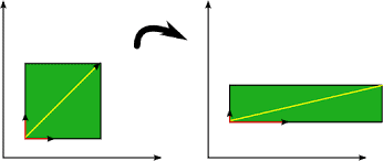
Clearly this cannot all be coincidence, but what is really going on here?! The answer is simple, yet subtle. To see it we must first describe the complex plane with a completely new kind of coordinate system. Instead of expressing $z=x+i y$ in terms of two real numbers, we write it as the ratio of two complex numbers, $z_1$ and $\mathfrak{z}2$ : $$ z=\frac{z_1}{z_2} $$ The ordered pair of complex numbers $\left[z_1, z_2\right]$ are called homogeneous coordinates of $z$. In order that this ratio be well defined we demand that $\left[z_1, z_2\right] \neq[0,0]$. To each ordered pair $\left[\mathfrak{z}_1\right.$ arbitrary, $\left.\mathfrak{z}_2 \neq 0\right]$ there corresponds precisely one point $z=\left(\mathfrak{z}_1 / \mathfrak{z}_2\right)$, but to each point $z$ there corresponds an infinite set of homogeneous coordinates, $\left[\mathrm{k}{z_1}, \mathrm{k}_{z_2}\right]=\mathrm{k}\left[z_1, \mathfrak{z}_2\right]$, where $\mathrm{k}$ is an arbitrary non-zero complex number.
What about a pair of the form $\left[z_1, 0\right]$ ? By holding $z_1$ fixed as $z_2$ tends to 0 , it is clear that $\left[z_1, 0\right]$ must be identified with the point at infinity. Thus the totality of pairs $\left[z_1, z_2\right]$ provide coordinates for the extended complex plane. The introduction of homogeneous coordinates thereby accomplishes for algebra what the Riemann sphere accomplishes for geometry-it does away with the exceptional role of $\infty$.
Just as we use the symbol $\mathbb{R}^2$ to denote the set of pairs $(x, y)$ of real numbers, so we use the symbol $\mathbb{C}^2$ to denote the set of pairs $\left[\mathfrak{z}_1, \mathfrak{z}_2\right]$ of complex numbers. To highlight the distinction between $\mathbb{R}^2$ and $\mathbb{C}^2$, we use conventional round brackets when writing down an element $(x, y)$ of $\mathbb{R}^2$, but we use square brackets for an element $\left[z_1, z_2\right]$ of $\mathbb{C}^2$.
Just as a linear transformation of $\mathbb{R}^2$ is represented by a real $2 \times 2$ matrix, so a linear transformation of $\mathbb{C}^2$ is represented by a complex $2 \times 2$ matrix:
$$
\left[\begin{array}{l}
z_1 \
\mathfrak{z}2 \end{array}\right] \longmapsto\left[\begin{array}{l} \mathfrak{w}_1 \ \mathfrak{w}_2 \end{array}\right]=\left[\begin{array}{ll} a & b \ c & d \end{array}\right]\left[\begin{array}{l} z_1 \ \mathfrak{z}_2 \end{array}\right]=\left[\begin{array}{l} a \mathfrak{z}_1+b{z_2} \
\mathrm{c} \mathfrak{z}1+d{z_2}
\end{array}\right] .
$$
But if $\left[\mathfrak{z}1, \mathfrak{z}_2\right]$ and $\left[\mathfrak{w}_1, \mathfrak{w}_2\right]$ are thought of as the homogeneous coordinates in $\mathbb{C}^2$ of the point $z=\left(\mathfrak{z}_1 / \mathfrak{z}_2\right)$ in $\mathbb{C}$ and its image point $w=\left(\mathfrak{w}_1 / \mathfrak{w}_2\right)$, then the above linear transformation of $\mathbb{C}^2$ induces the following (non-linear) transformation of $\mathbb{C}$ : $$ z=\frac{\mathfrak{z}_1}{\mathfrak{z}_2} \longmapsto w=\frac{\mathfrak{w}_1}{\mathfrak{w}_2}=\frac{a \mathfrak{z}_1+b{\mathfrak{z}2}}{\mathrm{c} \mathfrak{z}_1+\mathrm{d}{\mathfrak{z}_2}}=\frac{\mathrm{a}\left(\mathfrak{z}_1 / \mathfrak{z}_2\right)+b}{\mathrm{c}\left(\mathfrak{z}_1 / \mathfrak{z}_2\right)+d}=\frac{a z+b}{c z+d} .
$$
数学代写|复分析作业代写Complex function代考|Eigenvectors and Eigenvalues
The above representation of Möbius transformations as matrices provides an elegant and practical method of doing concrete calculations. More significantly, however, it also means that in developing the theory of Möbius transformations we suddenly have access to a whole range of new ideas and techniques taken from linear algebra.
We begin with something very simple. We previously remarked that while it is geometrically obvious that the composition of two non-singular Möbius transformations is again non-singular, it is far from obvious algebraically. Our new point of view rectifies this, for recall the following elementary property of determinants:
$$
\operatorname{det}\left{\left[M_2\right]\left[M_1\right]\right}=\operatorname{det}\left[M_2\right] \operatorname{det}\left[M_1\right]
$$
Thus if $\operatorname{det}\left[M_2\right] \neq 0$ and $\operatorname{det}\left[M_1\right] \neq 0$, then $\operatorname{det}\left[\left[M_2\right]\left[M_1\right]\right} \neq 0$, as was to be shown. This also sheds further light on the virtue of working with normalized Möbius transformations. For if $\operatorname{det}\left[M_2\right]=1$ and $\operatorname{det}\left[M_1\right]=1$, then $\operatorname{det}\left{\left[M_2\right]\left[M_1\right]\right}=1$. Thus the set of normalized $2 \times 2$ matrices form a group-a “subgroup” of the full group of non-singular matrices.
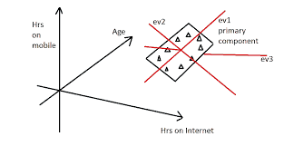
For our second example, consider the eigenvectors of a linear transformation $[M]=\left[\begin{array}{ll}a & b \ c & d\end{array}\right]$ of $\mathbb{C}^2$. By definition, an eigenvector is a vector $\mathfrak{z}=\left[\begin{array}{l}\mathfrak{z}1 \ \mathfrak{z}_2\end{array}\right]$ whose “direction” is unaltered by the transformation, in the sense that its image is simply a multiple $\lambda_z$ of the original; this multiple $\lambda$ is called the eigenvalue of the eigenvector. In other words, an eigenvector satisfies the equation $$ \left[\begin{array}{ll} a & b \ c & d \end{array}\right]\left[\begin{array}{l} z_1 \ z_2 \end{array}\right]=\lambda\left[\begin{array}{l} z_1 \ \mathfrak{z}_2 \end{array}\right] $$ In terms of the corresponding Möbius transformation in $\mathbb{C}$, this means that $z=$ $\left(z_1 / z_2\right)$ is mapped to $M(z)=\left(\lambda{z_1} / \lambda_{z_2}\right)=z$, and so
$z=\left(z_1 / z_2\right)$ is a fixed point of $\mathrm{M}(z)$ if and only if $z=\left[\begin{array}{l}z_1 \ z_2\end{array}\right]$ is an eigenvector of $[\mathrm{M}]$.
Note that one immediate benefit of this approach is that there is no longer any real distinction between a finite fixed point and a fixed point at $\infty$, for the latter merely corresponds to an eigenvector of the form $\left[\begin{array}{c}z_1 \ 0\end{array}\right]$.
复分析代写
数学代写|复分析作业代写Complex function代考|The Explanation: Homogeneous Coordinates
显然这不可能都是巧合,但这到底是怎么回事? !答案很简单,但很微妙。要看到它,我们必须首先用一 种全新的坐标系来描述复平面。而不是表达 $z=x+i y$ 就两个实数而言,我们将其写为两个复数之比, $z_1$ 和 $z 2$ :
$$
z=\frac{z_1}{z_2}
$$
有序复数对 $\left[z_1, z_2\right]$ 称为齐次坐标 $z$. 为了明确定义这个比率,我们要求 $\left[z_1, z_2\right] \neq[0,0]$. 对于每个有序对 $\left[\mathfrak{z}1\right.$ 随意的, $\left.z_2 \neq 0\right]$ 正好对应一点 $z=\left(z_1 / z_2\right)$ ,但对每个点 $z$ 对应于无限组齐次坐标, $\left[\mathrm{k} z_1, \mathrm{k}{z_2}\right]=\mathrm{k}\left[z_1, z_2\right]$ , 在哪里 $\mathrm{k}$ 是任意非零复数。
一对表格怎么样 $\left[z_1, 0\right]$ ? 通过持有 $z_1$ 固定为 $z_2$ 趋于 0 ,显然 $\left[z_1, 0\right]$ 必须等同于无穷远点。因此对的总数 $\left[z_1, z_2\right]$ 为扩展复平面提供坐标。引入齐次坐标从而为代数完成了黎曼球为几何所完成的工作一一它消除 了特殊的作用 .
正如我们使用符号 $\mathbb{R}^2$ 表示对的集合 $(x, y)$ 的实数,所以我们使用符号 $\mathbb{C}^2$ 表示对的集合 $\left[\mathfrak{z}1, \mathfrak{z}_2\right]$ 的复数。为 了突出两者之间的区别 $\mathbb{R}^2$ 和 $\mathbb{C}^2$ ,我们在写下一个元素时使用传统的圆括号 $(x, y)$ 的 $\mathbb{R}^2$ ,但我们对元素使 用方括号 $\left[z_1, z_2\right]$ 的 $\mathbb{C}^2$. 正如线性变换 $\mathbb{R}^2$ 由一个真实的代表 $2 \times 2$ 矩阵,所以线性变换 $\mathbb{C}^2$ 由一个复杂的表示 $2 \times 2$ 矩阵: $$ \left[\begin{array}{ll} z_1 & \mathfrak{z}^2 \end{array}\right] \longmapsto\left[\mathfrak{w}_1 \mathfrak{w}_2\right]=\left[\begin{array}{lll} a & b c & d \end{array}\right]\left[z_1 \mathfrak{z}_2\right]=\left[a{\mathfrak{z}1}+b z_2 \mathfrak{c}{\mathfrak{z}} 1+d z_2\right] .
$$
但是如果 $\left[\mathfrak{z}^1, \mathfrak{z}2\right]$ 和 $\left[\mathfrak{w}_1, \mathfrak{w}_2\right]$ 被认为是齐次坐标 $\mathbb{C}^2$ 重点 $z=\left(\mathfrak{z}_1 / \mathfrak{z}_2\right)$ 在 $\mathbb{C}$ 及其像点 $w=\left(\mathfrak{w}_1 / \mathfrak{w}_2\right)$ ,那么 上面的线性变换 $\mathbb{C}^2$ 引起以下 (非线性) 变换 $\mathbb{C}$ : $$ z=\frac{\mathfrak{z}_1}{\mathfrak{z}_2} \longmapsto w=\frac{\mathfrak{w}_1}{\mathfrak{w}_2}=\frac{a{\mathfrak{z}1}+b{\mathfrak{z}} 2}{\mathrm{c}{\mathfrak{z}_1}+\mathrm{d}{\mathfrak{z}_2}}=\frac{\mathrm{a}\left(\mathfrak{z}_1 / \mathfrak{z}_2\right)+b}{\mathrm{c}\left(\mathfrak{z}_1 / \mathfrak{z}_2\right)+d}=\frac{a z+b}{c z+d}
$$
数学代写|复分析作业代写Complex function代考|Eigenvectors and Eigenvalues
上面将莫比乌斯变换表示为矩阵,提供了一种优雅实用的具体计算方法。然而,更重要的是,这也意味着 在发展莫比乌斯变换理论的过程中,我们突然可以接触到从线性代数中提取的一系列新思想和新技术。
我们从非常简单的事情开始。我们之前说过,虽然两个非奇异莫比乌斯变换的组合在几何上也是非奇异 的,但在代数上远非如此。我们的新观点纠正了这一点,回想一下行列式的以下基本性质:
因此,如果 $\operatorname{det}\left[M_2\right] \neq 0$ 和 $\operatorname{det}\left[M_1\right] \neq 0 \mathrm{~ , 然 后 ~}$ 了使用标准化莫比乌斯变换的优点。对于如果 $\operatorname{det}\left[M_2\right]=1$ 和det $\left[M_1\right]=1 \mathrm{~ , 然 后 ~}$ 群一一非奇异矩阵全群的一个”子群”。
对于我们的第二个例子,考虑线性变换的特征向量 $[M]=\left[\begin{array}{lll}a & b c & d\end{array}\right]$ 的 $\mathbb{C}^2$. 根据定义,特征向量是一 个向量 $\mathfrak{z}=\left[{ }^z 1 \mathfrak{z}2\right]$ 其“方向”末因变换而改变,从某种意义上说,它的图像只是一个倍数 $\lambda_z$ 原件;这个倍 数 $\lambda$ 称为特征向量的特征值。换句话说,特征向量满足方程 $$ \left[\begin{array}{lll} a & b c & d \end{array}\right]\left[\begin{array}{ll} z_1 & z_2 \end{array}\right]=\lambda\left[\begin{array}{ll} z_1 & z_2 \end{array}\right] $$ 根据相应的莫比乌斯变换 $\mathbb{C}$ ,这意味着 $z=\left(z_1 / z_2\right)$ 映射到 $M(z)=\left(\lambda z_1 / \lambda{z_2}\right)=z$ ,所以 $z=\left(z_1 / z_2\right)$ 是一个不动点 $\mathrm{M}(z)$ 当且仅当 $z=\left[\begin{array}{ll}z_1 & z_2\end{array}\right]$ 是的特征向量 $[\mathrm{M}]$.
请注意,这种方法的一个直接好处是,有限不动点和处的不动点之间不再有任何真正的区别。 $\infty ,$ 因为 后者仅对应于以下形式的特征向量 $\left[\begin{array}{ll}z_1 & 0\end{array}\right]$.

统计代写请认准statistics-lab™. statistics-lab™为您的留学生涯保驾护航。
金融工程代写
金融工程是使用数学技术来解决金融问题。金融工程使用计算机科学、统计学、经济学和应用数学领域的工具和知识来解决当前的金融问题,以及设计新的和创新的金融产品。
非参数统计代写
非参数统计指的是一种统计方法,其中不假设数据来自于由少数参数决定的规定模型;这种模型的例子包括正态分布模型和线性回归模型。
广义线性模型代考
广义线性模型(GLM)归属统计学领域,是一种应用灵活的线性回归模型。该模型允许因变量的偏差分布有除了正态分布之外的其它分布。
术语 广义线性模型(GLM)通常是指给定连续和/或分类预测因素的连续响应变量的常规线性回归模型。它包括多元线性回归,以及方差分析和方差分析(仅含固定效应)。
有限元方法代写
有限元方法(FEM)是一种流行的方法,用于数值解决工程和数学建模中出现的微分方程。典型的问题领域包括结构分析、传热、流体流动、质量运输和电磁势等传统领域。
有限元是一种通用的数值方法,用于解决两个或三个空间变量的偏微分方程(即一些边界值问题)。为了解决一个问题,有限元将一个大系统细分为更小、更简单的部分,称为有限元。这是通过在空间维度上的特定空间离散化来实现的,它是通过构建对象的网格来实现的:用于求解的数值域,它有有限数量的点。边界值问题的有限元方法表述最终导致一个代数方程组。该方法在域上对未知函数进行逼近。[1] 然后将模拟这些有限元的简单方程组合成一个更大的方程系统,以模拟整个问题。然后,有限元通过变化微积分使相关的误差函数最小化来逼近一个解决方案。
tatistics-lab作为专业的留学生服务机构,多年来已为美国、英国、加拿大、澳洲等留学热门地的学生提供专业的学术服务,包括但不限于Essay代写,Assignment代写,Dissertation代写,Report代写,小组作业代写,Proposal代写,Paper代写,Presentation代写,计算机作业代写,论文修改和润色,网课代做,exam代考等等。写作范围涵盖高中,本科,研究生等海外留学全阶段,辐射金融,经济学,会计学,审计学,管理学等全球99%专业科目。写作团队既有专业英语母语作者,也有海外名校硕博留学生,每位写作老师都拥有过硬的语言能力,专业的学科背景和学术写作经验。我们承诺100%原创,100%专业,100%准时,100%满意。
随机分析代写
随机微积分是数学的一个分支,对随机过程进行操作。它允许为随机过程的积分定义一个关于随机过程的一致的积分理论。这个领域是由日本数学家伊藤清在第二次世界大战期间创建并开始的。
时间序列分析代写
随机过程,是依赖于参数的一组随机变量的全体,参数通常是时间。 随机变量是随机现象的数量表现,其时间序列是一组按照时间发生先后顺序进行排列的数据点序列。通常一组时间序列的时间间隔为一恒定值(如1秒,5分钟,12小时,7天,1年),因此时间序列可以作为离散时间数据进行分析处理。研究时间序列数据的意义在于现实中,往往需要研究某个事物其随时间发展变化的规律。这就需要通过研究该事物过去发展的历史记录,以得到其自身发展的规律。
回归分析代写
多元回归分析渐进(Multiple Regression Analysis Asymptotics)属于计量经济学领域,主要是一种数学上的统计分析方法,可以分析复杂情况下各影响因素的数学关系,在自然科学、社会和经济学等多个领域内应用广泛。
MATLAB代写
MATLAB 是一种用于技术计算的高性能语言。它将计算、可视化和编程集成在一个易于使用的环境中,其中问题和解决方案以熟悉的数学符号表示。典型用途包括:数学和计算算法开发建模、仿真和原型制作数据分析、探索和可视化科学和工程图形应用程序开发,包括图形用户界面构建MATLAB 是一个交互式系统,其基本数据元素是一个不需要维度的数组。这使您可以解决许多技术计算问题,尤其是那些具有矩阵和向量公式的问题,而只需用 C 或 Fortran 等标量非交互式语言编写程序所需的时间的一小部分。MATLAB 名称代表矩阵实验室。MATLAB 最初的编写目的是提供对由 LINPACK 和 EISPACK 项目开发的矩阵软件的轻松访问,这两个项目共同代表了矩阵计算软件的最新技术。MATLAB 经过多年的发展,得到了许多用户的投入。在大学环境中,它是数学、工程和科学入门和高级课程的标准教学工具。在工业领域,MATLAB 是高效研究、开发和分析的首选工具。MATLAB 具有一系列称为工具箱的特定于应用程序的解决方案。对于大多数 MATLAB 用户来说非常重要,工具箱允许您学习和应用专业技术。工具箱是 MATLAB 函数(M 文件)的综合集合,可扩展 MATLAB 环境以解决特定类别的问题。可用工具箱的领域包括信号处理、控制系统、神经网络、模糊逻辑、小波、仿真等。