如果你也在 怎样代写凸优化Convex optimization 这个学科遇到相关的难题,请随时右上角联系我们的24/7代写客服。凸优化Convex optimization凸优化是数学优化的一个子领域,研究的是凸集上凸函数最小化的问题。许多类凸优化问题允许采用多项式时间算法,而数学优化一般来说是NP-hard。
凸优化Convex optimization是数学优化的一个子领域,研究的是凸集上凸函数最小化的问题。许多类别的凸优化问题允许采用多项式时间算法,而数学优化一般来说是NP困难的。凸优化在许多学科中都有应用,如自动控制系统、估计和信号处理、通信和网络、电子电路设计、数据分析和建模、金融、统计(最佳实验设计)、和结构优化,其中近似概念被证明是有效的。
statistics-lab™ 为您的留学生涯保驾护航 在代写凸优化Convex Optimization方面已经树立了自己的口碑, 保证靠谱, 高质且原创的统计Statistics代写服务。我们的专家在代写凸优化Convex Optimization代写方面经验极为丰富,各种代写凸优化Convex Optimization相关的作业也就用不着说。
数学代写|凸优化作业代写Convex Optimization代考|Conjugate Gradient Methods
There is an interesting connection between the extrapolation method $(2.12)$ and the conjugate gradient method for unconstrained differentiable optimization. This is a classical method, with an extensive theory, and the distinctive property that it minimizes an $n$-dimensional convex quadratic cost function in at most $n$ iterations, each involving a single line minimization. Fast progress is often obtained in much less than $n$ iterations, depending on the eigenvalue structure of the quadratic cost [see e.g., [Ber82a] (Section 1.3.4), or [Lue84] (Chapter 8)]. The method can be implemented in several different ways, for which we refer to textbooks such as [Lue84], [Ber99]. It is a member of the more general class of conjugate direction methods, which involve a sequence of exact line searches along directions that are orthogonal with respect to some generalized inner product.
It turns out that if the parameters $\alpha_k$ and $\beta_k$ in iteration (2.12) are chosen optimally for each $k$ so that
$$
\left(\alpha_k, \beta_k\right) \in \arg \min {\alpha \in \Re, \beta \in \Re} f\left(x_k-\alpha \nabla f\left(x_k\right)+\beta\left(x_k-x{k-1}\right)\right), \quad k=0,1, \ldots,
$$
with $x_{-1}=x_0$, the resulting method is an implementation of the conjugate gradient method (see e.g., [Ber99], Section 1.6). By this we mean that if $f$ is a convex quadratic function, the method (2.12) with the stepsize choice (2.13) generates exactly the same iterates as the conjugate gradient method, and hence minimizes $f$ in at most $n$ iterations. Finding the optimal parameters according to Eq. (2.13) requires solution of a two-dimensional optimization problem in $\alpha$ and $\beta$, which may be impractical in the absence of special structure. However, this optimization is facilitated in some important special cases, which also favor the use of other types of conjugate direction methods. $\dagger$
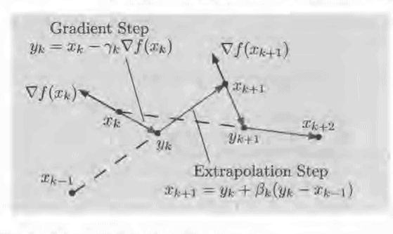
There are several other ways to implement the conjugate gradient method, all of which generate identical iterates for quadratic cost functions, but may differ substantially in their behavior for nonquadratic ones. One of them, which resembles the preceding extrapolation methods, is the method of parallel tangents or PARTAN, first proposed in the paper [SBK64]. In particular, each iteration of PARTAN involves extrapolation and two onedimensional line minimizations. At the typical iteration, given $x_k$, we obtain $x_{k+1}$ as follows:
(1) We find a vector $y_k$ that minimizes $f$ over the line
$$
\left{y=x_k-\gamma \nabla f\left(x_k\right) \mid \gamma \geq 0\right} .
$$
数学代写|凸优化作业代写Convex Optimization代考|Newton’s Method
In Newton’s method the descent direction is
$$
d_k=-\left(\nabla^2 f\left(x_k\right)\right)^{-1} \nabla f\left(x_k\right),
$$
provided $\nabla^2 f\left(x_k\right)$ exists and is positive definite, so the iteration takes the form
$$
x_{k+1}=x_k-\alpha_k\left(\nabla^2 f\left(x_k\right)\right)^{-1} \nabla f\left(x_k\right) .
$$
If $\nabla^2 f\left(x_k\right)$ is not positive definite, some modification is necessary. There are several possible modifications of this type, for which the reader may consult nonlinear programming textbooks. The simplest one is to add to $\nabla^2 f\left(x_k\right)$ a small positive multiple of the identity. Generally, when $f$ is convex, $\nabla^2 f\left(x_k\right)$ is positive semidefinite (Prop. 1.1.10 in Appendix B), and this facilitates the implementation of reliable Newton-type algorithms.
The idea in Newton’s method is to minimize at each iteration the quadratic approximation of $f$ around the current point $x_k$ given by
$$
\tilde{f}k(x)=f\left(x_k\right)+\nabla f\left(x_k\right)^{\prime}\left(x-x_k\right)+\frac{1}{2}\left(x-x_k\right)^{\prime} \nabla^2 f\left(x_k\right)\left(x-x_k\right) . $$ By setting the gradient of $\tilde{f}_k(x)$ to zero, $$ \nabla f\left(x_k\right)+\nabla^2 f\left(x_k\right)\left(x-x_k\right)=0 $$ and solving for $x$, we obtain as next iterate the minimizing point $$ x{k+1}=x_k-\left(\nabla^2 f\left(x_k\right)\right)^{-1} \nabla f\left(x_k\right) \text {. }
$$
This is the Newton iteration corresponding to a stepsize $\alpha_k=1$. It follows that, assuming $\alpha_k=1$, Newton’s method finds the global minimum of a positive definite quadratic function in a single iteration.
Newton’s method typically converges very fast asymptotically, assuming that it converges to a vector $x^$ such that $\nabla f\left(x^\right)=0$ and $\nabla^2 f\left(x^*\right)$is positive definite, and that a stepsize $\alpha_k=1$ is used, at least after some iteration. For a simple argument, we may use Taylor’s theorem to write
$$
0=\nabla f\left(x^\right)=\nabla f\left(x_k\right)+\nabla^2 f\left(x_k\right)^{\prime}\left(x^-x_k\right)+o\left(\left|x_k-x^\right|\right) . $$ By multiplying this relation with $\left(\nabla^2 f\left(x_k\right)\right)^{-1}$ we have $$ x_k-x^-\left(\nabla^2 f\left(x_k\right)\right)^{-1} \nabla f\left(x_k\right)=o\left(\left|x_k-x^\right|\right), $$ so for the Newton iteration with stepsize $\alpha_k=1$ we obtain $$ x_{k+1}-x^=o\left(\left|x_k-x^\right|\right) $$ or, for $x_k \neq x^$,
$$
\lim {k \rightarrow \infty} \frac{\left|x{k+1}-x^\right|}{\left|x_k-x^\right|}=\lim _{k \rightarrow \infty} \frac{o\left(\left|x_k-x^\right|\right)}{\left|x_k-x^\right|}=0,
$$
implying convergence that is faster than linear (also called superlinear). This argument can also be used to show local convergence to $x^$ with $\alpha_k \equiv 1$, that is convergence assuming that $x_0$ is sufficiently close to $x^$.

凸优化代写
数学代写|凸优化作业代写Convex Optimization代考|Conjugate Gradient Methods
无约束可微优化的外推方法$(2.12)$与共轭梯度法之间有一个有趣的联系。这是一个经典的方法,具有广泛的理论和独特的性质,它最小化$n$维凸二次代价函数最多$n$迭代,每次涉及单线最小化。快速进展通常在少于$n$次迭代中获得,这取决于二次代价的特征值结构[例如,Ber82a或Lue84]。该方法可以通过几种不同的方式实现,我们参考了[Lue84], [Ber99]等教科书。它是更一般的一类共轭方向方法的一员,它涉及沿着与某些广义内积正交的方向的精确直线搜索序列。
事实证明,如果在迭代(2.12)中为每个$k$选择参数$\alpha_k$和$\beta_k$,那么
$$
\left(\alpha_k, \beta_k\right) \in \arg \min {\alpha \in \Re, \beta\ in \Re} f\left(x_k-\alpha \nabla f\left(x_k\right)+\beta\left(x_k-x{k-1}\right)\right), \quad k=0,1, \ldots,
$$
对于$x_{-1}=x_0$,得到的方法是共轭梯度法的一个实现(例如,[Ber99],第1.6节)。我们的意思是,如果$f$是一个凸二次函数,具有步长选择(2.13)的方法(2.12)与共轭梯度方法产生完全相同的迭代,因此在最多$n$迭代中最小化$f$。根据式(2.13)找到最优参数需要求解$\alpha$和$\beta$中的二维优化问题,在没有特殊结构的情况下,这可能是不切实际的。然而,在一些重要的特殊情况下,这种优化是容易的,这也有利于使用其他类型的共轭方向方法。\匕首美元
还有其他几种实现共轭梯度法的方法,所有这些方法都对二次代价函数产生相同的迭代,但对非二次代价函数的行为可能有很大的不同。其中一种方法类似于前面的外推方法,即平行切线法或PARTAN法,该方法最早由论文[SBK64]提出。特别是,PARTAN的每次迭代都涉及外推和两个一维线最小化。在典型迭代中,给定$x_k$,我们得到$x_{k+1}$如下所示:
(1)我们找到一个向量y_k使f在直线上最小
$$
\left{y=x_k-\gamma \nabla f\left(x_k\right) \mid \gamma \geq 0\right}。
$$
数学代写|凸优化作业代写Convex Optimization代考|Newton’s Method
在牛顿法中,下降方向是
$$
d_k=-\left(\nabla^2 f\left(x_k\right)\right)^{-1} \nabla f\left(x_k\right),
$$
假设$\nabla^2 f\left(x_k\right)$存在并且是正定的,所以迭代采用如下形式
$$
x_{k+1}=x_k-\alpha_k\left(\nabla^2 f\left(x_k\right)\right)^{-1} \nabla f\left(x_k\right) .
$$
如果$\nabla^2 f\left(x_k\right)$不是肯定的,一些修改是必要的。这种类型有几种可能的修改,读者可以参考非线性规划教科书。最简单的方法是给$\nabla^2 f\left(x_k\right)$加上一个单位的小正倍数。一般情况下,当$f$为凸时,$\nabla^2 f\left(x_k\right)$为正半定(见附录B 1.1.10 Prop. 1.1.10),这有利于实现可靠的牛顿型算法。
牛顿方法的思想是在每次迭代中最小化$f$在当前点$x_k$周围的二次逼近
$$
\tilde{f}k(x)=f\left(x_k\right)+\nabla f\left(x_k\right)^{\prime}\left(x-x_k\right)+\frac{1}{2}\left(x-x_k\right)^{\prime} \nabla^2 f\left(x_k\right)\left(x-x_k\right) . $$通过设置$\tilde{f}_k(x)$的梯度为0,$$ \nabla f\left(x_k\right)+\nabla^2 f\left(x_k\right)\left(x-x_k\right)=0 $$并求解$x$,我们得到下一次迭代的最小点 $$ x{k+1}=x_k-\left(\nabla^2 f\left(x_k\right)\right)^{-1} \nabla f\left(x_k\right) \text {. }
$$
这是牛顿迭代对应于步长$\alpha_k=1$。由此可见,假设$\alpha_k=1$,牛顿法在一次迭代中找到一个正定二次函数的全局最小值。
牛顿的方法通常收敛得非常快,假设它收敛于一个向量 $x^$ 这样 $\nabla f\left(x^\right)=0$ 和 $\nabla^2 f\left(x^*\right)$是正的,这是一个步长 $\alpha_k=1$ 至少在一些迭代之后使用。对于一个简单的论证,我们可以用泰勒定理来写
$$
0=\nabla f\left(x^\right)=\nabla f\left(x_k\right)+\nabla^2 f\left(x_k\right)^{\prime}\left(x^-x_k\right)+o\left(\left|x_k-x^\right|\right) . $$ 将这个关系乘以 $\left(\nabla^2 f\left(x_k\right)\right)^{-1}$ 我们有 $$ x_k-x^-\left(\nabla^2 f\left(x_k\right)\right)^{-1} \nabla f\left(x_k\right)=o\left(\left|x_k-x^\right|\right), $$ 对于步长为步长的牛顿迭代 $\alpha_k=1$ 我们得到 $$ x_{k+1}-x^=o\left(\left|x_k-x^\right|\right) $$ 或者,for $x_k \neq x^$,
$$
\lim {k \rightarrow \infty} \frac{\left|x{k+1}-x^\right|}{\left|x_k-x^\right|}=\lim _{k \rightarrow \infty} \frac{o\left(\left|x_k-x^\right|\right)}{\left|x_k-x^\right|}=0,
$$
意味着比线性更快的收敛(也称为超线性)。这个论证也可以用来证明局部收敛 $x^$ 有 $\alpha_k \equiv 1$,这就是收敛假设 $x_0$ 足够接近 $x^$.

统计代写请认准statistics-lab™. statistics-lab™为您的留学生涯保驾护航。
金融工程代写
金融工程是使用数学技术来解决金融问题。金融工程使用计算机科学、统计学、经济学和应用数学领域的工具和知识来解决当前的金融问题,以及设计新的和创新的金融产品。
非参数统计代写
非参数统计指的是一种统计方法,其中不假设数据来自于由少数参数决定的规定模型;这种模型的例子包括正态分布模型和线性回归模型。
广义线性模型代考
广义线性模型(GLM)归属统计学领域,是一种应用灵活的线性回归模型。该模型允许因变量的偏差分布有除了正态分布之外的其它分布。
术语 广义线性模型(GLM)通常是指给定连续和/或分类预测因素的连续响应变量的常规线性回归模型。它包括多元线性回归,以及方差分析和方差分析(仅含固定效应)。
有限元方法代写
有限元方法(FEM)是一种流行的方法,用于数值解决工程和数学建模中出现的微分方程。典型的问题领域包括结构分析、传热、流体流动、质量运输和电磁势等传统领域。
有限元是一种通用的数值方法,用于解决两个或三个空间变量的偏微分方程(即一些边界值问题)。为了解决一个问题,有限元将一个大系统细分为更小、更简单的部分,称为有限元。这是通过在空间维度上的特定空间离散化来实现的,它是通过构建对象的网格来实现的:用于求解的数值域,它有有限数量的点。边界值问题的有限元方法表述最终导致一个代数方程组。该方法在域上对未知函数进行逼近。[1] 然后将模拟这些有限元的简单方程组合成一个更大的方程系统,以模拟整个问题。然后,有限元通过变化微积分使相关的误差函数最小化来逼近一个解决方案。
tatistics-lab作为专业的留学生服务机构,多年来已为美国、英国、加拿大、澳洲等留学热门地的学生提供专业的学术服务,包括但不限于Essay代写,Assignment代写,Dissertation代写,Report代写,小组作业代写,Proposal代写,Paper代写,Presentation代写,计算机作业代写,论文修改和润色,网课代做,exam代考等等。写作范围涵盖高中,本科,研究生等海外留学全阶段,辐射金融,经济学,会计学,审计学,管理学等全球99%专业科目。写作团队既有专业英语母语作者,也有海外名校硕博留学生,每位写作老师都拥有过硬的语言能力,专业的学科背景和学术写作经验。我们承诺100%原创,100%专业,100%准时,100%满意。
随机分析代写
随机微积分是数学的一个分支,对随机过程进行操作。它允许为随机过程的积分定义一个关于随机过程的一致的积分理论。这个领域是由日本数学家伊藤清在第二次世界大战期间创建并开始的。
时间序列分析代写
随机过程,是依赖于参数的一组随机变量的全体,参数通常是时间。 随机变量是随机现象的数量表现,其时间序列是一组按照时间发生先后顺序进行排列的数据点序列。通常一组时间序列的时间间隔为一恒定值(如1秒,5分钟,12小时,7天,1年),因此时间序列可以作为离散时间数据进行分析处理。研究时间序列数据的意义在于现实中,往往需要研究某个事物其随时间发展变化的规律。这就需要通过研究该事物过去发展的历史记录,以得到其自身发展的规律。
回归分析代写
多元回归分析渐进(Multiple Regression Analysis Asymptotics)属于计量经济学领域,主要是一种数学上的统计分析方法,可以分析复杂情况下各影响因素的数学关系,在自然科学、社会和经济学等多个领域内应用广泛。
MATLAB代写
MATLAB 是一种用于技术计算的高性能语言。它将计算、可视化和编程集成在一个易于使用的环境中,其中问题和解决方案以熟悉的数学符号表示。典型用途包括:数学和计算算法开发建模、仿真和原型制作数据分析、探索和可视化科学和工程图形应用程序开发,包括图形用户界面构建MATLAB 是一个交互式系统,其基本数据元素是一个不需要维度的数组。这使您可以解决许多技术计算问题,尤其是那些具有矩阵和向量公式的问题,而只需用 C 或 Fortran 等标量非交互式语言编写程序所需的时间的一小部分。MATLAB 名称代表矩阵实验室。MATLAB 最初的编写目的是提供对由 LINPACK 和 EISPACK 项目开发的矩阵软件的轻松访问,这两个项目共同代表了矩阵计算软件的最新技术。MATLAB 经过多年的发展,得到了许多用户的投入。在大学环境中,它是数学、工程和科学入门和高级课程的标准教学工具。在工业领域,MATLAB 是高效研究、开发和分析的首选工具。MATLAB 具有一系列称为工具箱的特定于应用程序的解决方案。对于大多数 MATLAB 用户来说非常重要,工具箱允许您学习和应用专业技术。工具箱是 MATLAB 函数(M 文件)的综合集合,可扩展 MATLAB 环境以解决特定类别的问题。可用工具箱的领域包括信号处理、控制系统、神经网络、模糊逻辑、小波、仿真等。