如果你也在 怎样代写复杂网络complex network这个学科遇到相关的难题,请随时右上角联系我们的24/7代写客服。
在网络理论的背景下,复杂网络是具有非微观拓扑特征的图(网络)这些特征在格子或随机图等简单网络中不出现,但在代表真实系统的网络中经常出现。
statistics-lab™ 为您的留学生涯保驾护航 在代写复杂网络complex network方面已经树立了自己的口碑, 保证靠谱, 高质且原创的统计Statistics代写服务。我们的专家在代写复杂网络complex network代写方面经验极为丰富,各种代写复杂网络complex network相关的作业也就用不着说。
我们提供的复杂网络complex network及其相关学科的代写,服务范围广, 其中包括但不限于:
- Statistical Inference 统计推断
- Statistical Computing 统计计算
- Advanced Probability Theory 高等概率论
- Advanced Mathematical Statistics 高等数理统计学
- (Generalized) Linear Models 广义线性模型
- Statistical Machine Learning 统计机器学习
- Longitudinal Data Analysis 纵向数据分析
- Foundations of Data Science 数据科学基础
cs代写|复杂网络代写complex network代考|Model formulation
Consider a CNS with Lorenz type dynamics which are given by
$$
\dot{x}{i}(t)=A x{i}(t)+\beta x_{i}(t) B x_{i}(t)+\alpha \sum_{j=1}^{N} a_{i j}(t) H\left(x_{j}(t)-x_{i}(t)\right),
$$
where
$$
A=\left[\begin{array}{ccc}
-(25 \gamma+10) & (25 \gamma+10) & 0 \
(28-35 \gamma) & (29 \gamma-1) & 0 \
0 & 0 & -\frac{(\gamma+8)}{3}
\end{array}\right], \quad B=\left[\begin{array}{ccc}
0 & 0 & 0 \
0 & 0 & -1 \
0 & 1 & 0
\end{array}\right] \text {, }
$$
$\beta=[1,0,0], \gamma \in[0,1]$ is a parameter, $\alpha>0$ represents the coupling strength among the agents, $\mathcal{A}(t)=\left[a_{i j}(t)\right]{N \times N}$ is the adjacency matrix of the communication topology at time $t$, and $H \in \mathbb{R}^{3 \times 3}$ is the positive definite inner linking matrix, $i=1, \ldots, N$. Note that systems (5.33) will become the coupled Lorenz, Chen and Lü systems if $\gamma=0,1$, and $0.8$, respectively. By the definition of the Laplacian matrix for a graph, it follows from (5.33) that $$ \dot{x}{i}(t)=A x_{i}(t)+\beta x_{i}(t) B x_{i}(t)-\alpha \sum_{j=1}^{N} l_{i j}(t) H x_{j}(t),
$$
where $L(t)=\left[l_{i j}(t)\right]{N \times N}$ is the Laplacian matrix of communication topology $\mathcal{G}(\mathcal{A}(t))$, $i=1, \ldots, N$. It is assumed in this section that $t{0}=0$.
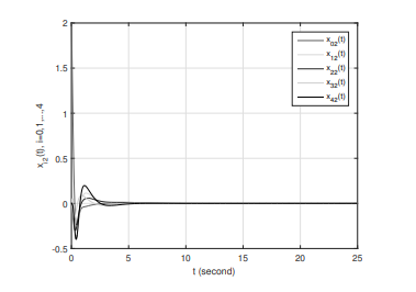
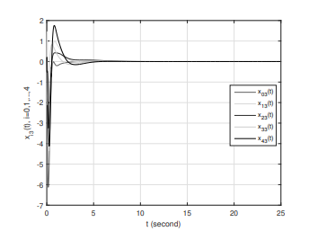
The control goal here is to design some pinning controllers to some designed agents such that the states of all the agents in $(5.33)$ to converge to a common target trajectory $s(t)$ in the sense of $\lim {t \rightarrow \infty}\left|x{i}(t)-s(t)\right|=0$, for all $i=1, \ldots, N$, with
$$
\dot{s}(t)=A s(t)+\beta s(t) B s(t),
$$
with arbitrarily given initial value $s\left(t_{0}\right) \in \mathbb{R}^{3}$. Motivated by the works in $[74,136$, $205,216]$, pinning CNS (5.33) by using some linear controllers $-\alpha c_{i}(t) H\left(x_{i}(t)-s(t)\right)$ to agent $i$ leads to
$$
\begin{aligned}
\dot{x}{i}(t)=& A x{i}(t)+\beta x_{i}(t) B x_{i}(t) \
&-\alpha \sum_{j=1}^{N} l_{i j}(t) H x_{j}(t)-\alpha c_{i}(t) H\left(x_{i}(t)-s(t)\right)
\end{aligned}
$$
where $c_{i}(t) \in{0,1}$ and $c_{i}(t)=1$ if the agent $i$ of $(5.33)$ is pinned at time $t$.
Let $e_{i}(t)=x_{i}(t)-s(t), i=1, \ldots, N$, it thus follows from (5.37) that
$$
\begin{aligned}
\dot{e}{i}(t)=& A e{i}(t)+\beta x_{i}(t) B x_{i}(t)-\beta s(t) B s(t) \
&-\alpha \sum_{j=1}^{N} l_{i j}(t) H e_{j}(t)-\alpha c_{i}(t) H e_{i}(t)
\end{aligned}
$$
cs代写|复杂网络代写complex network代考|Main results for directed fixed communication topology
In this subsection, consensus tracking of CNS (5.33) with target trajectory given in (5.36) under a fixed communication topology is studied. Without loss of generality, let $\mathcal{G}(\mathcal{A}(t))=\mathcal{G}(\mathcal{A})$ for all $t \geq 0$. And we label the target as agent 0 .
Assumption 5.2 There exists at least one directed spanning tree rooted at agent 0 (i.e., the target) in the augmented communication topology $\mathcal{G}(\widetilde{\mathcal{A}})$.
It is clearly that Assumption $5.2$ will hold if all the agents $1, \ldots, N$ are pinned, i.e., $c_{i}(t)=1$, for all $i=1, \ldots, N$ and $t \geq 0$. However, it is more interesting to study how to make Assumption $5.2$ hold if only a small fraction of the agents in $\mathcal{G}(\mathcal{A})$ could be selected and pinned. To do this, the following algorithm is proposed to determine at least how many and what kinds of agents should be pinned such that Assumption $5.2$ holds.
Algorithm 5.2 Find the strongly connected components of $\mathcal{G}(\mathcal{A})$ by employing the Tarjan’s algorithm [157]. Note that the time complexity of this operation is $O(N+E)$, where $N$ and $E$ are, respectively, the numbers of agents and links of $\mathcal{G}(\mathcal{A}) .$ Suppose that there are $\omega$ strongly connected components in $\mathcal{G}(\mathcal{A})$, labeled as $W_{1}, W_{2}, \ldots, W_{\omega}$. Set $m_{i}=0, i=1, \ldots, \omega$, and $h=1$. Then, execute the following steps
(1) Check whether there exists at least one agent $n_{k}$ belonging to $W_{h}$ which is reachable from an agent $n_{g}$ belonging to $W_{j}, j=1, \ldots, \omega, j \neq h$. If it holds, go to step (2); if it dose not hold, go to step (3).
(2) Check whether the following condition holds: $h<\omega$. If it holds, let $h=h+1$ and re-perform step (1); else stop.
(3) Arbitrarily selected one agent in $W_{h}$ and pinned, let $m_{h}=1$; Check whether the following condition holds: $h<\omega$. If it holds, let $h=h+1$ and re-perform step (1); else stop.
cs代写|复杂网络代写complex network代考|Main results for directed switching communication topologies
The underlying topology of the CNS considered in this subsection is modeled by directed switching graphs. Let $\overline{\mathcal{G}}=\left{\mathcal{G}\left(\mathcal{A}^{1}\right), \ldots, \mathcal{G}\left(\mathcal{A}^{\kappa}\right)\right}, \kappa \geq 2$, indicate the set of all possible directed communication topologies. Suppose that there exists an infinite sequence of uniformly bounded non-overlapping time intervals $\left[t_{k}, t_{k+1}\right), k \in \mathbb{N}$, with $t_{0}=0$, over which the interaction graph is fixed. The time sequence $t_{k}, k \in \mathbb{N}$ is then called the switching sequence, at which the interaction graph changes. Furthermore, introduce a switching signal $\sigma(t):[0,+\infty) \mapsto{1, \ldots, \kappa}$. Then, let $\mathcal{G}\left(\mathcal{A}^{\sigma(t)}\right)$ be the communication topology of the CNS at time $t$. Note that $\mathcal{G}\left(\mathcal{A}^{\sigma(t)}\right) \in \overline{\mathcal{G}}$, for all $t \geq 0$. The error dynamical system (5.39) can be rewritten as
$$
\begin{aligned}
\dot{e}{i}(t)=& A e{i}(t)+\beta x_{i}(t) B e_{i}(t)+\beta e_{i}(t) B s(t)-\alpha \sum_{j=1}^{N} l_{i j}^{\sigma(t)} H e_{j}(t) \
&-\alpha c_{i}(t) H e_{i}(t), i=1, \ldots, N,
\end{aligned}
$$
where $\mathcal{L}^{\sigma(t)}=\left[l_{i j}^{\sigma(t)}\right]{N \times N}$ is the Laplacian matrix of communication topology $\mathcal{G}\left(\mathcal{A}^{\sigma(t)}\right)$. Throughout this section, the time derivatives of functions $e{i}(t)$ and $x_{i}(t)$ at any switching instant represent its right derivative.
Assumption 5.3 There exists at least one directed spanning tree rooted at agent 0 (i.e., the target) in the augmented communication topology $\mathcal{G}\left(\widetilde{\mathcal{A}}^{\sigma(t)}\right)$.
Remark 5.10 Applying Algorithm $5.2$ to each possible communication topology $\mathcal{G}\left(\mathcal{A}^{i}\right), i=1, \ldots, \kappa$, one gets that Assumption $5.3$ will hold if the selected agents are pinned.
Similar to the last subsection, the Laplacian matrix of $\mathcal{G}\left(\tilde{\mathcal{A}}^{i}\right), i=1, \ldots, \kappa$, can be written as
$$
\begin{gathered}
\tilde{\mathcal{L}}^{i}=\left[\begin{array}{cc}
0 & \mathbf{0}{N}^{T} \ \mathbf{P}^{i} & \overline{\mathcal{L}}^{i} \end{array}\right], \ \overline{\mathcal{L}}^{i}=\left[\begin{array}{cccc} \sum{j \in N_{1}} a_{1 j}^{i} & -a_{12}^{i} & \cdots & -a_{1 N}^{i} \
-a_{21}^{i} & \sum_{j \in \mathcal{N}{2}} a{2 j}^{i} & \cdots & -a_{2 N}^{i} \
\vdots & \vdots & \ddots & \vdots \
-a_{N 1}^{i} & -a_{N 2}^{i} & \cdots & \sum_{j \in \mathcal{N}{N}} a{N j}^{i}
\end{array}\right],
\end{gathered}
$$
where $\mathbf{P}^{i}=-\left[a_{10}^{i}, \cdots, a_{N 0}^{i}\right]^{T}$. with $a_{j 0}^{i}=c_{j}^{i}, j=1, \ldots, N$. Under Assumption 5.3, it can be got from Lemma $2.15$ that there exists a sequence of positive definite diagonal matrices $\Phi^{i}=\operatorname{diag}\left{\phi_{1}^{i}, \ldots, \phi_{N}^{i}\right}$ such that $\left(\overline{\mathcal{L}}^{i}\right)^{T} \Phi^{i}+\Phi^{i} \overline{\mathcal{L}}^{i}>0$, where $\phi^{i}=$ $\left[\phi_{1}^{i}, \ldots, \phi_{N}^{i}\right]^{T}$ can be obtained by solving the matrix equation $\left(\overline{\mathcal{L}}^{i}\right)^{T} \phi^{i}=\mathbf{1}_{N}, i=$ $1, \ldots, \kappa$.
Based on the above analysis, one may get the following theorem which is the main result of this subsection.
复杂网络代写
cs代写|复杂网络代写complex network代考|Model formulation
考虑具有 Lorenz 型动力学的 CNS,由下式给出
X˙一世(吨)=一个X一世(吨)+bX一世(吨)乙X一世(吨)+一个∑j=1ñ一个一世j(吨)H(Xj(吨)−X一世(吨)),
在哪里
一个=[−(25C+10)(25C+10)0 (28−35C)(29C−1)0 00−(C+8)3],乙=[000 00−1 010],
b=[1,0,0],C∈[0,1]是一个参数,一个>0表示代理之间的耦合强度,一个(吨)=[一个一世j(吨)]ñ×ñ是通信拓扑在时间的邻接矩阵吨, 和H∈R3×3是正定内链接矩阵,一世=1,…,ñ. 请注意,系统 (5.33) 将成为耦合 Lorenz、Chen 和 Lü 系统,如果C=0,1, 和0.8, 分别。根据图的拉普拉斯矩阵的定义,从 (5.33) 可以得出
X˙一世(吨)=一个X一世(吨)+bX一世(吨)乙X一世(吨)−一个∑j=1ñl一世j(吨)HXj(吨),
在哪里大号(吨)=[l一世j(吨)]ñ×ñ是通信拓扑的拉普拉斯矩阵G(一个(吨)), 一世=1,…,ñ. 本节假设吨0=0.
这里的控制目标是为一些设计的代理设计一些固定控制器,使得所有代理的状态(5.33)收敛到一个共同的目标轨迹s(吨)在某种意义上林吨→∞|X一世(吨)−s(吨)|=0, 对全部一世=1,…,ñ, 和
s˙(吨)=一个s(吨)+bs(吨)乙s(吨),
具有任意给定的初始值s(吨0)∈R3. 受到作品的启发[74,136,205,216], 通过使用一些线性控制器固定 CNS (5.33)−一个C一世(吨)H(X一世(吨)−s(吨))代理一世导致
X˙一世(吨)=一个X一世(吨)+bX一世(吨)乙X一世(吨) −一个∑j=1ñl一世j(吨)HXj(吨)−一个C一世(吨)H(X一世(吨)−s(吨))
在哪里C一世(吨)∈0,1和C一世(吨)=1如果代理一世的(5.33)被固定在时间吨.
让和一世(吨)=X一世(吨)−s(吨),一世=1,…,ñ, 因此从 (5.37) 得出
和˙一世(吨)=一个和一世(吨)+bX一世(吨)乙X一世(吨)−bs(吨)乙s(吨) −一个∑j=1ñl一世j(吨)H和j(吨)−一个C一世(吨)H和一世(吨)
cs代写|复杂网络代写complex network代考|Main results for directed fixed communication topology
在本小节中,研究了在固定通信拓扑下使用(5.36)中给出的目标轨迹的 CNS(5.33)的一致性跟踪。不失一般性,让G(一个(吨))=G(一个)对所有人吨≥0. 我们将目标标记为代理 0 。
假设 5.2 增强通信拓扑中至少存在一棵以代理 0(即目标)为根的有向生成树G(一个~).
很明显,假设5.2如果所有代理都持有1,…,ñ被固定,即C一世(吨)=1, 对全部一世=1,…,ñ和吨≥0. 但是,更有趣的是研究如何进行假设5.2如果只有一小部分代理持有G(一个)可以选择和固定。为此,提出了以下算法来确定至少应该固定多少和什么样的代理,这样假设5.2持有。
算法 5.2 求强连通分量G(一个)通过采用 Tarjan 算法 [157]。注意这个操作的时间复杂度是○(ñ+和), 在哪里ñ和和分别是代理的数量和链接的数量G(一个).假设有ω强连通分量G(一个),标记为在1,在2,…,在ω. 放米一世=0,一世=1,…,ω, 和H=1. 然后,执行以下步骤
(1) 检查是否存在至少一个代理nķ属于在H可以从代理访问nG属于在j,j=1,…,ω,j≠H. 如果成立,则进行步骤(2);如果不成立,转至步骤(3)。
(2) 检查下列条件是否成立:H<ω. 如果它成立,让H=H+1并重新执行步骤(1);否则停止。
(3) 任意选择一名代理人在H并固定,让米H=1; 检查以下条件是否成立:H<ω. 如果它成立,让H=H+1并重新执行步骤(1);否则停止。
cs代写|复杂网络代写complex network代考|Main results for directed switching communication topologies
本小节中考虑的 CNS 的底层拓扑结构由有向开关图建模。让\overline{\mathcal{G}}=\left{\mathcal{G}\left(\mathcal{A}^{1}\right), \ldots, \mathcal{G}\left(\mathcal{A} ^{\kappa}\right)\right}, \kappa \geq 2\overline{\mathcal{G}}=\left{\mathcal{G}\left(\mathcal{A}^{1}\right), \ldots, \mathcal{G}\left(\mathcal{A} ^{\kappa}\right)\right}, \kappa \geq 2,表示所有可能的有向通信拓扑的集合。假设存在无限的均匀有界非重叠时间间隔序列[吨ķ,吨ķ+1),ķ∈ñ, 和吨0=0,其上的交互图是固定的。时间顺序吨ķ,ķ∈ñ然后称为切换序列,在该切换序列处交互图发生变化。此外,引入一个开关信号σ(吨):[0,+∞)↦1,…,ķ. 那么,让G(一个σ(吨))是当时 CNS 的通信拓扑吨. 注意G(一个σ(吨))∈G¯, 对全部吨≥0. 误差动态系统(5.39)可以重写为
和˙一世(吨)=一个和一世(吨)+bX一世(吨)乙和一世(吨)+b和一世(吨)乙s(吨)−一个∑j=1ñl一世jσ(吨)H和j(吨) −一个C一世(吨)H和一世(吨),一世=1,…,ñ,
在哪里大号σ(吨)=[l一世jσ(吨)]ñ×ñ是通信拓扑的拉普拉斯矩阵G(一个σ(吨)). 在本节中,函数的时间导数和一世(吨)和X一世(吨)在任何切换时刻代表它的右导数。
假设 5.3 增强通信拓扑中至少存在一棵以代理 0(即目标)为根的有向生成树G(一个~σ(吨)).
备注 5.10 应用算法5.2到每个可能的通信拓扑G(一个一世),一世=1,…,ķ,一个人得到那个假设5.3如果选定的代理被固定,将保持。
与上一小节类似,拉普拉斯矩阵G(一个~一世),一世=1,…,ķ, 可以写成
大号~一世=[00ñ吨 磷一世大号¯一世], 大号¯一世=[∑j∈ñ1一个1j一世−一个12一世⋯−一个1ñ一世 −一个21一世∑j∈ñ2一个2j一世⋯−一个2ñ一世 ⋮⋮⋱⋮ −一个ñ1一世−一个ñ2一世⋯∑j∈ññ一个ñj一世],
在哪里磷一世=−[一个10一世,⋯,一个ñ0一世]吨. 和一个j0一世=Cj一世,j=1,…,ñ. 在假设 5.3 下,可以从引理得到2.15存在一系列正定对角矩阵\Phi^{i}=\operatorname{diag}\left{\phi_{1}^{i}, \ldots, \phi_{N}^{i}\right}\Phi^{i}=\operatorname{diag}\left{\phi_{1}^{i}, \ldots, \phi_{N}^{i}\right}这样(大号¯一世)吨披一世+披一世大号¯一世>0, 在哪里φ一世= [φ1一世,…,φñ一世]吨可以通过求解矩阵方程得到(大号¯一世)吨φ一世=1ñ,一世= 1,…,ķ.
基于以上分析,可以得到以下定理,这是本小节的主要结果。

统计代写请认准statistics-lab™. statistics-lab™为您的留学生涯保驾护航。
金融工程代写
金融工程是使用数学技术来解决金融问题。金融工程使用计算机科学、统计学、经济学和应用数学领域的工具和知识来解决当前的金融问题,以及设计新的和创新的金融产品。
非参数统计代写
非参数统计指的是一种统计方法,其中不假设数据来自于由少数参数决定的规定模型;这种模型的例子包括正态分布模型和线性回归模型。
广义线性模型代考
广义线性模型(GLM)归属统计学领域,是一种应用灵活的线性回归模型。该模型允许因变量的偏差分布有除了正态分布之外的其它分布。
术语 广义线性模型(GLM)通常是指给定连续和/或分类预测因素的连续响应变量的常规线性回归模型。它包括多元线性回归,以及方差分析和方差分析(仅含固定效应)。
有限元方法代写
有限元方法(FEM)是一种流行的方法,用于数值解决工程和数学建模中出现的微分方程。典型的问题领域包括结构分析、传热、流体流动、质量运输和电磁势等传统领域。
有限元是一种通用的数值方法,用于解决两个或三个空间变量的偏微分方程(即一些边界值问题)。为了解决一个问题,有限元将一个大系统细分为更小、更简单的部分,称为有限元。这是通过在空间维度上的特定空间离散化来实现的,它是通过构建对象的网格来实现的:用于求解的数值域,它有有限数量的点。边界值问题的有限元方法表述最终导致一个代数方程组。该方法在域上对未知函数进行逼近。[1] 然后将模拟这些有限元的简单方程组合成一个更大的方程系统,以模拟整个问题。然后,有限元通过变化微积分使相关的误差函数最小化来逼近一个解决方案。
tatistics-lab作为专业的留学生服务机构,多年来已为美国、英国、加拿大、澳洲等留学热门地的学生提供专业的学术服务,包括但不限于Essay代写,Assignment代写,Dissertation代写,Report代写,小组作业代写,Proposal代写,Paper代写,Presentation代写,计算机作业代写,论文修改和润色,网课代做,exam代考等等。写作范围涵盖高中,本科,研究生等海外留学全阶段,辐射金融,经济学,会计学,审计学,管理学等全球99%专业科目。写作团队既有专业英语母语作者,也有海外名校硕博留学生,每位写作老师都拥有过硬的语言能力,专业的学科背景和学术写作经验。我们承诺100%原创,100%专业,100%准时,100%满意。
随机分析代写
随机微积分是数学的一个分支,对随机过程进行操作。它允许为随机过程的积分定义一个关于随机过程的一致的积分理论。这个领域是由日本数学家伊藤清在第二次世界大战期间创建并开始的。
时间序列分析代写
随机过程,是依赖于参数的一组随机变量的全体,参数通常是时间。 随机变量是随机现象的数量表现,其时间序列是一组按照时间发生先后顺序进行排列的数据点序列。通常一组时间序列的时间间隔为一恒定值(如1秒,5分钟,12小时,7天,1年),因此时间序列可以作为离散时间数据进行分析处理。研究时间序列数据的意义在于现实中,往往需要研究某个事物其随时间发展变化的规律。这就需要通过研究该事物过去发展的历史记录,以得到其自身发展的规律。
回归分析代写
多元回归分析渐进(Multiple Regression Analysis Asymptotics)属于计量经济学领域,主要是一种数学上的统计分析方法,可以分析复杂情况下各影响因素的数学关系,在自然科学、社会和经济学等多个领域内应用广泛。
MATLAB代写
MATLAB 是一种用于技术计算的高性能语言。它将计算、可视化和编程集成在一个易于使用的环境中,其中问题和解决方案以熟悉的数学符号表示。典型用途包括:数学和计算算法开发建模、仿真和原型制作数据分析、探索和可视化科学和工程图形应用程序开发,包括图形用户界面构建MATLAB 是一个交互式系统,其基本数据元素是一个不需要维度的数组。这使您可以解决许多技术计算问题,尤其是那些具有矩阵和向量公式的问题,而只需用 C 或 Fortran 等标量非交互式语言编写程序所需的时间的一小部分。MATLAB 名称代表矩阵实验室。MATLAB 最初的编写目的是提供对由 LINPACK 和 EISPACK 项目开发的矩阵软件的轻松访问,这两个项目共同代表了矩阵计算软件的最新技术。MATLAB 经过多年的发展,得到了许多用户的投入。在大学环境中,它是数学、工程和科学入门和高级课程的标准教学工具。在工业领域,MATLAB 是高效研究、开发和分析的首选工具。MATLAB 具有一系列称为工具箱的特定于应用程序的解决方案。对于大多数 MATLAB 用户来说非常重要,工具箱允许您学习和应用专业技术。工具箱是 MATLAB 函数(M 文件)的综合集合,可扩展 MATLAB 环境以解决特定类别的问题。可用工具箱的领域包括信号处理、控制系统、神经网络、模糊逻辑、小波、仿真等。