如果你也在 怎样代写机器学习machine learning这个学科遇到相关的难题,请随时右上角联系我们的24/7代写客服。
机器学习(ML)是人工智能(AI)的一种类型,它允许软件应用程序在预测结果时变得更加准确,而无需明确编程。机器学习算法使用历史数据作为输入来预测新的输出值。
statistics-lab™ 为您的留学生涯保驾护航 在代写机器学习machine learning方面已经树立了自己的口碑, 保证靠谱, 高质且原创的统计Statistics代写服务。我们的专家在代写机器学习machine learning代写方面经验极为丰富,各种代写机器学习machine learning相关的作业也就用不着说。
我们提供的机器学习machine learning及其相关学科的代写,服务范围广, 其中包括但不限于:
- Statistical Inference 统计推断
- Statistical Computing 统计计算
- Advanced Probability Theory 高等概率论
- Advanced Mathematical Statistics 高等数理统计学
- (Generalized) Linear Models 广义线性模型
- Statistical Machine Learning 统计机器学习
- Longitudinal Data Analysis 纵向数据分析
- Foundations of Data Science 数据科学基础
cs代写|机器学习代写machine learning代考|Soft margin classifier
Thus far we have only discussed the linear separable case, but how about the case when there are overlapping classes? It is possible to extend the optimization problem by allowing some data points to be in the margin while penalizing these points somewhat. We therefore include some slag variables $\xi_{i}$ that reduce the effective margin for each data point, but we add a penalty term to the optimization that penalizes if the sum of these slag variables are large,
$$
\min {\mathbf{w}, b} \frac{1}{2}|\mathbf{w}|^{2}+C \sum{i} \xi_{i}
$$
subject to the constraints
$$
\begin{aligned}
y^{(i)}\left(\mathbf{w}^{T} \mathbf{x}+b\right) & \geq 1-\xi_{i} \
\xi_{i} & \geq 0
\end{aligned}
$$
The constant $C$ is a free parameter in this algorithm. Making this constant large means allowing fewer points to be in the margin. This parameter must be tuned and it is advisable at least to try to vary this parameter in order to verify that the results do not dramatically depend on an initial choice.
cs代写|机器学习代写machine learning代考|Non-linear support vector machines
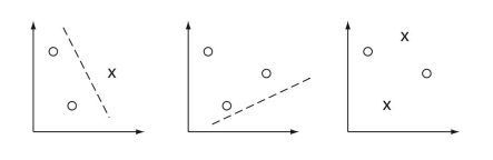
We have treated the case of overlapping classes while assuming that the best we can do is a linear separation. However, what if the underlying problem is separable with a function that might be more complex? An example is shown in Fig. 3.10. Nonlinear separation and regression models are of course much more common in machine learning, and we will now look into the non-linear generalization of the SVM.
Let us illustrate the basic idea with an example in two-dimensions. A linear function with two attributes that span the 2-dimensional feature space is given by
$$
y=w_{0}+w_{1} x_{1}+w_{2} x_{2}=\mathbf{w}^{T} \mathbf{x},
$$
with
$$
\mathbf{x}=\left(\begin{array}{c}
1 \
x_{1} \
x_{2}
\end{array}\right)
$$
and weight vector
$$
\mathbf{w}^{T}=\left(w_{0}, w_{1}, w_{2}\right) .
$$
Let us say that we cannot separate the data with this linear function but that we could separate it with a polynomial that include second-order terms like
$$
y=\tilde{w}{0}+\tilde{w}{1} x_{1}+\tilde{w}{2} x{2}+\tilde{w}{3} x{1} x_{2}+\tilde{w}{4} x{1}^{2}+\tilde{w}{5} x{2}^{2}=\tilde{\mathbf{w}} \phi(\mathbf{x}) .
$$
We can view the second equation as a linear separation on a feature vector
$$
\mathbf{x} \rightarrow \phi(\mathbf{x})=\left(\begin{array}{c}
1 \
x_{1} \
x_{2} \
x_{1} x_{2} \
x_{1}^{2} \
x_{2}^{2}
\end{array}\right) .
$$
This can be seen as mapping the attribute space $\left(1, x_{1}, x_{2}\right)$ to a higher-dimensional space with the mapping function $\phi(\mathbf{x})$. We call this mapping a feature map. The separating hyperplane is then linear in this higher-dimensional space. Thus, we can use the above linear maximum margin classification method in non-linear cases if we replace all occurrences of the attribute vector $x$ with the mapped feature vector $\phi(\mathbf{x})$.
There are only three problems remaining. One is that we don’t know what the mapping function should be. The somewhat ad-hoc solution to this problem will be that we try out some functions and see which one works best. We will discuss this further later in this chapter. The second problem is that we have the problem of overfitting
as we might use too many feature dimensions and corresponding free parameters $w_{i}$. In the next section, we provide a glimpse of an argument why SVMs might address this problem. The third problem is that with an increased number of dimensions the evaluation of the equations becomes more computational intensive. However, there is a useful trick to alleviate the last problem in the case when the calculations always contain only dot products between feature vectors. An example of this is the solution of the minimization problem of the dual problem in the earlier discussions of the linear SVM. The function to be minimized in this formulation, Egn $3.26$ with the feature maps, only depends on the dot products between a vector $\mathbf{x}^{(i)}$ of one example and another example $\mathbf{x}^{(j)}$. Also, when predicting the class for a new input vector $\mathbf{x}$ from Egn $3.24$ when adding the feature maps, we only need the resulting values for the dot products $\phi\left(\mathbf{x}^{(i)}\right)^{T} \phi(\mathbf{x})$. We now discuss that such dot products can sometimes be represented with functions called kernel functions,
$$
K(\mathbf{x}, \mathbf{z})=\phi(\mathbf{x})^{T} \phi(\mathbf{z})
$$
Instead of actually specifying a feature map, which is often a guess to start with, we could actually specify a kernel function. For example, let us consider a quadratic kernel function between two vectors $\mathbf{x}$ and $\mathbf{z}$,
$$
K(\mathbf{x}, \mathbf{z})=\left(\mathbf{x}^{T} \mathbf{z}+1\right)^{2}
$$
cs代写|机器学习代写machine learning代考|Statistical learning theory and VC dimension
SVMs are good and practical classification algorithms for several reasons. In particular, they are formulated as a convex optimization problem that has many good theoretical properties and that can be solved with quadratic programming. They are formulated to
take advantage of the kernel trick, they have a compact representation of the decision hyperplane with support vectors, and turn out to be fairly robust with respect to the hyper parameters. However, in order to act as a good learner, they need to moderate the overfitting problem discussed earlier. A great theoretical contributions of Vapnik and colleagues was the embedding of supervised learning into statistical learning theory and to derive some bounds that make statements on the average ability to learn form data. We briefly outline here the ideas and state some of the results without too much details, and we discuss this issue here entirely in the context of binary classification. However, similar observations can be made in the case of multiclass classification and regression. This section uses language from probability theory that we only introduce in more detail later. Therefore, this section might be best viewed at a later stage. Again, the main reason in placing this section is to outline the deeper reasoning for specific models.
As can’t be stressed enough, our objective in supervised machine learning is to find a good model which minimizes the generalization error. To state this differently by using nomenclature common in these discussions, we call the error function here the risk function $R$; in particular, the expected risk. In the case of binary classification, this is the probability of missclassification,
$$
R(h)=P(h(x) \neq y)
$$
Of course, we generally do not know this density function. We assume here that the samples are iid (independent and identical distributed) data, and we can then estimate what is called the empirical risk with the help of the test data,
$$
\hat{R}(h)=\frac{1}{m} \sum_{i=1}^{m} \mathbb{1}\left(h\left(\mathbf{x}^{(i)} ; \theta\right)=y^{(i)}\right)
$$
机器学习代写
cs代写|机器学习代写machine learning代考|Soft margin classifier
到目前为止,我们只讨论了线性可分的情况,但是有重叠类的情况呢?可以通过允许一些数据点在边缘同时对这些点进行一些惩罚来扩展优化问题。因此,我们包括一些渣变量X一世这会降低每个数据点的有效边距,但我们会在优化中添加一个惩罚项,如果这些渣变量的总和很大,则会受到惩罚,
分钟在,b12|在|2+C∑一世X一世
受约束
是(一世)(在吨X+b)≥1−X一世 X一世≥0
常数C是该算法中的自由参数。使这个常数变大意味着允许更少的点在边缘。必须调整此参数,并且建议至少尝试更改此参数以验证结果不会显着依赖于初始选择。
cs代写|机器学习代写machine learning代考|Non-linear support vector machines
我们已经处理了重叠类的情况,同时假设我们能做的最好的是线性分离。但是,如果潜在问题可以与可能更复杂的函数分开怎么办?示例如图 3.10 所示。非线性分离和回归模型当然在机器学习中更为常见,我们现在将研究 SVM 的非线性泛化。
让我们用一个二维的例子来说明这个基本思想。具有跨越二维特征空间的两个属性的线性函数由下式给出
是=在0+在1X1+在2X2=在吨X,
和
X=(1 X1 X2)
和权重向量
在吨=(在0,在1,在2).
假设我们不能用这个线性函数分离数据,但我们可以用一个包含二阶项的多项式来分离它,比如
是=在~0+在~1X1+在~2X2+在~3X1X2+在~4X12+在~5X22=在~φ(X).
我们可以将第二个方程视为特征向量上的线性分离
X→φ(X)=(1 X1 X2 X1X2 X12 X22).
这可以看作是映射属性空间(1,X1,X2)到具有映射函数的高维空间φ(X). 我们称这种映射为特征图。分离的超平面在这个高维空间中是线性的。因此,如果我们替换所有出现的属性向量,我们可以在非线性情况下使用上述线性最大边距分类方法X与映射的特征向量φ(X).
只剩下三个问题了。一是我们不知道映射函数应该是什么。这个问题的某种临时解决方案是我们尝试一些功能,看看哪一个效果最好。我们将在本章后面进一步讨论这个问题。第二个问题是我们有过拟合的问题
因为我们可能会使用太多的特征维度和相应的自由参数在一世. 在下一节中,我们将简要介绍为什么 SVM 可以解决这个问题。第三个问题是,随着维数的增加,方程的评估变得更加计算密集。然而,当计算总是只包含特征向量之间的点积时,有一个有用的技巧可以缓解最后一个问题。这方面的一个例子是前面讨论的线性 SVM 中对偶问题的最小化问题的解决方案。在这个公式中要最小化的函数,Egn3.26使用特征图,仅取决于向量之间的点积X(一世)一个例子和另一个例子X(j). 此外,在预测新输入向量的类别时X来自 Egn3.24添加特征图时,我们只需要点积的结果值φ(X(一世))吨φ(X). 我们现在讨论这种点积有时可以用称为核函数的函数来表示,
ķ(X,和)=φ(X)吨φ(和)
我们实际上可以指定一个核函数,而不是实际指定一个特征图,这通常是一个猜测。例如,让我们考虑两个向量之间的二次核函数X和和,
ķ(X,和)=(X吨和+1)2
cs代写|机器学习代写machine learning代考|Statistical learning theory and VC dimension
支持向量机是很好且实用的分类算法,原因有几个。特别是,它们被表述为一个凸优化问题,该问题具有许多良好的理论性质并且可以通过二次规划来解决。它们被制定为
利用内核技巧,它们具有带有支持向量的决策超平面的紧凑表示,并且在超参数方面相当稳健。然而,为了成为一个好的学习者,他们需要缓和前面讨论的过度拟合问题。Vapnik 及其同事的一个重要理论贡献是将监督学习嵌入到统计学习理论中,并得出了一些关于学习表格数据的平均能力的陈述。我们在这里简要概述了这些想法并在没有太多细节的情况下陈述了一些结果,并且我们在这里完全在二进制分类的背景下讨论了这个问题。但是,在多类分类和回归的情况下可以进行类似的观察。本节使用概率论中的语言,稍后我们将更详细地介绍。因此,最好在稍后阶段查看此部分。同样,放置本节的主要原因是概述特定模型的更深层次的推理。
怎么强调都不为过,我们在监督机器学习中的目标是找到一个好的模型来最小化泛化误差。为了通过使用这些讨论中常见的命名法来不同地说明这一点,我们将这里的误差函数称为风险函数R; 特别是预期风险。在二分类的情况下,这是错误分类的概率,
R(H)=磷(H(X)≠是)
当然,我们一般不知道这个密度函数。我们在这里假设样本是 iid(独立同分布)数据,然后我们可以借助测试数据估计所谓的经验风险,
R^(H)=1米∑一世=1米1(H(X(一世);θ)=是(一世))

统计代写请认准statistics-lab™. statistics-lab™为您的留学生涯保驾护航。
金融工程代写
金融工程是使用数学技术来解决金融问题。金融工程使用计算机科学、统计学、经济学和应用数学领域的工具和知识来解决当前的金融问题,以及设计新的和创新的金融产品。
非参数统计代写
非参数统计指的是一种统计方法,其中不假设数据来自于由少数参数决定的规定模型;这种模型的例子包括正态分布模型和线性回归模型。
广义线性模型代考
广义线性模型(GLM)归属统计学领域,是一种应用灵活的线性回归模型。该模型允许因变量的偏差分布有除了正态分布之外的其它分布。
术语 广义线性模型(GLM)通常是指给定连续和/或分类预测因素的连续响应变量的常规线性回归模型。它包括多元线性回归,以及方差分析和方差分析(仅含固定效应)。
有限元方法代写
有限元方法(FEM)是一种流行的方法,用于数值解决工程和数学建模中出现的微分方程。典型的问题领域包括结构分析、传热、流体流动、质量运输和电磁势等传统领域。
有限元是一种通用的数值方法,用于解决两个或三个空间变量的偏微分方程(即一些边界值问题)。为了解决一个问题,有限元将一个大系统细分为更小、更简单的部分,称为有限元。这是通过在空间维度上的特定空间离散化来实现的,它是通过构建对象的网格来实现的:用于求解的数值域,它有有限数量的点。边界值问题的有限元方法表述最终导致一个代数方程组。该方法在域上对未知函数进行逼近。[1] 然后将模拟这些有限元的简单方程组合成一个更大的方程系统,以模拟整个问题。然后,有限元通过变化微积分使相关的误差函数最小化来逼近一个解决方案。
tatistics-lab作为专业的留学生服务机构,多年来已为美国、英国、加拿大、澳洲等留学热门地的学生提供专业的学术服务,包括但不限于Essay代写,Assignment代写,Dissertation代写,Report代写,小组作业代写,Proposal代写,Paper代写,Presentation代写,计算机作业代写,论文修改和润色,网课代做,exam代考等等。写作范围涵盖高中,本科,研究生等海外留学全阶段,辐射金融,经济学,会计学,审计学,管理学等全球99%专业科目。写作团队既有专业英语母语作者,也有海外名校硕博留学生,每位写作老师都拥有过硬的语言能力,专业的学科背景和学术写作经验。我们承诺100%原创,100%专业,100%准时,100%满意。
随机分析代写
随机微积分是数学的一个分支,对随机过程进行操作。它允许为随机过程的积分定义一个关于随机过程的一致的积分理论。这个领域是由日本数学家伊藤清在第二次世界大战期间创建并开始的。
时间序列分析代写
随机过程,是依赖于参数的一组随机变量的全体,参数通常是时间。 随机变量是随机现象的数量表现,其时间序列是一组按照时间发生先后顺序进行排列的数据点序列。通常一组时间序列的时间间隔为一恒定值(如1秒,5分钟,12小时,7天,1年),因此时间序列可以作为离散时间数据进行分析处理。研究时间序列数据的意义在于现实中,往往需要研究某个事物其随时间发展变化的规律。这就需要通过研究该事物过去发展的历史记录,以得到其自身发展的规律。
回归分析代写
多元回归分析渐进(Multiple Regression Analysis Asymptotics)属于计量经济学领域,主要是一种数学上的统计分析方法,可以分析复杂情况下各影响因素的数学关系,在自然科学、社会和经济学等多个领域内应用广泛。
MATLAB代写
MATLAB 是一种用于技术计算的高性能语言。它将计算、可视化和编程集成在一个易于使用的环境中,其中问题和解决方案以熟悉的数学符号表示。典型用途包括:数学和计算算法开发建模、仿真和原型制作数据分析、探索和可视化科学和工程图形应用程序开发,包括图形用户界面构建MATLAB 是一个交互式系统,其基本数据元素是一个不需要维度的数组。这使您可以解决许多技术计算问题,尤其是那些具有矩阵和向量公式的问题,而只需用 C 或 Fortran 等标量非交互式语言编写程序所需的时间的一小部分。MATLAB 名称代表矩阵实验室。MATLAB 最初的编写目的是提供对由 LINPACK 和 EISPACK 项目开发的矩阵软件的轻松访问,这两个项目共同代表了矩阵计算软件的最新技术。MATLAB 经过多年的发展,得到了许多用户的投入。在大学环境中,它是数学、工程和科学入门和高级课程的标准教学工具。在工业领域,MATLAB 是高效研究、开发和分析的首选工具。MATLAB 具有一系列称为工具箱的特定于应用程序的解决方案。对于大多数 MATLAB 用户来说非常重要,工具箱允许您学习和应用专业技术。工具箱是 MATLAB 函数(M 文件)的综合集合,可扩展 MATLAB 环境以解决特定类别的问题。可用工具箱的领域包括信号处理、控制系统、神经网络、模糊逻辑、小波、仿真等。