如果你也在 怎样代写有限元方法finite differences method 这个学科遇到相关的难题,请随时右上角联系我们的24/7代写客服。有限元方法finite differences method领域中所有的物理系统都可以用边界/初值问题来表示。在这本书中,我们主要集中在解决一维和二维线性弹性和传热问题。将这些解决方案技术扩展到三维分析是直接的,因此为了保持表示的清晰性并避免重复,这里不进行讨论。
有限元方法finite differences method提供了一种系统的方法来推导简单子区域的近似函数,通过这些近似函数可以表示几何上复杂的区域。在有限元法中,近似函数是分段多项式(即只在子区域上定义的多项式,称为单元)。
statistics-lab™ 为您的留学生涯保驾护航 在代写有限元方法Finite Element Method方面已经树立了自己的口碑, 保证靠谱, 高质且原创的统计Statistics代写服务。我们的专家在代写有限元方法Finite Element Method代写方面经验极为丰富,各种代写有限元方法Finite Element Method相关的作业也就用不着说。

数学代写|有限元方法代写Finite Element Method代考|Euler-Bernoulli beam theory
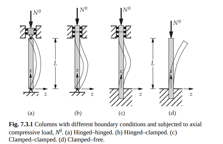
The study of buckling (also called stability) of beam-columns also leads to an eigenvalue problem. For example, equation governing the onset of buckling of a column subjected to an axial compressive force $N^0$ (see Fig. 7.3.1) according to the Euler-Bernoulli beam theory is (see Reddy [1,2])
$$
\frac{d^2}{d x^2}\left(E I \frac{d^2 W}{d x^2}\right)+N^0 \frac{d^2 W}{d x^2}=0
$$
where $W(x)$ is the lateral deflection at the onset of buckling. Equation (7.3.31) describes an eigenvalue problem with $\lambda=N^0$. The smallest value of $N^0$ is called the critical buckling load.
7.3.4.2 Timoshenko beam theory
For the Timoshenko beam theory, the equations governing buckling of beams are given by
$$
\begin{aligned}
&- \frac{d}{d x}\left[G A K_s\left(\frac{d W}{d x}+S\right)\right]+N^0 \frac{d^2 W}{d x^2}=0 \
&-\frac{d}{d x}\left(E I \frac{d S}{d x}\right)+G A K_s\left(\frac{d W}{d x}+S\right)=0
\end{aligned}
$$
Here $W(x)$ and $S(x)$ denote the transverse deflection and rotation,respectively, at the onset of buckling. Equations (7.3.32a) and (7.3.32b) together define an eigenvalue problem of finding the buckling load $N^0$ (eigenvalue) and the associated mode shape defined by $W(x)$ and $S(x)$ (eigenvector).
This completes the descriptions of the types of eigenvalue problems that will be treated in this chapter. The task of determining natural frequencies and mode shapes of a structure undergoing free (or natural) vibration is termed modal analysis. In addition, we also study buckling of beam-columns. In the following sections, we develop weak forms and finite element models of the eigenvalue problems described here. Numerical examples will be presented to illustrate the procedure of determining eigenvalues and eigenvectors, although this exercise may be familiar to the readers from other courses (e.g., a course on vibrations).
数学代写|有限元方法代写Finite Element Method代考|Finite Element Models
In this section, we develop finite element models of eigenvalue problems described by differential equations of heat transfer, bars, and beams. In view of the close similarity between the differential equations governing eigenvalue and boundary value problems, the steps involved in the construction of their finite element models are entirely analogous. The eigenvalue problems described by differential equations are reduced to algebraic eigenvalue problems by means of finite element approximations. The methods of solution of algebraic eigenvalue problems are then used to solve for the eigenvalues $\lambda$ and eigenvectors.
We note that a continuous system has an infinite number of eigenvalues while a discrete system has only a finite number of eigenvalues. The number of eigenvalues is equal to the number of unconstrained primary degrees of freedom in the mesh. The number of eigenvalues will increase with a mesh refinement, and the newly added eigenvalues will be larger in magnitude.
7.3.5.1 Heat transfer and bar-like problems (second-order equations)
Governing equation. The eigenvalue problem associated with onedimensional heat flow and straight bars both share the same type of governing equation:
$$
-\frac{d}{d x}\left(a \frac{d U}{d x}\right)+c_0 U-c \lambda U=0, \quad 0<x<L
$$
Here $a, c_0$ and $c$ are known parameters (data) that depend on the physical problem, $\lambda$ is the eigenvalue, and $U$ is the eigenfunction. Special cases of Eq. (7.3.33) are given below.
Heat transfer: $a=k A, c_0=P \beta, c=\rho c_v A$
Bars: $a=E A, c_0=0, c=c_2=\rho A$
Weak form. In view of the discussion of Chapters 3 and 4 , the weak form of Eq. (7.3.33) over $\Omega^e=\left(x_a^e, x_b^e\right)$ can be readily obtained as
$$
0=\int_{x_a^e}^{x_b^{\prime}}\left(a \frac{d w_i}{d x} \frac{d U_h}{d x}+c_0 w_i U_h-\lambda c w_i U_h\right) d x-Q_1^e w_i\left(x_a^e\right)-Q_n^e w_i\left(x_b^e\right)
$$
where $U_h$ is an approximation of $U, w_i$ is the ith weight function (which will be replaced with $\psi_i^e$ in deriving the finite element model), and $Q_1^e$ and $Q_n^e$ are the secondary variables at the first and last nodes, respectively, of a finite element with $n$ nodes (for eigenvalue problems, we take $Q_i^e=0$ for $1<i<n$ ):
$$
Q_1^e=-\left[a \frac{d U_h}{d x}\right]{x_a^e}, \quad Q_n^e=\left[a \frac{d U_h}{d x}\right]{x_b^e}
$$
有限元方法代考
数学代写|有限元方法代写Finite Element Method代考|Euler-Bernoulli beam theory
研究梁柱的屈曲(也称为稳定性)也会导致一个特征值问题。例如,根据欧拉-伯努利梁理论,柱在轴向压缩力$N^0$(见图7.3.1)作用下的屈曲起始方程为(见Reddy[1,2])。
$$
\frac{d^2}{d x^2}\left(E I \frac{d^2 W}{d x^2}\right)+N^0 \frac{d^2 W}{d x^2}=0
$$
其中$W(x)$为屈曲开始时的侧向挠度。式(7.3.31)描述了一个带有$\lambda=N^0$的特征值问题。$N^0$的最小值称为临界屈曲载荷。
7.3.4.2 Timoshenko梁理论
对于Timoshenko梁理论,控制梁屈曲的方程由
$$
\begin{aligned}
&- \frac{d}{d x}\left[G A K_s\left(\frac{d W}{d x}+S\right)\right]+N^0 \frac{d^2 W}{d x^2}=0 \
&-\frac{d}{d x}\left(E I \frac{d S}{d x}\right)+G A K_s\left(\frac{d W}{d x}+S\right)=0
\end{aligned}
$$
这里$W(x)$和$S(x)$分别表示屈曲开始时的横向挠度和旋转。式(7.3.32a)和式(7.3.32b)共同定义了一个求屈曲载荷$N^0$ (eigenvalue)和相关模态振型$W(x)$和$S(x)$ (eigenvector)的特征值问题。
这就完成了本章将要讨论的特征值问题类型的描述。确定经受自由(或固有)振动的结构的固有频率和模态振型的任务称为模态分析。此外,我们还研究了梁柱的屈曲。在接下来的章节中,我们将开发这里描述的特征值问题的弱形式和有限元模型。本文将给出数值例子来说明确定特征值和特征向量的过程,尽管读者可能对其他课程(例如振动课程)的练习很熟悉。
数学代写|有限元方法代写Finite Element Method代考|Finite Element Models
在本节中,我们开发了由传热、杆和梁的微分方程描述的特征值问题的有限元模型。由于特征值问题和边值问题的微分方程非常相似,它们的有限元模型的建立步骤是完全相似的。利用有限元逼近的方法,将微分方程所描述的特征值问题化为代数特征值问题。然后用代数特征值问题的解法求解特征值$\lambda$和特征向量。
我们注意到一个连续系统有无限个特征值,而一个离散系统只有有限个特征值。特征值的个数等于网格中无约束的初级自由度的个数。随着网格的细化,特征值的数量会增加,新增加的特征值的大小也会增大。
7.3.5.1传热和棒状问题(二阶方程)
控制方程。一维热流和直杆的特征值问题具有相同类型的控制方程:
$$
-\frac{d}{d x}\left(a \frac{d U}{d x}\right)+c_0 U-c \lambda U=0, \quad 0<x<L
$$
这里$a, c_0$和$c$是依赖于物理问题的已知参数(数据),$\lambda$是特征值,$U$是特征函数。(7.3.33)式的特殊情况如下。
传热:$a=k A, c_0=P \beta, c=\rho c_v A$
酒吧:$a=E A, c_0=0, c=c_2=\rho A$
弱形式。考虑到第3章和第4章的讨论,(7.3.33)式除以$\Omega^e=\left(x_a^e, x_b^e\right)$的弱形式可以很容易地得到
$$
0=\int_{x_a^e}^{x_b^{\prime}}\left(a \frac{d w_i}{d x} \frac{d U_h}{d x}+c_0 w_i U_h-\lambda c w_i U_h\right) d x-Q_1^e w_i\left(x_a^e\right)-Q_n^e w_i\left(x_b^e\right)
$$
其中$U_h$是近似的$U, w_i$是第i个权重函数(在推导有限元模型时将用$\psi_i^e$代替),$Q_1^e$和$Q_n^e$分别是具有$n$节点的有限元的第一个和最后一个节点上的次要变量(对于特征值问题,我们将$Q_i^e=0$作为$1<i<n$):
$$
Q_1^e=-\left[a \frac{d U_h}{d x}\right]{x_a^e}, \quad Q_n^e=\left[a \frac{d U_h}{d x}\right]{x_b^e}
$$

统计代写请认准statistics-lab™. statistics-lab™为您的留学生涯保驾护航。
金融工程代写
金融工程是使用数学技术来解决金融问题。金融工程使用计算机科学、统计学、经济学和应用数学领域的工具和知识来解决当前的金融问题,以及设计新的和创新的金融产品。
非参数统计代写
非参数统计指的是一种统计方法,其中不假设数据来自于由少数参数决定的规定模型;这种模型的例子包括正态分布模型和线性回归模型。
广义线性模型代考
广义线性模型(GLM)归属统计学领域,是一种应用灵活的线性回归模型。该模型允许因变量的偏差分布有除了正态分布之外的其它分布。
术语 广义线性模型(GLM)通常是指给定连续和/或分类预测因素的连续响应变量的常规线性回归模型。它包括多元线性回归,以及方差分析和方差分析(仅含固定效应)。
有限元方法代写
有限元方法(FEM)是一种流行的方法,用于数值解决工程和数学建模中出现的微分方程。典型的问题领域包括结构分析、传热、流体流动、质量运输和电磁势等传统领域。
有限元是一种通用的数值方法,用于解决两个或三个空间变量的偏微分方程(即一些边界值问题)。为了解决一个问题,有限元将一个大系统细分为更小、更简单的部分,称为有限元。这是通过在空间维度上的特定空间离散化来实现的,它是通过构建对象的网格来实现的:用于求解的数值域,它有有限数量的点。边界值问题的有限元方法表述最终导致一个代数方程组。该方法在域上对未知函数进行逼近。[1] 然后将模拟这些有限元的简单方程组合成一个更大的方程系统,以模拟整个问题。然后,有限元通过变化微积分使相关的误差函数最小化来逼近一个解决方案。
tatistics-lab作为专业的留学生服务机构,多年来已为美国、英国、加拿大、澳洲等留学热门地的学生提供专业的学术服务,包括但不限于Essay代写,Assignment代写,Dissertation代写,Report代写,小组作业代写,Proposal代写,Paper代写,Presentation代写,计算机作业代写,论文修改和润色,网课代做,exam代考等等。写作范围涵盖高中,本科,研究生等海外留学全阶段,辐射金融,经济学,会计学,审计学,管理学等全球99%专业科目。写作团队既有专业英语母语作者,也有海外名校硕博留学生,每位写作老师都拥有过硬的语言能力,专业的学科背景和学术写作经验。我们承诺100%原创,100%专业,100%准时,100%满意。
随机分析代写
随机微积分是数学的一个分支,对随机过程进行操作。它允许为随机过程的积分定义一个关于随机过程的一致的积分理论。这个领域是由日本数学家伊藤清在第二次世界大战期间创建并开始的。
时间序列分析代写
随机过程,是依赖于参数的一组随机变量的全体,参数通常是时间。 随机变量是随机现象的数量表现,其时间序列是一组按照时间发生先后顺序进行排列的数据点序列。通常一组时间序列的时间间隔为一恒定值(如1秒,5分钟,12小时,7天,1年),因此时间序列可以作为离散时间数据进行分析处理。研究时间序列数据的意义在于现实中,往往需要研究某个事物其随时间发展变化的规律。这就需要通过研究该事物过去发展的历史记录,以得到其自身发展的规律。
回归分析代写
多元回归分析渐进(Multiple Regression Analysis Asymptotics)属于计量经济学领域,主要是一种数学上的统计分析方法,可以分析复杂情况下各影响因素的数学关系,在自然科学、社会和经济学等多个领域内应用广泛。
MATLAB代写
MATLAB 是一种用于技术计算的高性能语言。它将计算、可视化和编程集成在一个易于使用的环境中,其中问题和解决方案以熟悉的数学符号表示。典型用途包括:数学和计算算法开发建模、仿真和原型制作数据分析、探索和可视化科学和工程图形应用程序开发,包括图形用户界面构建MATLAB 是一个交互式系统,其基本数据元素是一个不需要维度的数组。这使您可以解决许多技术计算问题,尤其是那些具有矩阵和向量公式的问题,而只需用 C 或 Fortran 等标量非交互式语言编写程序所需的时间的一小部分。MATLAB 名称代表矩阵实验室。MATLAB 最初的编写目的是提供对由 LINPACK 和 EISPACK 项目开发的矩阵软件的轻松访问,这两个项目共同代表了矩阵计算软件的最新技术。MATLAB 经过多年的发展,得到了许多用户的投入。在大学环境中,它是数学、工程和科学入门和高级课程的标准教学工具。在工业领域,MATLAB 是高效研究、开发和分析的首选工具。MATLAB 具有一系列称为工具箱的特定于应用程序的解决方案。对于大多数 MATLAB 用户来说非常重要,工具箱允许您学习和应用专业技术。工具箱是 MATLAB 函数(M 文件)的综合集合,可扩展 MATLAB 环境以解决特定类别的问题。可用工具箱的领域包括信号处理、控制系统、神经网络、模糊逻辑、小波、仿真等。