如果你也在 怎样代写流体力学Fluid Mechanics这个学科遇到相关的难题,请随时右上角联系我们的24/7代写客服。
流体力学是物理学的一个分支,涉及流体(液体、气体和等离子体)的力学和对它们的力。它的应用范围很广,包括机械、土木工程、化学和生物医学工程、地球物理学、海洋学、气象学、天体物理学和生物学。
statistics-lab™ 为您的留学生涯保驾护航 在代写流体力学Fluid Mechanics方面已经树立了自己的口碑, 保证靠谱, 高质且原创的统计Statistics代写服务。我们的专家在代写流体力学Fluid Mechanics代写方面经验极为丰富,各种代写流体力学Fluid Mechanics相关的作业也就用不着说。
我们提供的流体力学Fluid Mechanics及其相关学科的代写,服务范围广, 其中包括但不限于:
- Statistical Inference 统计推断
- Statistical Computing 统计计算
- Advanced Probability Theory 高等概率论
- Advanced Mathematical Statistics 高等数理统计学
- (Generalized) Linear Models 广义线性模型
- Statistical Machine Learning 统计机器学习
- Longitudinal Data Analysis 纵向数据分析
- Foundations of Data Science 数据科学基础
物理代写|流体力学代写Fluid Mechanics代考|Blade Force in an Inviscid Flow Field
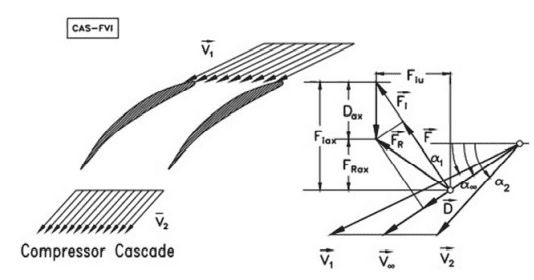
Starting from a given turbine cascade with the inlet and exit flow angles shown in Fig. 5.27, the blade force can be obtained by applying the linear momentum principles to the control volume with the unit normal vectors and the coordinate system shown in Fig. 5.27. Applying Eq. (5.26), the blade inviscid force is obtained from:
$$
\boldsymbol{F}i=\dot{m} \boldsymbol{V}_1-\dot{m} \boldsymbol{V}_2-\boldsymbol{n}_1 p_1 s h-\boldsymbol{n}_2 p_2 s h $$ with the subscript $i$ that refers to inviscid flow, $s$ as the spacing and $h$ as the blade height that can be assumed unity. The relationship between the control volume normal unit vectors and the unit vectors pertaining to the coordinate system is given by $\boldsymbol{n}_1=-\boldsymbol{e}_2$ and $\boldsymbol{n}_2=\boldsymbol{e}_2$. The velocities in Eq. (5.153) can be expressed in terms of circumferential as well as axial components: $$ \boldsymbol{F}_i=-e_1 \dot{m}\left[\left(V{u 1}+V_{u 2}\right)\right]+e_2\left[\dot{m}\left(V_{a x 1}-V_{a x 2}\right)+\left(p_1-p_2\right) s h\right]
$$
with $V_{a x 1}=V_{a x 2}$ as a result of incompressible flow assumption and $V_{u 1} \not \equiv V_{u 2}$ from Fig. 5.22. Equation (5.154) rearranged as:
$$
\boldsymbol{F}i=-\boldsymbol{e}_1 \dot{m}\left(V{u 1}+V_{u 2}\right)+\boldsymbol{e}2\left(p_1-p_2\right) s h=e_1 F_u+e_2 F{a x}
$$
with the circumferential and axial components
$$
F_u=-\dot{m}\left(V_{u 1}+V_{u 2}\right) \text { and } F_{a x}=\left(p_1-p_2\right) s h .
$$
The static pressure difference in Eq. (5.156) is obtained from the following Bernoulli equation:
$$
\begin{aligned}
p_{01} &=p_{02} \
p_1-p_2 &=\frac{1}{2} \rho\left(V_2^2-V_1^2\right)=\frac{1}{2} \rho\left(V_{u 2}^2-V_{u 1}^2\right) .
\end{aligned}
$$
Inserting the pressure difference along with the mass flow $\dot{m}=\rho V_{a x} s h$ into Eq. (5.156) and the blade height $h=1$, we obtain the axial as well as the circumferential components of the lift force:
$$
\left.\begin{array}{l}
F_{a x}=\frac{1}{2} \varrho\left(V_{u 2}+V_{u 1}\right)\left(V_{u 2}-V_{u 1}\right) s \
F_u=-\varrho V_{a x}\left(V_{u 2}+V_{u 1}\right) s
\end{array}\right}
$$
物理代写|流体力学代写Fluid Mechanics代考|Blade Forces in a Viscous Flow Field
The working fluids in turbomachinery, whether air, combustion gas, steam or other substances, are always viscous. The blades are subjected to the viscous flow and undergo shear stresses with no-slip condition on blades, casing and hub surfaces, resulting in boundary layer developments. Furthermore, the blades have certain definite trailing edge thicknesses. These thicknesses together with the boundary layer thickness, generate a spatially periodic wake flow downstream of each cascade as shown in Fig. 5.30.
The presence of the shear stresses cause drag forces that reduce the total pressure. In order to calculate the blade forces, the momentum Eq. (5.153) can be applied to the viscous flows. As seen from Eq. (5.156), the circumferential component remains unchanged. The axial component, however, changes in accordance with the pressure difference as shown in the following relations:
$$
\begin{aligned}
F_u &=-\rho V_{a x}\left(V_{u 2}+V_{u 1}\right) s h \
F_{a x} &=\left(p_1-p_2\right) s h .
\end{aligned}
$$
The blade height $h$ in Eq. (5.169) may be assumed as unity. For a viscous flow, the static pressure difference cannot be calculated by the Bernoulli equation. In this case, the total pressure drop must be taken into consideration. We define the total pressure loss coefficient:
$$
\zeta \equiv \frac{P_1-P_2}{\frac{1}{2} \varrho V_2^2}
$$
with $P_1$ and $P_2$ as the averaged total pressure at stations 1 and 2 . Inserting for the total pressure the sum of static and dynamic pressures, we get the static pressure difference as:
$$
p_1-p_2=\frac{\rho}{2}\left(V_2^2-V_1^2\right)+\zeta \frac{\rho}{2} V_2^2 .
$$
Incorporating Eq. (5.171) into the axial component of the blade force in Eq. (5.169) yields:
$$
F_{a x}=\frac{\rho}{2}\left(V_2^2-V_1^2\right) s+\zeta \frac{\rho}{2} V_2^2 s .
$$
We introduce the velocity components into Eq. (5.172) and assume that for an incompressible flow the axial components of the inlet and exit flows are the same. As a result, Eq. (5.172) reduces to:
$$
F_{a x}=\frac{\rho}{2}\left(V_{u 2}^2-V_{u 1}^2\right) s+\zeta \frac{\rho}{2} V_2^2 s .
$$
The second term on the right-hand side exhibits the axial component of drag forces accounting for the viscous nature of a frictional flow shown in Fig. 5.31. Thus, the axial projection of the drag force is obtained from:
$$
D_{a x}=\zeta \frac{\rho}{2} V_2^2 s
$$
流体力学代写
物理代写|流体力学代写流体力学代考|无粘流场中的叶片力
从图5.27所示的进气角和出气角给定的涡轮叶栅出发,将线性动量原理应用于控制体积,单位法向量,坐标系统如图5.27所示,可得到叶片力。应用式(5.26),得到叶片无粘力:
$$
\boldsymbol{F}i=\dot{m} \boldsymbol{V}1-\dot{m} \boldsymbol{V}_2-\boldsymbol{n}_1 p_1 s h-\boldsymbol{n}_2 p_2 s h $$,下标$i$表示无粘流量,$s$为间距,$h$为可统一假设的叶片高度。控制体积法单位向量与坐标系中的单位向量之间的关系由$\boldsymbol{n}_1=-\boldsymbol{e}_2$和$\boldsymbol{n}_2=\boldsymbol{e}_2$给出。式(5.153)中的速度可以用周向分量和轴向分量表示:由于不可压缩流动假设,$$ \boldsymbol{F}_i=-e_1 \dot{m}\left[\left(V{u 1}+V{u 2}\right)\right]+e_2\left[\dot{m}\left(V_{a x 1}-V_{a x 2}\right)+\left(p_1-p_2\right) s h\right]
$$
与$V_{a x 1}=V_{a x 2}$,图5.22中的$V_{u 1} \not \equiv V_{u 2}$。式(5.154)重新排列为:
$$
\boldsymbol{F}i=-\boldsymbol{e}1 \dot{m}\left(V{u 1}+V{u 2}\right)+\boldsymbol{e}2\left(p_1-p_2\right) s h=e_1 F_u+e_2 F{a x}
$$
,其中周向分量和轴向分量
$$
F_u=-\dot{m}\left(V_{u 1}+V_{u 2}\right) \text { and } F_{a x}=\left(p_1-p_2\right) s h .
$$
式(5.156)中的静压差由以下伯努利方程得到:< /p>
$$
\begin{aligned}
p_{01} &=p_{02} \
p_1-p_2 &=\frac{1}{2} \rho\left(V_2^2-V_1^2\right)=\frac{1}{2} \rho\left(V_{u 2}^2-V_{u 1}^2\right) .
\end{aligned}
$$
随着质量流量插入压差 $\dot{m}=\rho V_{a x} s h$ 式(5.156)和叶片高度 $h=1$,得到升力的轴向分量和周向分量:
$$
\left.\begin{array}{l}
F_{a x}=\frac{1}{2} \varrho\left(V_{u 2}+V_{u 1}\right)\left(V_{u 2}-V_{u 1}\right) s \
F_u=-\varrho V_{a x}\left(V_{u 2}+V_{u 1}\right) s
\end{array}\right}
$$
物理代写|流体力学代写流体力学代考|叶片在粘性流场中的力
叶轮机械中的工作流体,无论是空气、燃烧气体、蒸汽还是其他物质,总是粘性的。在叶片、机匣和轮毂表面无滑移的情况下,叶片受到粘性流动和剪切应力的作用,导致边界层发展。此外,叶片具有一定的后缘厚度。这些厚度与边界层厚度一起,在每个叶栅下游产生空间周期性尾流,如图5.30所示。剪切应力的存在会产生阻力,从而降低总压力。为了计算叶片力,可以将动量式(5.153)应用于粘性流动。由式(5.156)可知,周向分量不变。而轴向分量则随压差变化,其关系如下:
$$
\begin{aligned}
F_u &=-\rho V_{a x}\left(V_{u 2}+V_{u 1}\right) s h \
F_{a x} &=\left(p_1-p_2\right) s h .
\end{aligned}
$$
式(5.169)中的叶片高度$h$可以假设为单位。对于粘性流体,静压差不能用伯努利方程计算。在这种情况下,必须考虑总压降。我们定义总压损失系数:
$$
\zeta \equiv \frac{P_1-P_2}{\frac{1}{2} \varrho V_2^2}
$$
,其中$P_1$和$P_2$为1站和2站的平均总压。将总压力插入静态压力和动态压力之和,我们得到静压差为:
$$
p_1-p_2=\frac{\rho}{2}\left(V_2^2-V_1^2\right)+\zeta \frac{\rho}{2} V_2^2 .
$$
将Eq.(5.171)加入到Eq.(5.169)中叶片力的轴向分量中,得到:
$$
F_{a x}=\frac{\rho}{2}\left(V_2^2-V_1^2\right) s+\zeta \frac{\rho}{2} V_2^2 s .
$$
我们将速度分量引入Eq.(5.172)中,并假设对于不可压缩流动,进口和出口流动的轴向分量是相同的。因此,式(5.172)减少为:
$$
F_{a x}=\frac{\rho}{2}\left(V_{u 2}^2-V_{u 1}^2\right) s+\zeta \frac{\rho}{2} V_2^2 s .
$$
右边的第二项显示了摩擦力的轴向分量,这是图5.31所示的摩擦力流的粘性性质。因此,阻力的轴向投影由:
$$
D_{a x}=\zeta \frac{\rho}{2} V_2^2 s
$$
得到

统计代写请认准statistics-lab™. statistics-lab™为您的留学生涯保驾护航。
金融工程代写
金融工程是使用数学技术来解决金融问题。金融工程使用计算机科学、统计学、经济学和应用数学领域的工具和知识来解决当前的金融问题,以及设计新的和创新的金融产品。
非参数统计代写
非参数统计指的是一种统计方法,其中不假设数据来自于由少数参数决定的规定模型;这种模型的例子包括正态分布模型和线性回归模型。
广义线性模型代考
广义线性模型(GLM)归属统计学领域,是一种应用灵活的线性回归模型。该模型允许因变量的偏差分布有除了正态分布之外的其它分布。
术语 广义线性模型(GLM)通常是指给定连续和/或分类预测因素的连续响应变量的常规线性回归模型。它包括多元线性回归,以及方差分析和方差分析(仅含固定效应)。
有限元方法代写
有限元方法(FEM)是一种流行的方法,用于数值解决工程和数学建模中出现的微分方程。典型的问题领域包括结构分析、传热、流体流动、质量运输和电磁势等传统领域。
有限元是一种通用的数值方法,用于解决两个或三个空间变量的偏微分方程(即一些边界值问题)。为了解决一个问题,有限元将一个大系统细分为更小、更简单的部分,称为有限元。这是通过在空间维度上的特定空间离散化来实现的,它是通过构建对象的网格来实现的:用于求解的数值域,它有有限数量的点。边界值问题的有限元方法表述最终导致一个代数方程组。该方法在域上对未知函数进行逼近。[1] 然后将模拟这些有限元的简单方程组合成一个更大的方程系统,以模拟整个问题。然后,有限元通过变化微积分使相关的误差函数最小化来逼近一个解决方案。
tatistics-lab作为专业的留学生服务机构,多年来已为美国、英国、加拿大、澳洲等留学热门地的学生提供专业的学术服务,包括但不限于Essay代写,Assignment代写,Dissertation代写,Report代写,小组作业代写,Proposal代写,Paper代写,Presentation代写,计算机作业代写,论文修改和润色,网课代做,exam代考等等。写作范围涵盖高中,本科,研究生等海外留学全阶段,辐射金融,经济学,会计学,审计学,管理学等全球99%专业科目。写作团队既有专业英语母语作者,也有海外名校硕博留学生,每位写作老师都拥有过硬的语言能力,专业的学科背景和学术写作经验。我们承诺100%原创,100%专业,100%准时,100%满意。
随机分析代写
随机微积分是数学的一个分支,对随机过程进行操作。它允许为随机过程的积分定义一个关于随机过程的一致的积分理论。这个领域是由日本数学家伊藤清在第二次世界大战期间创建并开始的。
时间序列分析代写
随机过程,是依赖于参数的一组随机变量的全体,参数通常是时间。 随机变量是随机现象的数量表现,其时间序列是一组按照时间发生先后顺序进行排列的数据点序列。通常一组时间序列的时间间隔为一恒定值(如1秒,5分钟,12小时,7天,1年),因此时间序列可以作为离散时间数据进行分析处理。研究时间序列数据的意义在于现实中,往往需要研究某个事物其随时间发展变化的规律。这就需要通过研究该事物过去发展的历史记录,以得到其自身发展的规律。
回归分析代写
多元回归分析渐进(Multiple Regression Analysis Asymptotics)属于计量经济学领域,主要是一种数学上的统计分析方法,可以分析复杂情况下各影响因素的数学关系,在自然科学、社会和经济学等多个领域内应用广泛。
MATLAB代写
MATLAB 是一种用于技术计算的高性能语言。它将计算、可视化和编程集成在一个易于使用的环境中,其中问题和解决方案以熟悉的数学符号表示。典型用途包括:数学和计算算法开发建模、仿真和原型制作数据分析、探索和可视化科学和工程图形应用程序开发,包括图形用户界面构建MATLAB 是一个交互式系统,其基本数据元素是一个不需要维度的数组。这使您可以解决许多技术计算问题,尤其是那些具有矩阵和向量公式的问题,而只需用 C 或 Fortran 等标量非交互式语言编写程序所需的时间的一小部分。MATLAB 名称代表矩阵实验室。MATLAB 最初的编写目的是提供对由 LINPACK 和 EISPACK 项目开发的矩阵软件的轻松访问,这两个项目共同代表了矩阵计算软件的最新技术。MATLAB 经过多年的发展,得到了许多用户的投入。在大学环境中,它是数学、工程和科学入门和高级课程的标准教学工具。在工业领域,MATLAB 是高效研究、开发和分析的首选工具。MATLAB 具有一系列称为工具箱的特定于应用程序的解决方案。对于大多数 MATLAB 用户来说非常重要,工具箱允许您学习和应用专业技术。工具箱是 MATLAB 函数(M 文件)的综合集合,可扩展 MATLAB 环境以解决特定类别的问题。可用工具箱的领域包括信号处理、控制系统、神经网络、模糊逻辑、小波、仿真等。