如果你也在 怎样代写线性回归分析linear regression analysis这个学科遇到相关的难题,请随时右上角联系我们的24/7代写客服。
回归分析是一种强大的统计方法,允许你检查两个或多个感兴趣的变量之间的关系。虽然有许多类型的回归分析,但它们的核心都是考察一个或多个自变量对因变量的影响。
statistics-lab™ 为您的留学生涯保驾护航 在代写线性回归分析linear regression analysis方面已经树立了自己的口碑, 保证靠谱, 高质且原创的统计Statistics代写服务。我们的专家在代写线性回归分析linear regression analysis代写方面经验极为丰富,各种代写线性回归分析linear regression analysis相关的作业也就用不着说。
我们提供的线性回归分析linear regression analysis及其相关学科的代写,服务范围广, 其中包括但不限于:
- Statistical Inference 统计推断
- Statistical Computing 统计计算
- Advanced Probability Theory 高等楖率论
- Advanced Mathematical Statistics 高等数理统计学
- (Generalized) Linear Models 广义线性模型
- Statistical Machine Learning 统计机器学习
- Longitudinal Data Analysis 纵向数据分析
- Foundations of Data Science 数据科学基础
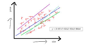
统计代写|线性回归分析代写linear regression analysis代考|The MLR Model
Definition 2.1. The response variable is the variable that you want to predict. The predictor variables are the variables used to predict the response variable.
Notation. In this text the response variable will usually be denoted by $Y$ and the $p$ predictor variables will often be denoted by $x_1, \ldots, x_p$. The response variable is also called the dependent variable while the predictor variables are also called independent variables, explanatory variables, carriers, or covariates. Often the predictor variables will be collected in a vector $\boldsymbol{x}$. Then $\boldsymbol{x}^T$ is the transpose of $\boldsymbol{x}$.
Definition 2.2. Regression is the study of the conditional distribution $Y \mid \boldsymbol{x}$ of the response variable $Y$ given the vector of predictors $\boldsymbol{x}=$ $\left(x_1, \ldots, x_p\right)^T$.
Definition 2.3. A quantitative variable takes on numerical values while a qualitative variable takes on categorical values.
Example 2.1. Archeologists and crime scene investigators sometimes want to predict the height of a person from partial skeletal remains. A model for prediction can be built from nearly complete skeletons or from living humans, depending on the population of interest (e.g., ancient Egyptians or modern US citizens). The response variable $Y$ is height and the predictor variables might be $x_1 \equiv 1, x_2=$ femur length, and $x_3=u$ lna length.
The heights of individuals with $x_2=200 \mathrm{~mm}$ and $x_3=140 \mathrm{~mm}$ should be shorter on average than the heights of individuals with $x_2=500 \mathrm{~mm}$ and $x_3=350 \mathrm{~mm}$. In this example $Y, x_2$, and $x_3$ are quantitative variables. If $x_4=$ gender is a predictor variable, then gender (coded as male $=1$ and female $=0$ ) is qualitative.
统计代写|线性回归分析代写linear regression analysis代考|Checking Goodness of Fit
It is crucial to realize that an MLR model is not necessarily a useful model for the data, even if the data set consists of a response variable and several predictor variables. For example, a nonlinear regression model or a much more complicated model may be needed. Chapters 1 and 13 describe several alternative models. Let $p$ be the number of predictors and $n$ the number of cases. Assume that $n \geq 5 p$, then plots can be used to check whether the MLR model is useful for studying the data. This technique is known as checking the goodness of fit of the MLR model.
Notation. Plots will be used to simplify regression analysis, and in this text a plot of $W$ versus $Z$ uses $W$ on the horizontal axis and $Z$ on the vertical axis.
Definition 2.10. A scatterplot of $X$ versus $Y$ is a plot of $X$ versus $Y$ and is used to visualize the conditional distribution $Y \mid X$ of $Y$ given $X$.
Definition 2.11. A response plot is a plot of a variable $w_i$ versus $Y_i$. Typically $w_i$ is a linear combination of the predictors: $w_i=\boldsymbol{x}_i^T \boldsymbol{\eta}$ where $\boldsymbol{\eta}$ is a known $p \times 1$ vector. The most commonly used response plot is a plot of the fitted values $\widehat{Y}_i$ versus the response $Y_i$.
Proposition 2.1. Suppose that the regression estimator $\boldsymbol{b}$ of $\boldsymbol{\beta}$ is used to find the residuals $r_i \equiv r_i(\boldsymbol{b})$ and the fitted values $\widehat{Y}_i \equiv \widehat{Y}_i(\boldsymbol{b})=\boldsymbol{x}_i^T \boldsymbol{b}$. Then in the response plot of $\widehat{Y}_i$ versus $Y_i$, the vertical deviations from the identity line (that has unit slope and zero intercept) are the residuals $r_i(b)$.
Proof. The identity line in the response plot is $Y=\boldsymbol{x}^T \boldsymbol{b}$. Hence the vertical deviation is $Y_i-\boldsymbol{x}_i^T \boldsymbol{b}=r_i(\boldsymbol{b})$.
Definition 2.12. A residual plot is a plot of a variable $w_i$ versus the residuals $r_i$. The most commonly used residual plot is a plot of $\hat{Y}_i$ versus $r_i$.
Notation: For MLR, “the residual plot” will often mean the residual plot of $\hat{Y}_i$ versus $r_i$, and “the response plot” will often mean the plot of $\hat{Y}_i$ versus $Y_i$.
If the unimodal MLR model as estimated by least squares is useful, then in the response plot the plotted points should scatter about the identity line while in the residual plot of $\hat{Y}$ versus $r$ the plotted points should scatter about the $r=0$ line (the horizontal axis) with no other pattern. Figures 1.2 and 1.3 show what a response plot and residual plot look like for an artificial MLR data set where the MLR regression relationship is rather strong in that the sample correlation $\operatorname{corr}(\hat{Y}, Y)$ is near 1. Figure 1.4 shows a response plot where the response $Y$ is independent of the nontrivial predictors in the model. Here $\operatorname{corr}(\hat{Y}, Y)$ is near 0 but the points still scatter about the identity line. When the MLR relationship is very weak, the response plot will look like the residual plot.
线性回归代写
统计代写|线性回归分析代写linear regression analysis代考|The MLR Model
定义 2.1。响应变量是您要预测的变量。预测变量是用于预测响应变量的变量。
符号。在本文中,响应变量通常表示为 $Y$ 和 $p$ 预测变量通常表示为 $x_1, \ldots, x_p$. 响应变量也称为因变量,而 预测变量也称为自变量、解释变量、载体或协变量。通常预测变量将收集在一个向量中 $\boldsymbol{x}$. 然后 $\boldsymbol{x}^T$ 是转置 $\boldsymbol{x}$.
定义 2.2。回归是对条件分布的研究 $Y \mid \boldsymbol{x}$ 响应变量 $Y$ 给定预测变量向量 $\boldsymbol{x}=\left(x_1, \ldots, x_p\right)^T$.
定义 2.3。定量变量采用数值,而定性变量采用分类值。
示例 2.1。考古学家和犯罪现场调查员有时想根据部分骨骼遗骸来预测一个人的身高。根据感兴趣的人群 (例如,古埃及人或现代美国公民),可以从几乎完整的骨骼或活人中构建预测模型。响应变量 $Y$ 是高 度,预测变量可能是 $x_1 \equiv 1, x_2=$ 股骨长度,和 $x_3=u$ Ina长度。
个人的身高 $x_2=200 \mathrm{~mm}$ 和 $x_3=140 \mathrm{~mm}$ 平均身高应该比有 $x_2=500 \mathrm{~mm}$ 和 $x_3=350 \mathrm{~mm}$. 在这 个例子中 $Y, x_2$ ,和 $x_3$ 是定量变量。如果 $x_4=$ 性别是预测变量,然后性别 (编码为男性 $=1$ 和女性 $=0$ ) 是定性的。
统计代写|线性回归分析代写linear regression analysis代考|Checking Goodness of Fit
重要的是要认识到 MLR 模型不一定是对数据有用的模型,即使数据集由一个响应变量和几个预测变量组 成。例如,可能需要非线性回归模型或更复杂的模型。第 1 章和第 13 章描述了几种替代模型。让 $p$ 是预测 变量的数量和 $n$ 案件的数量。假使,假设 $n \geq 5 p$ ,然后可以使用图来检查 MLR 模型是否对研究数据有 用。这种技术称为检查 MLR 模型的拟合优度。
符号。绘图将用于简化回归分析,在本文中的绘图 $W$ 相对 $Z$ 使用 $W$ 在水平轴上和 $Z$ 在垂直轴上。
定义 2.10。的散点图 $X$ 相对 $Y$ 是一个情节 $X$ 相对 $Y$ 并用于可视化条件分布 $Y \mid X$ 的 $Y$ 给予 $X$.
定义 2.11。响应图是变量图 $w_i$ 相对 $Y_i$. 通常 $w_i$ 是预测变量的线性组合: $w_i=\boldsymbol{x}_i^T \boldsymbol{\eta}$ 在哪里 $\boldsymbol{\eta}$ 是一个已知 的 $p \times 1$ 向量。最常用的响应图是拟合值图 $\widehat{Y}_i$ 与响应 $Y_i$.
提案 2.1。假设回归估计 $\boldsymbol{b}$ 的 $\boldsymbol{\beta}$ 用于查找残差 $r_i \equiv r_i(\boldsymbol{b})$ 和拟合值 $\widehat{Y}_i \equiv \widehat{Y}_i(\boldsymbol{b})=\boldsymbol{x}_i^T \boldsymbol{b}$. 然后在响应图中 $\widehat{Y}_i$ 相对 $Y_i$ ,与标识线 (具有单位斜率和零截距) 的垂直偏差是残差 $r_i(b)$.
证明。响应图中的身份线是 $Y=\boldsymbol{x}^T \boldsymbol{b}$. 因此垂直偏差是 $Y_i-\boldsymbol{x}_i^T \boldsymbol{b}=r_i(\boldsymbol{b})$.
定义 2.12。残差图是变量图 $w_i$ 与残差 $r_i$. 最常用的残差图是 $\hat{Y}_i$ 相对 $r_i$.
如果通过最小二乘法估计的单峰 MLR 模型是有用的,那么在响应图中,标绘点应该散布在标识线上,而 在残差图中 $\hat{Y}$ 相对 $r$ 绘制的点应该散布在 $r=0$ 没有其他图案的线(水平轴)。图 1.2 和 1.3 显示了人工 MLR 数据集的响应图和残差图的样子,其中 MLR 回归关系相当强,因为样本相关性 $\operatorname{corr}(\hat{Y}, Y)$ 接近 1 。 图 1.4 显示了一个响应图,其中响应 $Y$ 独立于模型中的非平凡预测变量。这里 $\operatorname{corr}(\hat{Y}, Y)$ 接近 0 ,但点仍 然散布在标识线上。当 MLR 关系非常弱时,响应图看起来像残差图。

统计代写请认准statistics-lab™. statistics-lab™为您的留学生涯保驾护航。
随机过程代考
在概率论概念中,随机过程是随机变量的集合。 若一随机系统的样本点是随机函数,则称此函数为样本函数,这一随机系统全部样本函数的集合是一个随机过程。 实际应用中,样本函数的一般定义在时间域或者空间域。 随机过程的实例如股票和汇率的波动、语音信号、视频信号、体温的变化,随机运动如布朗运动、随机徘徊等等。
贝叶斯方法代考
贝叶斯统计概念及数据分析表示使用概率陈述回答有关未知参数的研究问题以及统计范式。后验分布包括关于参数的先验分布,和基于观测数据提供关于参数的信息似然模型。根据选择的先验分布和似然模型,后验分布可以解析或近似,例如,马尔科夫链蒙特卡罗 (MCMC) 方法之一。贝叶斯统计概念及数据分析使用后验分布来形成模型参数的各种摘要,包括点估计,如后验平均值、中位数、百分位数和称为可信区间的区间估计。此外,所有关于模型参数的统计检验都可以表示为基于估计后验分布的概率报表。
广义线性模型代考
广义线性模型(GLM)归属统计学领域,是一种应用灵活的线性回归模型。该模型允许因变量的偏差分布有除了正态分布之外的其它分布。
statistics-lab作为专业的留学生服务机构,多年来已为美国、英国、加拿大、澳洲等留学热门地的学生提供专业的学术服务,包括但不限于Essay代写,Assignment代写,Dissertation代写,Report代写,小组作业代写,Proposal代写,Paper代写,Presentation代写,计算机作业代写,论文修改和润色,网课代做,exam代考等等。写作范围涵盖高中,本科,研究生等海外留学全阶段,辐射金融,经济学,会计学,审计学,管理学等全球99%专业科目。写作团队既有专业英语母语作者,也有海外名校硕博留学生,每位写作老师都拥有过硬的语言能力,专业的学科背景和学术写作经验。我们承诺100%原创,100%专业,100%准时,100%满意。
机器学习代写
随着AI的大潮到来,Machine Learning逐渐成为一个新的学习热点。同时与传统CS相比,Machine Learning在其他领域也有着广泛的应用,因此这门学科成为不仅折磨CS专业同学的“小恶魔”,也是折磨生物、化学、统计等其他学科留学生的“大魔王”。学习Machine learning的一大绊脚石在于使用语言众多,跨学科范围广,所以学习起来尤其困难。但是不管你在学习Machine Learning时遇到任何难题,StudyGate专业导师团队都能为你轻松解决。
多元统计分析代考
基础数据: $N$ 个样本, $P$ 个变量数的单样本,组成的横列的数据表
变量定性: 分类和顺序;变量定量:数值
数学公式的角度分为: 因变量与自变量
时间序列分析代写
随机过程,是依赖于参数的一组随机变量的全体,参数通常是时间。 随机变量是随机现象的数量表现,其时间序列是一组按照时间发生先后顺序进行排列的数据点序列。通常一组时间序列的时间间隔为一恒定值(如1秒,5分钟,12小时,7天,1年),因此时间序列可以作为离散时间数据进行分析处理。研究时间序列数据的意义在于现实中,往往需要研究某个事物其随时间发展变化的规律。这就需要通过研究该事物过去发展的历史记录,以得到其自身发展的规律。
回归分析代写
多元回归分析渐进(Multiple Regression Analysis Asymptotics)属于计量经济学领域,主要是一种数学上的统计分析方法,可以分析复杂情况下各影响因素的数学关系,在自然科学、社会和经济学等多个领域内应用广泛。
MATLAB代写
MATLAB 是一种用于技术计算的高性能语言。它将计算、可视化和编程集成在一个易于使用的环境中,其中问题和解决方案以熟悉的数学符号表示。典型用途包括:数学和计算算法开发建模、仿真和原型制作数据分析、探索和可视化科学和工程图形应用程序开发,包括图形用户界面构建MATLAB 是一个交互式系统,其基本数据元素是一个不需要维度的数组。这使您可以解决许多技术计算问题,尤其是那些具有矩阵和向量公式的问题,而只需用 C 或 Fortran 等标量非交互式语言编写程序所需的时间的一小部分。MATLAB 名称代表矩阵实验室。MATLAB 最初的编写目的是提供对由 LINPACK 和 EISPACK 项目开发的矩阵软件的轻松访问,这两个项目共同代表了矩阵计算软件的最新技术。MATLAB 经过多年的发展,得到了许多用户的投入。在大学环境中,它是数学、工程和科学入门和高级课程的标准教学工具。在工业领域,MATLAB 是高效研究、开发和分析的首选工具。MATLAB 具有一系列称为工具箱的特定于应用程序的解决方案。对于大多数 MATLAB 用户来说非常重要,工具箱允许您学习和应用专业技术。工具箱是 MATLAB 函数(M 文件)的综合集合,可扩展 MATLAB 环境以解决特定类别的问题。可用工具箱的领域包括信号处理、控制系统、神经网络、模糊逻辑、小波、仿真等。