如果你也在 怎样代写线性回归Linear Regression 这个学科遇到相关的难题,请随时右上角联系我们的24/7代写客服。线性回归Linear Regression在统计学中,是对标量响应和一个或多个解释变量(也称为因变量和自变量)之间的关系进行建模的一种线性方法。一个解释变量的情况被称为简单线性回归;对于一个以上的解释变量,这一过程被称为多元线性回归。这一术语不同于多元线性回归,在多元线性回归中,预测的是多个相关的因变量,而不是一个标量变量。
线性回归Linear Regression在线性回归中,关系是用线性预测函数建模的,其未知的模型参数是根据数据估计的。最常见的是,假设给定解释变量(或预测因子)值的响应的条件平均值是这些值的仿生函数;不太常见的是,使用条件中位数或其他一些量化指标。像所有形式的回归分析一样,线性回归关注的是给定预测因子值的反应的条件概率分布,而不是所有这些变量的联合概率分布,这是多元分析的领域。
statistics-lab™ 为您的留学生涯保驾护航 在代写线性回归分析linear regression analysis方面已经树立了自己的口碑, 保证靠谱, 高质且原创的统计Statistics代写服务。我们的专家在代写线性回归分析linear regression analysis代写方面经验极为丰富,各种代写线性回归分析linear regression analysis相关的作业也就用不着说。
Historically, researchers commonly used a test known as the “Durbin-Watson test” to test for the first-order autocorrelation in pure time-series data. Currently, many tests other than the Durbin-Watson test, such as likelihood ratio tests, are supplied routinely by software that can analyze time-series data. An even simpler (but still useful) test to discover whether the trend in the $\left(e_{t-1}, e_t\right)$ plot (the right panel of Figures 4.8) is explainable by chance alone is given by the cor.test function in R. Simply specify cor. test(resid, lag.resid) to get the result. For the Car Sales data you get the following output:
$$
\text { Pearson’s product-moment correlation }
$$
data: resid and laq.resid
$t=9.4162$, df $=117$, p-value $=5.175 \mathrm{e}-16$
alternative hypothesis: true correlation is not equal to 0
95 percent confidence interval:
0.5404718 0.7481668
sample estimates:
cor
0.6565924
Pearson’s product-moment correlation
data: resid and laq.resid
$t=9.4162, \mathrm{df}=117, \mathrm{p}$-value $=5.175 \mathrm{e}-16$
alternative hypothesis: true correlation is not equal to 0
95 percent confidence interval:
0.54047180 .7481668
sample estimates:
$\operatorname{cor}$
0.6565924
Notice that the estimated correlation is 0.6565924 , a positive number, corroborating the positive linear trend shown in the right-hand panel of Figure 4.8. The $p$-value is $5.175 \times 10^{-16}$, indicating that the difference between 0.6565924 and 0.0 is nearly impossible to explain by chance alone. In other words, you will never (for all intents and purposes) see a trend as extreme as in Figure 4.8 in similarly-sized data sets $(n=120)$ that are produced by a model where the errors are in fact uncorrelated.
As always, you should identify a subject matter rationale for any claimed violation of an assumption. In this case, persistent macroeconomic conditions explain that the Sales residual (deviation from Sales prediction based on the interest rate) in a given month is quite similar to that of a previous month, but not so similar to five years ago. In other words, if conditions in the U.S. economy cause higher sales than expected (given interest rates) this month, such conditions are likely to persist through next month, also causing higher sales.
统计代写|线性回归分析代写linear regression analysis代考|Evaluating the Normality Assumption Using Graphical Methods
The normality assumption states that each conditional distribution $p(y \mid x)$ (one for each $x$ ) is a normal distribution. The normality assumption does not state that the marginal distribution $p(y)$ is normal. It is possible that the distributions $p(y \mid x)$ are all normal yet the distribution $p(y)$ is non-normal; this happens when the distribution of $X$ is non-normal. Thus, you do not assess the normality assumption using the $y_i$ data alone. You have to consider the data $Y$ within specific $X=x$ values.
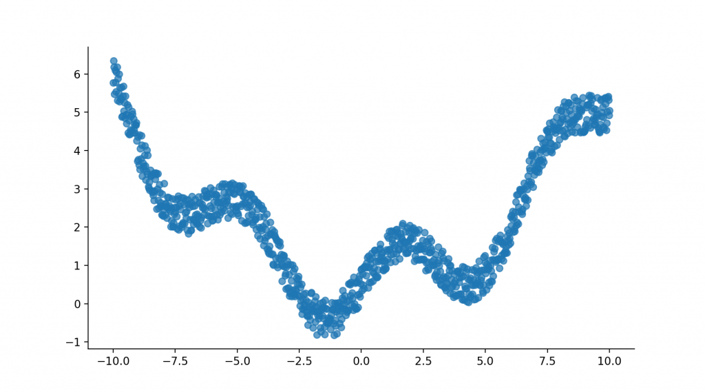
It is a common error of statistical practice to check normality using the $y_i$ data, so we wish to clarify this issue first, before showing proper methods. Consider a regression process where $Y \mid X=x$ is normal for all $X=x$, with mean $10+2 x$ and variance 1.0 , but where $X$ has the exponential distribution with mean 1.0. The following code generates 200 observations from such a process and shows the $q-q$ plot of the $y_i$ data values. Despite all of the assumptions being satisfied, including normality, the $q-q$ plot in Figure 4.9 incorrectly suggests that the normality assumption is violated.
R code for Figure 4.9
# Normal conditional distributions,
$#$ but non-normal marginal distribution
$X=$ rexp $(200,1)$
$# \mathrm{Y}$ is conditionally normal with mean $=10+2 \mathrm{x}$ and variance $=1$
$Y=10+2 * X+\operatorname{rnorm}(200)$
qqnorm(Y); qqline( $Y)$
# Normal conditional distributions,
# but non-normal marginal distribution
$\mathrm{X}=\operatorname{rexp}(200,1)$
# $Y$ is conditionally normal with mean $=10+2 x$ and variance=1
$Y=10+2 \star X+\operatorname{rnorm}(200)$
qquorm $(Y) ; q q l i n e(Y)$

线性回归代写
要评估不相关误差假设,首先必须考虑数据集的类型,是纯时间序列、横断面时间序列、空间、重复测量还是多层(分组)数据。对于纯时间序列数据,通常使用$t$而不是$i$表示观测指标,通常使用$T$而不是$n$表示数据集中的时间点数量,因此观测集是通过$t=1,2, \ldots, T$而不是$i=1,2, \ldots, n$进行索引的。
在纯时间序列过程中,不相关误差假设经常被严重违反,因为,例如,今天与昨天相似,但与五年前不太相似。因此,今天的误差项$\varepsilon_t$的潜在可观察值通常与昨天的误差项$\varepsilon_{t-1}$的潜在可观察值高度相关,这意味着违反了不相关误差假设。
要诊断纯时间序列数据的相关错误,您应该首先检查时间序列残差图,或$\left(t, e_t\right)$。寻找系统的、非随机的模式,如趋势或正弦波类型的功能模式,以表明这种假设的失败。这张图的完全随机外观与不相关的误差是一致的。
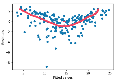
最常见的残差相关性类型是当前误差$\varepsilon_t$与先前误差$\varepsilon_{t-1}$的相关性,这被称为“滞后”误差项。这种相关性被称为自相关,因为它指的是变量与自身的相关性。因此,您可以查看的第二个图是滞后散点图,或$\left(e_{t-1}, e_t\right)$,您可以在其上叠加OLS或黄土拟合来查看趋势。该图中的趋势表明当前残差与前一个残差之间存在依赖关系,这违反了不相关误差假设。没有趋势的随机散点与不相关误差是一致的。
第三种图是残差的自相关函数,它显示滞后1、$\operatorname{lag} 2$、滞后3和更多的自相关性,因此您可以使用这种图来检查滞后大于1的自相关性。
对于非纯时间序列数据,需要不同的方法。对于空间数据(“空间”中的点,例如,具有地理坐标的数据),您可以使用变异图来检查误差相关性,在这种情况下称为“空间自相关性”。对于多水平(分组)数据,您可以检查散点图,其中数据按组标记以诊断相关性结构;第十章涉及这个问题。现在,我们只讨论纯时间序列数据。
统计代写|线性回归分析代写linear regression analysis代考|Evaluating the Normality Assumption Using Graphical Methods
Car Sales数据是纯时间序列,因为数据是连续120个月收集的。下面的代码显示了检查不相关(特别是非自相关)错误的相关图。
CarS = read.table(“https://raw.githubusercontent.com/andrea2719/ .table “)
“URA-DataSets/master/Cars.txt”)
attach(CarS);$\mathrm{n}=$ nrow(CarS)
fit $=$ lm(NSOLD $~$ INTRATE)
Resid $=$ fit$残差
par(mfrow=c(1,2))
图($1: n$, resid, xlab=”month”, ylab=”residual”)
点数($1: n$, resid, type=”l”);abline(h=0)
滞后。resid = c(NA, resid[1:n-1])
情节(滞后)Resid, Resid, xlab=”滞后残差”,ylab= “残差”)
abline(lsfit);残留,残留))
汽车$=$阅读。表$($”https://raw.githubusercontent。com andrea $2719 /$
“URA-DataSets/master/Cars.txt”)
附件(汽车);$n=\operatorname{nrow}(\operatorname{Cars})$
$\mathrm{fit}=\operatorname{lm}(\mathrm{NSOLD} \sim$ INTRATE $)$
Resid $=$ fit$残差
Par (mfrow=c $(1,2))$
图($1: n$,残差,$x l a b=$“月”,ylab=“残差”)
points $(1: \mathrm{n}$, resid, type=”I”);在线$(\mathrm{h}=0)$
滞后。渣油$=c(N A, r e s i d[1: n-1])$
情节滞后。Resid, Resid, $x l a b=$ “滞后残差”,ylab = “残差”)
Abline (lsfit (lag))残留,残留))
结果如图4.8所示。这两幅图都显示了大量的自相关证据。
这种极端违反假设的后果是什么?根据第3章中总结的数学定理,如果数据生成过程确实由回归模型给出,那么置信区间和$p$ -值的行为精确地与广告一样,精确地具有95%的置信度,精确地具有5%的显著性水平。如图所示,当独立性假设严重违反时,真实的置信水平可能远低于95%,真实的显著性水平可能远低于5%。有多远?你猜对了:你可以通过模拟来找到答案。

统计代写请认准statistics-lab™. statistics-lab™为您的留学生涯保驾护航。
随机过程代考
在概率论概念中,随机过程是随机变量的集合。 若一随机系统的样本点是随机函数,则称此函数为样本函数,这一随机系统全部样本函数的集合是一个随机过程。 实际应用中,样本函数的一般定义在时间域或者空间域。 随机过程的实例如股票和汇率的波动、语音信号、视频信号、体温的变化,随机运动如布朗运动、随机徘徊等等。
贝叶斯方法代考
贝叶斯统计概念及数据分析表示使用概率陈述回答有关未知参数的研究问题以及统计范式。后验分布包括关于参数的先验分布,和基于观测数据提供关于参数的信息似然模型。根据选择的先验分布和似然模型,后验分布可以解析或近似,例如,马尔科夫链蒙特卡罗 (MCMC) 方法之一。贝叶斯统计概念及数据分析使用后验分布来形成模型参数的各种摘要,包括点估计,如后验平均值、中位数、百分位数和称为可信区间的区间估计。此外,所有关于模型参数的统计检验都可以表示为基于估计后验分布的概率报表。
广义线性模型代考
广义线性模型(GLM)归属统计学领域,是一种应用灵活的线性回归模型。该模型允许因变量的偏差分布有除了正态分布之外的其它分布。
statistics-lab作为专业的留学生服务机构,多年来已为美国、英国、加拿大、澳洲等留学热门地的学生提供专业的学术服务,包括但不限于Essay代写,Assignment代写,Dissertation代写,Report代写,小组作业代写,Proposal代写,Paper代写,Presentation代写,计算机作业代写,论文修改和润色,网课代做,exam代考等等。写作范围涵盖高中,本科,研究生等海外留学全阶段,辐射金融,经济学,会计学,审计学,管理学等全球99%专业科目。写作团队既有专业英语母语作者,也有海外名校硕博留学生,每位写作老师都拥有过硬的语言能力,专业的学科背景和学术写作经验。我们承诺100%原创,100%专业,100%准时,100%满意。
机器学习代写
随着AI的大潮到来,Machine Learning逐渐成为一个新的学习热点。同时与传统CS相比,Machine Learning在其他领域也有着广泛的应用,因此这门学科成为不仅折磨CS专业同学的“小恶魔”,也是折磨生物、化学、统计等其他学科留学生的“大魔王”。学习Machine learning的一大绊脚石在于使用语言众多,跨学科范围广,所以学习起来尤其困难。但是不管你在学习Machine Learning时遇到任何难题,StudyGate专业导师团队都能为你轻松解决。
多元统计分析代考
基础数据: $N$ 个样本, $P$ 个变量数的单样本,组成的横列的数据表
变量定性: 分类和顺序;变量定量:数值
数学公式的角度分为: 因变量与自变量
时间序列分析代写
随机过程,是依赖于参数的一组随机变量的全体,参数通常是时间。 随机变量是随机现象的数量表现,其时间序列是一组按照时间发生先后顺序进行排列的数据点序列。通常一组时间序列的时间间隔为一恒定值(如1秒,5分钟,12小时,7天,1年),因此时间序列可以作为离散时间数据进行分析处理。研究时间序列数据的意义在于现实中,往往需要研究某个事物其随时间发展变化的规律。这就需要通过研究该事物过去发展的历史记录,以得到其自身发展的规律。
回归分析代写
多元回归分析渐进(Multiple Regression Analysis Asymptotics)属于计量经济学领域,主要是一种数学上的统计分析方法,可以分析复杂情况下各影响因素的数学关系,在自然科学、社会和经济学等多个领域内应用广泛。
MATLAB代写
MATLAB 是一种用于技术计算的高性能语言。它将计算、可视化和编程集成在一个易于使用的环境中,其中问题和解决方案以熟悉的数学符号表示。典型用途包括:数学和计算算法开发建模、仿真和原型制作数据分析、探索和可视化科学和工程图形应用程序开发,包括图形用户界面构建MATLAB 是一个交互式系统,其基本数据元素是一个不需要维度的数组。这使您可以解决许多技术计算问题,尤其是那些具有矩阵和向量公式的问题,而只需用 C 或 Fortran 等标量非交互式语言编写程序所需的时间的一小部分。MATLAB 名称代表矩阵实验室。MATLAB 最初的编写目的是提供对由 LINPACK 和 EISPACK 项目开发的矩阵软件的轻松访问,这两个项目共同代表了矩阵计算软件的最新技术。MATLAB 经过多年的发展,得到了许多用户的投入。在大学环境中,它是数学、工程和科学入门和高级课程的标准教学工具。在工业领域,MATLAB 是高效研究、开发和分析的首选工具。MATLAB 具有一系列称为工具箱的特定于应用程序的解决方案。对于大多数 MATLAB 用户来说非常重要,工具箱允许您学习和应用专业技术。工具箱是 MATLAB 函数(M 文件)的综合集合,可扩展 MATLAB 环境以解决特定类别的问题。可用工具箱的领域包括信号处理、控制系统、神经网络、模糊逻辑、小波、仿真等。