如果你也在 怎样代写微观经济学Microeconomics这个学科遇到相关的难题,请随时右上角联系我们的24/7代写客服。
微观经济学是研究稀缺性及其对资源的使用、商品和服务的生产、生产和福利的长期增长的影响,以及对社会至关重要的其他大量复杂问题的研究。
statistics-lab™ 为您的留学生涯保驾护航 在代写微观经济学Microeconomics方面已经树立了自己的口碑, 保证靠谱, 高质且原创的统计Statistics代写服务。我们的专家在代写微观经济学Microeconomics代写方面经验极为丰富,各种代写微观经济学Microeconomics相关的作业也就用不着说。
我们提供的微观经济学Microeconomics及其相关学科的代写,服务范围广, 其中包括但不限于:
- Statistical Inference 统计推断
- Statistical Computing 统计计算
- Advanced Probability Theory 高等概率论
- Advanced Mathematical Statistics 高等数理统计学
- (Generalized) Linear Models 广义线性模型
- Statistical Machine Learning 统计机器学习
- Longitudinal Data Analysis 纵向数据分析
- Foundations of Data Science 数据科学基础
经济代写|微观经济学代写Microeconomics代考|The CES Utility Function
It follows that $\varrho=(\xi-1) / \xi$ and therefore another way to write a CES function that makes its elasticity of substitution explicit is
$$
\left(a_1 x_1^{(\xi-1) / \xi}+a_2 x_2^{(\xi-1) / \xi}\right)^{\xi /(\xi-1)} .
$$
The CES function, invented to be used as a production function, is homogeneous of degree 1: the easy proof is left to the reader. When $a_1=a_2=1$, a monotonic transformation sometimes used which is not homogeneous of degree 1 but is very simple to use is
$$
x_1^\delta / \delta+x_2^\delta / \delta .
$$
Its elasticity of substitution is, again, constant and given by $\xi=1 /(1-\delta)$.
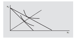
As one lets $Q$ vary, the CES approaches other well-known types of utility functions. For $\varrho$ tending to 1 from below, the elasticity of substitution tends to $+\infty$, that is, to the case of perfect substitutes. Indeed if one sets $Q=1$, one obtains the separable additive utility function of perfect substitutes, $u=a_1 x_1+a_2 x_2$. As $\varrho$ decreases, the elasticity of substitution decreases too, tending to 1 as $\varrho$ tends towards zero.
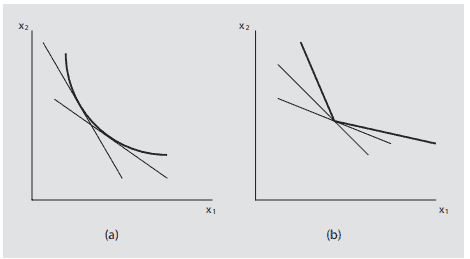
For $\varrho=0$ the CES function is not defined owing to division by zero, but if one lets $\varrho$ tend to 0 , the CES tends in the limit to have indifference curves identical to those of a Cobb-Douglas. Indeed, if $\varrho$ tends to zero the MRS tends to $-a_1 x_2 /\left(a_2 x_1\right)$ which is the same as for the generalized Cobb-Douglas $x_1{ }^\alpha x_2{ }^\beta$.
For $\varrho$ tending to $-\infty$ the indifference curves approach the L-shaped indifference curves of the case of perfect complementarity. ${ }^{35}$ The MRS, $-\left(a_1 / a_2\right) \cdot\left(x_2 /\right.$ $\left.x_1\right)^{1-e}$, tends to $-\left(a_1 / a_2\right) \cdot\left(x_2 / x_1\right)^{\infty}$ which has value $-\infty$ if $x_2>x_1$, zero if $x_2<x_1$; thus, indifference curves tend to become L-shaped with the corners on the $45^{\circ}$ straight line through the origin (which can always be obtained with an opportune choice of units for the goods).
经济代写|微观经济学代写Microeconomics代考|The Slutsky Equation
We finally tackle the issue of how the (Marshallian) demand for a good reacts to changes in prices. All the functions to appear below are assumed continuously differentiable, indifference curves are strictly convex, and the initial consumer choice is an interior basket, $x \gg 0$.
Let $\mathbf{p}^, m^$ be prices and income in the initial situation, and let $u^=v\left(\mathbf{p}^\right.$, $\left.m^\right)=u\left(\mathbf{x}\left(\mathbf{p}^, m^\right)\right), x_j^=x_j\left(\mathbf{p}^, m^\right)$. Differentiate both sides of $h_f(\mathbf{p}, u)=x_i(\mathbf{p}$, $e(\mathbf{p}, u))=x_i(\mathbf{p}, m)$ with respect to $p_j$
$$
\frac{\partial h_i\left(\mathbf{p}^, u^\right)}{\partial p_j}=\frac{\partial x_i\left(\mathbf{p}^, m^\right)}{\partial p_j}+\frac{\partial x_i\left(\mathbf{p}^, m^\right)}{\partial e\left(\mathbf{p}^, u^\right)} \cdot \frac{\partial e\left(\mathbf{p}^, u^\right)}{\partial p_j},
$$
where $\frac{\partial x_i\left(\mathbf{p}^, m^\right)}{\partial e\left(p^, u^\right)}$ can also be written $\frac{\partial x_i\left(\mathbf{p}^, m^\right)}{\partial m^}$, because initially $m=m^=e\left(\mathbf{p}^, u^\right)$ and under a balanced budget a variation in expenditure is the same thing as a variation in income. Furthermore, by Shephard’s Lemma $\partial e\left(\mathbf{p}^, u^\right) / \partial p_j=h_j\left(\mathbf{p}^, u^\right)$ $=x_j\left(\mathbf{p}^, e\left(\mathbf{p}^, u^\right)\right)=x_j^$. Hence
$$
\frac{\partial h_i\left(\mathbf{p}^, u^\right)}{\partial p_j}=\frac{\partial x_i\left(\mathbf{p}^, m^\right)}{\partial p_j}+\frac{\partial x_i\left(\mathbf{p}^, m^\right)}{\partial m} \cdot x_j^* .
$$
Let us indicate as $S(\mathbf{p}, m) \equiv\left[s_{i j}\right]$ the $n \times n$ Jacobian matrix of the vector of Hicksian demand functions for individual goods which form $\mathbf{h}(\mathbf{p}, u)$. Element $(i, j)$ of this matrix is
$$
s_{i j}=\frac{\partial h_i\left(\mathbf{p}^, u^\right)}{\partial p_j},
$$
for which equality (4.6) holds. Matrix $S(\mathbf{p}, m) \equiv\left[s_{i j}\right]$ is called Slutsky matrix or also matrix of Hicksian substitution effects. It yields
$$
\mathrm{dh}=S \mathbf{d p}^T
$$
as the variation of compensated demands for infinitesimal variations $\mathrm{d} p$ of the price vector (the superscript $T$ indicates transposition because we treat $\mathbf{p}$ as a row vector).
The usefulness of (4.6) is that, rearranging so as to isolate on one side of the equality sign the price effect on Marshallian demand, we obtain the Slutsky equation for Marshallian demand.
微观经济学代考
经济代写|微观经济学代写Microeconomics代考|The CES Utility Function
它遵循 $\varrho=(\xi-1) / \xi$ 因此,另一种编写 CES 函数以明确其替代弹性的方法是
$$
\left(a_1 x_1^{(\xi-1) / \xi}+a_2 x_2^{(\xi-1) / \xi}\right)^{\xi /(\xi-1)} .
$$
被发明用作生产函数的 CES 函数是 1 次齐次的:简单的证明留给读者。什么时候 $a_1=a_2=1$ ,有时使用的单调 变换不是 1 次齐次的,但使用起来非常简单
$$
x_1^\delta / \delta+x_2^\delta / \delta .
$$
它的替代弹性又是恒定的,由下式给出 $\xi=1 /(1-\delta)$.
作为一个让 $Q$ 变化,CES 接近其他知名类型的效用函数。为了 $\varrho$ 从往上趋于 1 ,替代弹性趋于 $+\infty$ ,也就是完全 替代的情况。确实,如果一组 $Q=1$ ,一个得到完美替代物的可分离加性效用函数, $u=a_1 x_1+a_2 x_2$. 作为 $\varrho$ 减小,替代弹性也减小,随看趋于 $1 \varrho$ 趋于零。
为了 $\varrho=0 C E S$ 函数由于被零除而没有定义,但是如果一个让 $\varrho$ 赸于 0 时,CES 趋向于具有与 Cobb-Douglas 相同 的无差异曲线。确实,如果 $\varrho M R S$ 趋于零 $-a_1 x_2 /\left(a_2 x_1\right)$ 这与广义的 Cobb-Douglas 相同 $x_1{ }^\alpha x_2{ }^\beta$.
为了 $\varrho$ 倾向于 $-\infty$ 无差异曲线接近完全互补情况下的 $L$ 型无差异曲线。 ${ }^{35}$ 夫人, $-\left(a_1 / a_2\right) \cdot\left(x_2 / x_1\right)^{1-e}$ ,倾向 于 $-\left(a_1 / a_2\right) \cdot\left(x_2 / x_1\right)^{\infty}$ 有什么价值 $-\infty$ 如果 $x_2>x_1$, 零如果 $x_2<x_1$; 因此,无差异曲线趋向于变成 $L$ 形,角在 $45^{\circ}$ 直线穿过原点(始终可以通过适当的货物单位选择获得)。
经济代写|微观经济学代写Microeconomics代考|The Slutsky Equation
我们最终解决了 (马歇尔) 对商品的需求如何对价格变化做出反应的问题。下面出现的所有函数都假设是连续可 微的,无差异曲线是严格凸的,最初的消费者选择是一个内部篮子, $x \gg 0$.
让 $\ m a t h b f{p}^{\wedge}, m^{\wedge}$ 是初始情况下的价格和收入,令 $u^{\wedge}=v \backslash l e f t\left(\backslash m a t h b f{p}^{\wedge} \backslash r_{i g h t}\right.$, $h_f(\mathbf{p}, u)=x_i(\mathbf{p}, e(\mathbf{p}, u))=x_i(\mathbf{p}, m)$ 关于 $p_j$
下,支出的变化与收入的变化是一回事。此外,根据 Shephard 引理
让我们表示为 $S(\mathbf{p}, m) \equiv\left[s_{i j}\right]$ 这 $n \times n$ 单个商品的希克斯需求函数向量的雅可比矩阵,形成 $\mathbf{h}(\mathbf{p}, u)$. 元素 $(i, j)$ 这个矩阵是
等式 (4.6) 成立。矩阵 $S(\mathbf{p}, m) \equiv\left[s_{i j}\right]$ 称为斯卢茨基矩阵或希克斯替代效应矩阵。它产生
$$
\mathrm{dh}=S \mathbf{d} \mathbf{p}^T
$$
作为对无穷小变化的补偿需求的变化 $\mathrm{d} p$ 价格向量的(上标 $T$ 表示换位,因为我们对待 $\mathbf{p}$ 作为行向量)。
(4.6) 的用处在于,重新排列以便在等号的一侧隔离价格对马歇尔需求的影响,我们得到马歇尔需求的斯卢茨基方 程。

统计代写请认准statistics-lab™. statistics-lab™为您的留学生涯保驾护航。
金融工程代写
金融工程是使用数学技术来解决金融问题。金融工程使用计算机科学、统计学、经济学和应用数学领域的工具和知识来解决当前的金融问题,以及设计新的和创新的金融产品。
非参数统计代写
非参数统计指的是一种统计方法,其中不假设数据来自于由少数参数决定的规定模型;这种模型的例子包括正态分布模型和线性回归模型。
广义线性模型代考
广义线性模型(GLM)归属统计学领域,是一种应用灵活的线性回归模型。该模型允许因变量的偏差分布有除了正态分布之外的其它分布。
术语 广义线性模型(GLM)通常是指给定连续和/或分类预测因素的连续响应变量的常规线性回归模型。它包括多元线性回归,以及方差分析和方差分析(仅含固定效应)。
有限元方法代写
有限元方法(FEM)是一种流行的方法,用于数值解决工程和数学建模中出现的微分方程。典型的问题领域包括结构分析、传热、流体流动、质量运输和电磁势等传统领域。
有限元是一种通用的数值方法,用于解决两个或三个空间变量的偏微分方程(即一些边界值问题)。为了解决一个问题,有限元将一个大系统细分为更小、更简单的部分,称为有限元。这是通过在空间维度上的特定空间离散化来实现的,它是通过构建对象的网格来实现的:用于求解的数值域,它有有限数量的点。边界值问题的有限元方法表述最终导致一个代数方程组。该方法在域上对未知函数进行逼近。[1] 然后将模拟这些有限元的简单方程组合成一个更大的方程系统,以模拟整个问题。然后,有限元通过变化微积分使相关的误差函数最小化来逼近一个解决方案。
tatistics-lab作为专业的留学生服务机构,多年来已为美国、英国、加拿大、澳洲等留学热门地的学生提供专业的学术服务,包括但不限于Essay代写,Assignment代写,Dissertation代写,Report代写,小组作业代写,Proposal代写,Paper代写,Presentation代写,计算机作业代写,论文修改和润色,网课代做,exam代考等等。写作范围涵盖高中,本科,研究生等海外留学全阶段,辐射金融,经济学,会计学,审计学,管理学等全球99%专业科目。写作团队既有专业英语母语作者,也有海外名校硕博留学生,每位写作老师都拥有过硬的语言能力,专业的学科背景和学术写作经验。我们承诺100%原创,100%专业,100%准时,100%满意。
随机分析代写
随机微积分是数学的一个分支,对随机过程进行操作。它允许为随机过程的积分定义一个关于随机过程的一致的积分理论。这个领域是由日本数学家伊藤清在第二次世界大战期间创建并开始的。
时间序列分析代写
随机过程,是依赖于参数的一组随机变量的全体,参数通常是时间。 随机变量是随机现象的数量表现,其时间序列是一组按照时间发生先后顺序进行排列的数据点序列。通常一组时间序列的时间间隔为一恒定值(如1秒,5分钟,12小时,7天,1年),因此时间序列可以作为离散时间数据进行分析处理。研究时间序列数据的意义在于现实中,往往需要研究某个事物其随时间发展变化的规律。这就需要通过研究该事物过去发展的历史记录,以得到其自身发展的规律。
回归分析代写
多元回归分析渐进(Multiple Regression Analysis Asymptotics)属于计量经济学领域,主要是一种数学上的统计分析方法,可以分析复杂情况下各影响因素的数学关系,在自然科学、社会和经济学等多个领域内应用广泛。
MATLAB代写
MATLAB 是一种用于技术计算的高性能语言。它将计算、可视化和编程集成在一个易于使用的环境中,其中问题和解决方案以熟悉的数学符号表示。典型用途包括:数学和计算算法开发建模、仿真和原型制作数据分析、探索和可视化科学和工程图形应用程序开发,包括图形用户界面构建MATLAB 是一个交互式系统,其基本数据元素是一个不需要维度的数组。这使您可以解决许多技术计算问题,尤其是那些具有矩阵和向量公式的问题,而只需用 C 或 Fortran 等标量非交互式语言编写程序所需的时间的一小部分。MATLAB 名称代表矩阵实验室。MATLAB 最初的编写目的是提供对由 LINPACK 和 EISPACK 项目开发的矩阵软件的轻松访问,这两个项目共同代表了矩阵计算软件的最新技术。MATLAB 经过多年的发展,得到了许多用户的投入。在大学环境中,它是数学、工程和科学入门和高级课程的标准教学工具。在工业领域,MATLAB 是高效研究、开发和分析的首选工具。MATLAB 具有一系列称为工具箱的特定于应用程序的解决方案。对于大多数 MATLAB 用户来说非常重要,工具箱允许您学习和应用专业技术。工具箱是 MATLAB 函数(M 文件)的综合集合,可扩展 MATLAB 环境以解决特定类别的问题。可用工具箱的领域包括信号处理、控制系统、神经网络、模糊逻辑、小波、仿真等。