
如果你也在 怎样代写微观经济学Microeconomics 这个学科遇到相关的难题,请随时右上角联系我们的24/7代写客服。微观经济学Microeconomics是主流经济学的一个分支,研究个人和公司在做出有关稀缺资源分配的决策时的行为以及这些个人和公司之间的互动。微观经济学侧重于研究单个市场、部门或行业,而不是宏观经济学所研究的整个国民经济。
微观经济学Microeconomic的一个目标是分析在商品和服务之间建立相对价格的市场机制,并在各种用途之间分配有限资源。微观经济学显示了自由市场导致理想分配的条件。它还分析了市场失灵,即市场未能产生有效的结果。微观经济学关注公司和个人,而宏观经济学则关注经济活动的总和,处理增长、通货膨胀和失业问题以及与这些问题有关的国家政策。微观经济学还处理经济政策(如改变税收水平)对微观经济行为的影响,从而对经济的上述方面产生影响。
statistics-lab™ 为您的留学生涯保驾护航 在代写微观经济学Microeconomics方面已经树立了自己的口碑, 保证靠谱, 高质且原创的统计Statistics代写服务。我们的专家在代写微观经济学Microeconomics代写方面经验极为丰富,各种代写微观经济学Microeconomics相关的作业也就用不着说。
经济代写|微观经济学代写Microeconomics代考|Producer and Consumer Surplus
We begin our discussion of the effects of taxation and government intervention by looking at how economists measure the benefits of the market to consumers and producers; the benefit can be seen by considering what the supply and demand curves are telling us. Each of these curves tells us how much individuals are willing to pay (in the case of demand) or accept (in the case of supply) for a good. Thus, in Figure 7-1(a), a consumer is willing to pay $\$ 8$ each for 2 units of the good. The supplier is willing to sell 2 units for $\$ 2$ apiece.
If the consumer pays less than what he’s willing to pay, he ends up with a net gain-the value of the good to him minus the price he actually paid for the good. Thus, the distance between the demand curve and the price he pays is the net gain for the consumer. Economists call this net benefit consumer surplusthe value the consumer gets from buying a product less its price. It is represented by the area underneath the demand curve and above the price that an individual pays. Thus, with the price at equilibrium $(\$ 5)$, consumer surplus is represented by the blue area.
Similarly, if a producer receives more than the price she would be willing to sell it for, she too receives a net benefit. Economists call this gain producer surplus-the price the producer sells a product for less the cost of producing it. It is represented by the area above the supply curve but below the price the producer receives. Thus, with the price at equilibrium $(\$ 5)$, producer surplus is represented by the brown area.
What’s good about market equilibrium is that it makes the combination of consumer and producer surpluses as large as it can be. To see this, say that for some reason the equilibrium price is held at $\$ 6$. Consumers will demand only 4 units of the good, and some suppliers are not able to sell all the goods they would like. The combined producer and consumer surplus will decrease, as shown in Figure 7-1(b). The gray triangle represents lost consumer and producer surplus. In general, a deviation of price from equilibrium lowers the combination of producer and consumer surplus. This is one of the reasons economists support markets and why we teach the supply/demand model. It gives us a visual sense of what is good about markets: By allowing trade, markets maximize the combination of consumer and producer surplus.
For straight-line demand curves, the amount of surplus can be determined by calculating the area of the relevant triangle or rectangle. For example, in Figure 7-1(a), the consumer surplus triangle has a base of 5 and a height of $5(10-5)$. Since the area of a triangle is $1 / 2$ (base $\times$ height), the consumer surplus is 12.5 units. Alternatively, in Figure 7-1(b), the lost surplus from a price above equilibrium price is 1 . This is calculated by determining that the height of the triangle (looked at sideways) is $1(5-4)$ and the base is $2(6-4)$, making the area of lost surplus $1 / 2 \times 2 \times 1=1$. In this case, the consumer and producer share in the loss equally. The higher price transfers 4 units of surplus from consumer to producer, calculated by determining the area of the rectangle (base $\times$ height) created by the origin and output, 4 , and prices 5 and 6 , which equals $(6-5) \times(4-0)=4$. This leaves the consumer with 8 units of surplus. ${ }^1$
To fix the ideas of consumer and producer surplus in your mind, let’s consider a couple of real-world examples. Think about the water you drink. What does it cost? Almost nothing. Given that water is readily available, it has a low price. But since you’d die from thirst if you had no water, you are getting an enormous amount of consumer surplus from that water. Next, consider a ballet dancer who loves the ballet so much he’d dance for free. But he finds that people are willing to pay to see him and that he can receive $\$ 4,000$ a performance. He is receiving producer surplus.
经济代写|微观经济学代写Microeconomics代考|Burden of Taxation
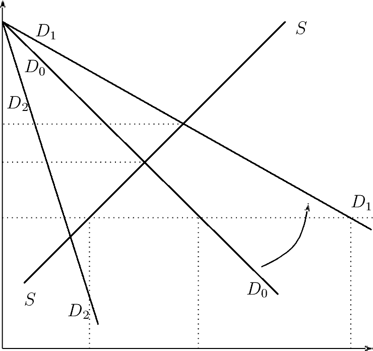
Now that you have seen how market equilibrium can provide benefits to producers and consumers, as measured by producer and consumer surplus, let’s see how taxes affect that surplus. You already know that taxes on suppliers shift the supply curve up. In most cases, equilibrium price (including the tax) rises and equilibrium quantity declines. Taxes on consumers shift the “after-tax” demand curve down, lowering equilibrium quantity and also lowering the price paid to suppliers. But the price demanders pay inclusive of the tax rises (which is why the equilibrium quantity demanded falls). In both cases, taxes reduce, or limit, trade. Economists often talk about the limitations that taxes place on trade as the burden of taxation. Figure 7-2 provides the basic framework for understanding the burden of taxation. For a given good, a per-unit tax $t$ paid by the supplier increases the price at which suppliers are
willing to sell that good. The effect of the tax is shown by a shift upward of the supply curve from $S_0$ to $S_1$. The equilibrium price of the good rises and the quantity sold declines.
Before the tax, consumers pay $P_0$ and producers keep $P_0$. Consumer surplus is represented by areas $A+B+C$, and producer surplus is represented by areas $D+E+$ $F$. With the tax $t$, equilibrium price rises to $P_1$ and equilibrium quantity falls to $Q_1$. Consumers now pay a higher price $P_1$, but producers keep less, only $P_1-t$. Tax revenue paid equals the tax $t$ times equilibrium quantity $Q_1$, or areas $B$ and $D$.
The total cost to consumers and producers is taxes they pay plus lost surplus because of fewer trades. Consumers pay area $B$ in tax revenue and lose area $C$ in consumer surplus. Producers pay area $D$ in tax revenue and lose area $E$ in producer surplus. The triangular area $C+E$ represents a cost of taxation over and above the taxes paid to government. It is lost consumer and producer surplus that is not gained by government. The loss of consumer and producer surplus from a tax is known as deadweight loss. Deadweight loss is shown graphically by the welfare loss triangle- a geometric representation of the welfare cost in terms of misallocated resources caused by a deviation from a supply/demand equilibrium. Keep in mind that with the tax, quantity sold declines. The loss of welfare, therefore, represents a loss for those consumers and producers who, because of the tax, no longer buy or sell goods.
微观经济学代考
经济代写|微观经济学代写Microeconomics代考|Producer and Consumer Surplus
我们通过观察经济学家如何衡量市场对消费者和生产者的好处,开始讨论税收和政府干预的影响;通过考虑供给和需求曲线所告诉我们的,我们可以看到好处。每条曲线都告诉我们个人愿意为一种商品支付多少(在需求情况下)或接受多少(在供给情况下)。因此,在图7-1(a)中,消费者愿意为2单位商品每人支付8美元。供应商愿意以每件2美元的价格出售2件。
如果消费者支付的价格低于他愿意支付的价格,他最终会获得净收益——商品对他的价值减去他为该商品实际支付的价格。因此,需求曲线和他支付的价格之间的距离就是消费者的净收益。经济学家称这种净效益为消费者剩余,即消费者从购买产品中获得的价值减去其价格。它由需求曲线下方和个人支付价格上方的面积表示。因此,当价格处于均衡$($ 5)$时,消费者剩余用蓝色区域表示。
同样,如果生产者得到的价格高于他愿意出售的价格,他也会获得净收益。经济学家称这种收益为生产者剩余——生产者以低于生产成本的价格出售产品。它由供给曲线上方但低于生产者获得的价格的面积表示。因此,当价格处于均衡$($ 5)$时,生产者剩余用棕色区域表示。
市场均衡的好处在于,它使消费者和生产者的剩余组合尽可能大。为了理解这一点,假设由于某种原因,均衡价格保持在$\$ 6$。消费者将只需要4单位的商品,一些供应商无法销售他们想要的所有商品。生产者剩余和消费者剩余的总和将减少,如图7-1(b)所示。灰色三角形代表失去的消费者和生产者剩余。一般来说,价格偏离均衡会降低生产者和消费者剩余的总和。这是经济学家支持市场的原因之一,也是我们教授供求模型的原因之一。它让我们直观地感受到市场的好处:通过允许贸易,市场最大化了消费者和生产者剩余的组合。
对于直线需求曲线,剩余量可以通过计算相关三角形或矩形的面积来确定。例如,在图7-1(a)中,消费者剩余三角形的底为5,高为5(10-5)。因为三角形的面积是$1 / $ 2(底$ $\乘以高$ $),所以消费者剩余是12.5单位。或者,在图7-1(b)中,高于均衡价格的价格损失的剩余为1。这是通过确定三角形的高度(从侧面看)是$1(5-4)$和底面是$2(6-4)$来计算的,使得损失的剩余面积$1 / 2 \乘以2 \乘以1=1$。在这种情况下,消费者和生产者平均分担损失。较高的价格将4个单位的剩余从消费者转移到生产者,计算方法是确定由原点和产出4以及价格5和6形成的矩形的面积(底乘以高),这等于(6-5)乘以(4-0)=4美元。这就给消费者留下了8单位剩余。${} ^ 1美元
为了在你的脑海中固定消费者和生产者剩余的概念,让我们考虑几个现实世界的例子。想想你喝的水。它的价格是多少?几乎没有。考虑到水很容易获得,它的价格很低。但是如果你没有水,你会渴死的,你从这些水中获得了大量的消费者剩余。接下来,考虑一个非常喜欢芭蕾舞的芭蕾舞者,他愿意免费跳舞。但他发现人们愿意花钱看他演出,而他一场演出可以得到4000美元。他得到了生产者剩余。
经济代写|微观经济学代写Microeconomics代考|Burden of Taxation
既然你已经了解了市场均衡如何通过生产者和消费者剩余来为生产者和消费者提供利益,那么让我们看看税收是如何影响生产者和消费者剩余的。你们已经知道,对供应商征税会使供给曲线上移。在大多数情况下,均衡价格(包括税收)上升,均衡数量下降。对消费者征税使“税后”需求曲线下移,降低了均衡量,也降低了支付给供应商的价格。但是需求者支付的价格包含了税收的增加(这就是均衡需求量下降的原因)。在这两种情况下,税收都会减少或限制贸易。经济学家经常把税收对贸易的限制称为税收负担。图7-2提供了了解税收负担的基本框架。对于给定商品,供应商支付的每单位税增加了供应商的价格
愿意卖那个好东西。税收的影响表现为供给曲线从$S_0$向上移动到$S_1$。商品的均衡价格上升,销售量下降。
在征税之前,消费者支付$P_0$,生产者保留$P_0$。消费者剩余由区域$A+B+C$表示,生产者剩余由区域$D+E+$ F$表示。当税$t$时,均衡价格上升到$P_1$,均衡数量下降到$Q_1$。消费者现在支付更高的价格$P_1$,但生产者保留的更少,只有$P_1$ t$。支付的税收等于税收t乘以均衡量Q_1,或者面积B和D。
消费者和生产者的总成本是他们支付的税收加上由于贸易减少而损失的盈余。消费者支付区域B$的税收,损失区域C$的消费者剩余。生产者支付区域D$的税收,而损失区域E$的生产者剩余。三角形区域C+E表示在支付给政府的税收之外的税收成本。政府没有得到的是消费者和生产者剩余的损失。消费者和生产者剩余的税收损失被称为无谓损失。无谓损失由福利损失三角形图形表示——福利成本的几何表示,以偏离供需平衡导致的资源分配不当为依据。请记住,随着税收的增加,销售量会下降。因此,福利的损失对那些由于税收而不再买卖商品的消费者和生产者来说是一种损失。

统计代写请认准statistics-lab™. statistics-lab™为您的留学生涯保驾护航。
金融工程代写
金融工程是使用数学技术来解决金融问题。金融工程使用计算机科学、统计学、经济学和应用数学领域的工具和知识来解决当前的金融问题,以及设计新的和创新的金融产品。
非参数统计代写
非参数统计指的是一种统计方法,其中不假设数据来自于由少数参数决定的规定模型;这种模型的例子包括正态分布模型和线性回归模型。
广义线性模型代考
广义线性模型(GLM)归属统计学领域,是一种应用灵活的线性回归模型。该模型允许因变量的偏差分布有除了正态分布之外的其它分布。
术语 广义线性模型(GLM)通常是指给定连续和/或分类预测因素的连续响应变量的常规线性回归模型。它包括多元线性回归,以及方差分析和方差分析(仅含固定效应)。
有限元方法代写
有限元方法(FEM)是一种流行的方法,用于数值解决工程和数学建模中出现的微分方程。典型的问题领域包括结构分析、传热、流体流动、质量运输和电磁势等传统领域。
有限元是一种通用的数值方法,用于解决两个或三个空间变量的偏微分方程(即一些边界值问题)。为了解决一个问题,有限元将一个大系统细分为更小、更简单的部分,称为有限元。这是通过在空间维度上的特定空间离散化来实现的,它是通过构建对象的网格来实现的:用于求解的数值域,它有有限数量的点。边界值问题的有限元方法表述最终导致一个代数方程组。该方法在域上对未知函数进行逼近。[1] 然后将模拟这些有限元的简单方程组合成一个更大的方程系统,以模拟整个问题。然后,有限元通过变化微积分使相关的误差函数最小化来逼近一个解决方案。
tatistics-lab作为专业的留学生服务机构,多年来已为美国、英国、加拿大、澳洲等留学热门地的学生提供专业的学术服务,包括但不限于Essay代写,Assignment代写,Dissertation代写,Report代写,小组作业代写,Proposal代写,Paper代写,Presentation代写,计算机作业代写,论文修改和润色,网课代做,exam代考等等。写作范围涵盖高中,本科,研究生等海外留学全阶段,辐射金融,经济学,会计学,审计学,管理学等全球99%专业科目。写作团队既有专业英语母语作者,也有海外名校硕博留学生,每位写作老师都拥有过硬的语言能力,专业的学科背景和学术写作经验。我们承诺100%原创,100%专业,100%准时,100%满意。
随机分析代写
随机微积分是数学的一个分支,对随机过程进行操作。它允许为随机过程的积分定义一个关于随机过程的一致的积分理论。这个领域是由日本数学家伊藤清在第二次世界大战期间创建并开始的。
时间序列分析代写
随机过程,是依赖于参数的一组随机变量的全体,参数通常是时间。 随机变量是随机现象的数量表现,其时间序列是一组按照时间发生先后顺序进行排列的数据点序列。通常一组时间序列的时间间隔为一恒定值(如1秒,5分钟,12小时,7天,1年),因此时间序列可以作为离散时间数据进行分析处理。研究时间序列数据的意义在于现实中,往往需要研究某个事物其随时间发展变化的规律。这就需要通过研究该事物过去发展的历史记录,以得到其自身发展的规律。
回归分析代写
多元回归分析渐进(Multiple Regression Analysis Asymptotics)属于计量经济学领域,主要是一种数学上的统计分析方法,可以分析复杂情况下各影响因素的数学关系,在自然科学、社会和经济学等多个领域内应用广泛。
MATLAB代写
MATLAB 是一种用于技术计算的高性能语言。它将计算、可视化和编程集成在一个易于使用的环境中,其中问题和解决方案以熟悉的数学符号表示。典型用途包括:数学和计算算法开发建模、仿真和原型制作数据分析、探索和可视化科学和工程图形应用程序开发,包括图形用户界面构建MATLAB 是一个交互式系统,其基本数据元素是一个不需要维度的数组。这使您可以解决许多技术计算问题,尤其是那些具有矩阵和向量公式的问题,而只需用 C 或 Fortran 等标量非交互式语言编写程序所需的时间的一小部分。MATLAB 名称代表矩阵实验室。MATLAB 最初的编写目的是提供对由 LINPACK 和 EISPACK 项目开发的矩阵软件的轻松访问,这两个项目共同代表了矩阵计算软件的最新技术。MATLAB 经过多年的发展,得到了许多用户的投入。在大学环境中,它是数学、工程和科学入门和高级课程的标准教学工具。在工业领域,MATLAB 是高效研究、开发和分析的首选工具。MATLAB 具有一系列称为工具箱的特定于应用程序的解决方案。对于大多数 MATLAB 用户来说非常重要,工具箱允许您学习和应用专业技术。工具箱是 MATLAB 函数(M 文件)的综合集合,可扩展 MATLAB 环境以解决特定类别的问题。可用工具箱的领域包括信号处理、控制系统、神经网络、模糊逻辑、小波、仿真等。