
如果你也在 怎样代写多元统计分析Multivariate Statistical Analysis这个学科遇到相关的难题,请随时右上角联系我们的24/7代写客服。
多元统计分析Multivariate Statistical Analysis是基于多变量统计的原理。通常情况下,MVA用于解决对每个实验单元进行多次测量的情况,这些测量之间的关系及其结构很重要。现代的、重叠的MVA分类包括:正态和一般多变量模型和分布理论、关系的研究和测量、多维区域的概率计算、对数据结构和模式的探索、由于希望包括基于物理学的分析,以计算变量对分层 “系统中的系统 “的影响,多变量分析可能变得复杂。通常情况下,希望使用多变量分析的研究会因为问题的维度而停滞。这些问题通常通过使用代理模型来缓解,代理模型是基于物理学的代码的高度精确的近似。由于代用模型采取方程的形式,它们可以被快速评估。这成为大规模MVA研究的一个有利因素:在基于物理学的代码中,整个设计空间的蒙特卡洛模拟是困难的,而在评估代用模型时,它变得微不足道,代用模型通常采取响应面方程式的形式。
statistics-lab™ 为您的留学生涯保驾护航 在代写多元统计分析Multivariate Statistical Analysis方面已经树立了自己的口碑, 保证靠谱, 高质且原创的统计Statistics代写服务。我们的专家在代写多元统计分析Multivariate Statistical Analysis代写方面经验极为丰富,各种代写多元统计分析Multivariate Statistical Analysis相关的作业也就用不着说。
统计代写|多元统计分析代写Multivariate Statistical Analysis代考|Aim of the Analysis
The Boston Housing data set was analyzed by Harrison and Rubinfeld (1978) who wanted to find out whether “clean air” had an influence on house prices. We will use this data set in this chapter and in most of the following chapters to illustrate the presented methodology. The data are described in Appendix B.1.
What Can Be Seen from the PCPs
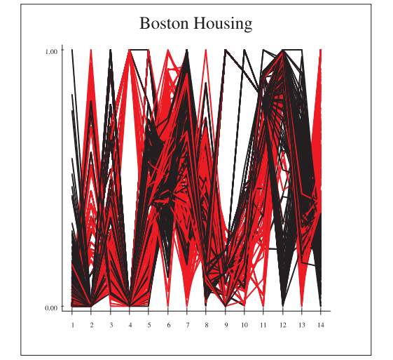
In order to highlight the relations of $X_{14}$ to the remaining 13 variables we color all of the observations with $X_{14}>$ median $\left(X_{14}\right)$ as red lines in Figure 1.24. Some of the variables seem to be strongly related. The most obvious relation is the negative dependence between $X_{13}$ and $X_{14}$. It can also be argued that there exists a strong dependence between $X_{12}$ and $X_{14}$ since no red lines are drawn in the lower part of $X_{12}$. The opposite can be said about $X_{11}$ : there are only red lines plotted in the lower part of this variable. Low values of $X_{11}$ induce high values of $X_{14}$.
For the PCP, the variables have been rescaled over the interval $[0,1]$ for better graphical representations. The $\mathrm{PCP}$ shows that the variables are not distributed in a symmetric manner. It can be clearly seen that the values of $X_1$ and $X_9$ are much more concentrated around 0 . Therefore it makes sense to consider transformations of the original data.
The Scatterplot Matrix
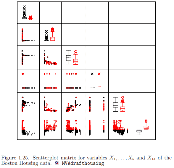
One characteristic of the PCPs is that many lines are drawn on top of each other. This problem is reduced by depicting the variables in pairs of scatterplots. Including all 14 variables in one large scatterplot matrix is possible, but makes it hard to see anything from the plots. Therefore, for illustratory purposes we will analyze only one such matrix from a subset of the variables in Figure 1.25. On the basis of the PCP and the scatterplot matrix we would like to interpret each of the thirteen variables and their eventual relation to the 14th variable. Included in the figure are images for $X_1-X_5$ and $X_{14}$, although each variable is discussed in detail below. All references made to scatterplots in the following refer to Figure 1.25.
统计代写|多元统计分析代写Multivariate Statistical Analysis代考|Per-capita crime rate X1
Taking the logarithm makes the variable’s distribution more symmetric. This can be seen in the boxplot of $\widetilde{X}1$ in Figure 1.27 which shows that the median and the mean have moved closer to each other than they were for the original $X_1$. Plotting the kernel density estimate (KDE) of $\widetilde{X}_1=\log \left(X_1\right)$ would reveal that two subgroups might exist with different mean values. However, taking a look at the scatterplots in Figure 1.26 of the logarithms which include $X_1$ does not clearly reveal such groups. Given that the scatterplot of $\log \left(X_1\right)$ vs. $\log \left(X{14}\right)$ shows a relatively strong negative relation, it might be the case that the two subgroups of $X_1$ correspond to houses with two different price levels. This is confirmed by the two boxplots shown to the right of the $X_1$ vs. $X_2$ scatterplot (in Figure 1.25): the right boxplot’s shape differs a lot from the black one’s, having a much higher median and mean.
Proportion of residential area zoned for large lots $X_2$
It strikes the eye in Figure 1.25 that there is a large cluster of observations for which $X_2$ is equal to 0 . It also strikes the eye that-as the scatterplot of $X_1$ vs. $X_2$ shows-there is a strong, though non-linear, negative relation between $X_1$ and $X_2$ : Almost all observations for which $X_2$ is high have an $X_1$-value close to zero, and vice versa, many observations for which $X_2$ is zero have quite a high per-capita crime rate $X_1$. This could be due to the location of the areas, e.g., downtown districts might have a higher crime rate and at the same time it is unlikely that any residential land would be zoned in a generous manner.
As far as the house prices are concerned it can be said that there seems to be no clear (linear) relation between $X_2$ and $X_{14}$, but it is obvious that the more expensive houses are situated in areas where $X_2$ is large (this can be seen from the two boxplots on the second position of the diagonal, where the red one has a clearly higher mean/median than the black one).
多元统计分析代考
统计代写|多元统计分析代写Multivariate Statistical Analysis代考|Aim of the Analysis
Harrison和Rubinfeld(1978)分析了Boston Housing的数据集,他们想要找出“清洁空气”是否对房价有影响。我们将在本章和接下来的大部分章节中使用这个数据集来说明所提出的方法。数据见附录B.1。
从pcp可以看到什么
为了突出$X_{14}$与其余13个变量的关系,我们将图1.24中位数为$X_{14}>$$\left(X_{14}\right)$的所有观测值涂成红线。其中一些变量似乎密切相关。最明显的关系是$X_{13}$和$X_{14}$之间的负相关关系。也可以认为$X_{12}$和$X_{14}$之间存在很强的依赖性,因为$X_{12}$的下半部分没有画红线。$X_{11}$的情况正好相反:在这个变量的下半部分只有红线。低的$X_{11}$值会导致高的$X_{14}$值。
对于PCP,变量已经在$[0,1]$区间内重新缩放,以获得更好的图形表示。$\mathrm{PCP}$显示变量不是对称分布的。可以清楚地看到,$X_1$和$X_9$的值更加集中在0附近。因此,考虑原始数据的转换是有意义的。
散点图矩阵
pcp的一个特点是,许多线被画在彼此的顶部。用成对的散点图来描述变量可以减少这个问题。在一个大的散点图矩阵中包含所有14个变量是可能的,但很难从图中看到任何东西。因此,为了便于说明,我们将只分析图1.25中变量子集中的一个这样的矩阵。在PCP和散点图矩阵的基础上,我们想解释13个变量中的每一个以及它们与第14个变量的最终关系。图中包括$X_1-X_5$和$X_{14}$的图像,下面将详细讨论每个变量。下面对散点图的所有引用参见图1.25。
统计代写|多元统计分析代写Multivariate Statistical Analysis代考|Per-capita crime rate X1
取对数使变量的分布更加对称。这可以从图1.27中$\widetilde{X}1$的箱线图中看到,该箱线图显示中位数和平均值比原始$X_1$更接近彼此。绘制$\widetilde{X}1=\log \left(X_1\right)$的核密度估计(KDE)将揭示可能存在两个具有不同平均值的子组。然而,看一看图1.26中包含$X_1$的对数的散点图,并没有清楚地揭示出这样的群体。鉴于$\log \left(X_1\right)$与$\log \left(X{14}\right)$的散点图显示出相对较强的负相关,$X_1$的两个子组可能对应于两个不同价格水平的房屋。这一点在$X_1$与$X_2$散点图右侧的两个箱形图中得到了证实(见图1.25):右侧箱形图的形状与黑色箱形图的形状有很大不同,中间值和平均值都要高得多。 划分为大型地块的住宅面积比例$X_2$ 在图1.25中可以看到,有一大簇观测值,其中$X_2$等于0。同样引人注目的是,正如$X_1$与$X_2$的散点图所显示的那样,$X_1$和$X_2$之间存在着一种强烈的,尽管是非线性的负相关关系:几乎所有的观测值中,$X_2$值高的$X_1$值都接近于零,反之亦然,许多观测值中$X_2$值为零的人均犯罪率都相当高$X_1$。这可能是由于这些地区的地理位置,例如,市中心地区可能有较高的犯罪率,同时,任何住宅用地都不太可能以慷慨的方式分区。 就房价而言,可以说$X_2$和$X{14}$之间似乎没有明确的(线性)关系,但很明显,更昂贵的房子位于$X_2$较大的地区(这可以从对角线第二个位置的两个箱形图中看出,其中红色的平均值/中位数明显高于黑色的)。

统计代写请认准statistics-lab™. statistics-lab™为您的留学生涯保驾护航。
金融工程代写
金融工程是使用数学技术来解决金融问题。金融工程使用计算机科学、统计学、经济学和应用数学领域的工具和知识来解决当前的金融问题,以及设计新的和创新的金融产品。
非参数统计代写
非参数统计指的是一种统计方法,其中不假设数据来自于由少数参数决定的规定模型;这种模型的例子包括正态分布模型和线性回归模型。
广义线性模型代考
广义线性模型(GLM)归属统计学领域,是一种应用灵活的线性回归模型。该模型允许因变量的偏差分布有除了正态分布之外的其它分布。
术语 广义线性模型(GLM)通常是指给定连续和/或分类预测因素的连续响应变量的常规线性回归模型。它包括多元线性回归,以及方差分析和方差分析(仅含固定效应)。
有限元方法代写
有限元方法(FEM)是一种流行的方法,用于数值解决工程和数学建模中出现的微分方程。典型的问题领域包括结构分析、传热、流体流动、质量运输和电磁势等传统领域。
有限元是一种通用的数值方法,用于解决两个或三个空间变量的偏微分方程(即一些边界值问题)。为了解决一个问题,有限元将一个大系统细分为更小、更简单的部分,称为有限元。这是通过在空间维度上的特定空间离散化来实现的,它是通过构建对象的网格来实现的:用于求解的数值域,它有有限数量的点。边界值问题的有限元方法表述最终导致一个代数方程组。该方法在域上对未知函数进行逼近。[1] 然后将模拟这些有限元的简单方程组合成一个更大的方程系统,以模拟整个问题。然后,有限元通过变化微积分使相关的误差函数最小化来逼近一个解决方案。
tatistics-lab作为专业的留学生服务机构,多年来已为美国、英国、加拿大、澳洲等留学热门地的学生提供专业的学术服务,包括但不限于Essay代写,Assignment代写,Dissertation代写,Report代写,小组作业代写,Proposal代写,Paper代写,Presentation代写,计算机作业代写,论文修改和润色,网课代做,exam代考等等。写作范围涵盖高中,本科,研究生等海外留学全阶段,辐射金融,经济学,会计学,审计学,管理学等全球99%专业科目。写作团队既有专业英语母语作者,也有海外名校硕博留学生,每位写作老师都拥有过硬的语言能力,专业的学科背景和学术写作经验。我们承诺100%原创,100%专业,100%准时,100%满意。
随机分析代写
随机微积分是数学的一个分支,对随机过程进行操作。它允许为随机过程的积分定义一个关于随机过程的一致的积分理论。这个领域是由日本数学家伊藤清在第二次世界大战期间创建并开始的。
时间序列分析代写
随机过程,是依赖于参数的一组随机变量的全体,参数通常是时间。 随机变量是随机现象的数量表现,其时间序列是一组按照时间发生先后顺序进行排列的数据点序列。通常一组时间序列的时间间隔为一恒定值(如1秒,5分钟,12小时,7天,1年),因此时间序列可以作为离散时间数据进行分析处理。研究时间序列数据的意义在于现实中,往往需要研究某个事物其随时间发展变化的规律。这就需要通过研究该事物过去发展的历史记录,以得到其自身发展的规律。
回归分析代写
多元回归分析渐进(Multiple Regression Analysis Asymptotics)属于计量经济学领域,主要是一种数学上的统计分析方法,可以分析复杂情况下各影响因素的数学关系,在自然科学、社会和经济学等多个领域内应用广泛。
MATLAB代写
MATLAB 是一种用于技术计算的高性能语言。它将计算、可视化和编程集成在一个易于使用的环境中,其中问题和解决方案以熟悉的数学符号表示。典型用途包括:数学和计算算法开发建模、仿真和原型制作数据分析、探索和可视化科学和工程图形应用程序开发,包括图形用户界面构建MATLAB 是一个交互式系统,其基本数据元素是一个不需要维度的数组。这使您可以解决许多技术计算问题,尤其是那些具有矩阵和向量公式的问题,而只需用 C 或 Fortran 等标量非交互式语言编写程序所需的时间的一小部分。MATLAB 名称代表矩阵实验室。MATLAB 最初的编写目的是提供对由 LINPACK 和 EISPACK 项目开发的矩阵软件的轻松访问,这两个项目共同代表了矩阵计算软件的最新技术。MATLAB 经过多年的发展,得到了许多用户的投入。在大学环境中,它是数学、工程和科学入门和高级课程的标准教学工具。在工业领域,MATLAB 是高效研究、开发和分析的首选工具。MATLAB 具有一系列称为工具箱的特定于应用程序的解决方案。对于大多数 MATLAB 用户来说非常重要,工具箱允许您学习和应用专业技术。工具箱是 MATLAB 函数(M 文件)的综合集合,可扩展 MATLAB 环境以解决特定类别的问题。可用工具箱的领域包括信号处理、控制系统、神经网络、模糊逻辑、小波、仿真等。