如果你也在 怎样代写网络分析Network Analysis这个学科遇到相关的难题,请随时右上角联系我们的24/7代写客服。
网络分析研究实体之间的关系,如个人、组织或文件。在多个层面上操作,它描述并推断单个实体、实体的子集和整个网络的关系属性。
statistics-lab™ 为您的留学生涯保驾护航 在代写网络分析Network Analysis方面已经树立了自己的口碑, 保证靠谱, 高质且原创的统计Statistics代写服务。我们的专家在代写网络分析Network Analysis代写方面经验极为丰富,各种代写网络分析Network Analysis相关的作业也就用不着说。
我们提供的网络分析Network Analysis及其相关学科的代写,服务范围广, 其中包括但不限于:
- Statistical Inference 统计推断
- Statistical Computing 统计计算
- Advanced Probability Theory 高等概率论
- Advanced Mathematical Statistics 高等数理统计学
- (Generalized) Linear Models 广义线性模型
- Statistical Machine Learning 统计机器学习
- Longitudinal Data Analysis 纵向数据分析
- Foundations of Data Science 数据科学基础
统计代写|网络分析代写Network Analysis代考|Basic concepts
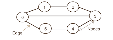
A graph [3] is a pictorial representation of a set of objects and their association with each other. The objects are popularly termed as nodes or vertices, and the associations are depicted using interconnections between pair of nodes, called edges. Mathematically, graphs are represented as a set of edges and vertices.
Definition 2.1.1 (Graph). A graph $\mathcal{G}$ is a pair of finite set of vertices and edges, $\mathcal{G}=(\mathcal{V}, \mathcal{E})$, such that $\mathcal{V}=\left{v_1, v_2, \cdots, v_n\right}$ and $\mathcal{E}=$ $\left{e_1, e_2, \cdots, e_m\right}$. An edge $e_k=\left(v_i, v_j\right)$ connects vertices $v_i$ and $v_j$.
In the graph (Fig. 2.1), $\mathcal{V}={A, B, C, D, E, F}$ and $\mathcal{E}={(A, B)$, $(B, C),(C, D),(C, E),(E, E),(E, F),(E, D),(F, B)}$, where edges are an unordered pair of nodes having interconnections among them. Graph $\mathcal{G}$ is termed as undirected graph. The node $E$ is connected with itself through loop edge. A graph without my loop structure is called a simple graph.
A graph with an ordered pair of nodes, where edges are associated with directions is called a directed graph or digraph.
Definition 2.1.2 (Directed graph). A directed graph $\mathcal{G}=(\mathcal{V}, \mathcal{E}$ ) is a set of vertices $\mathcal{V}$ and edges $\mathcal{E}$, such that, for any edge $\left(v_i, v_j\right)$ posses direction denoted by arrow. Unlike undirected graph, for any edge $v_i \rightarrow v_j$, the edge $\left(v_i, v_j\right) \neq\left(v_j, v_i\right)$. The node $v_i$ is called tail, and $v_j$ is referred to as head of the edge $v_i \rightarrow v_j$. For example, see Fig. 2.2.
Definition 2.1.3 (Path). A path is a sequence of distinct vertices that are connected by edges. In other words, given a set of vertices, $\left{v_1, v_2, \cdots, v_k\right} \in \mathcal{G}(\mathcal{V})$ is a path if for every pair of vertices $v_i$ and $v_{i+1}$ have an edge $\left(v_i, v_{i+1}\right) \in \mathcal{G}(\mathcal{E})$. However, in case of a directed graph, a directed path connects the sequence of vertices with the added restriction that all edges are oriented towards the same direction.
In a path, if sequences of vertices are not distinct, it is referred to as a walk.
Two nodes, $v_i$ and $v_j$, are reachable from each other if there is a path that exists between $v_i$ and $v_j$.
A path is called a closed path or cycle if two terminal nodes, $v_1$ and $v_k$, are connected in a path, i.e., $\left(v_k, v_1\right) \in \mathcal{G}(\mathcal{E})$.
In Fig. 2.1, $A-B-C-D$ or $A-B-F-E$ are two different paths, whereas $A \rightarrow B \rightarrow C \rightarrow D$ is a directed path existing in the directed graph (Fig. 2.2), but path $A \rightarrow B \rightarrow F \rightarrow E$ does not exist.
统计代写|网络分析代写Network Analysis代考|Data structure for representing graphs
The sequential representation of a graph using an array data structure uses a two-dimensional array or matrix called adjacency matrix.
Definition 2.2.1 (Adjacency matrix). Given a graph $\mathcal{G}=(\mathcal{V}, \mathcal{E}$ ), an adjacency matrix, say $A d j$ is a square matrix of size $|\mathcal{V}| \times|\mathcal{V}|$. Each cell of Adj indicates an edge between any two vertices or nodes:
$$
A d j[i][j]=\left{\begin{array}{cl}
\omega, & \text { if }\left(v_i, v_j\right) \in \mathcal{G}(\mathcal{E}) \
0, & \text { otherwise, }
\end{array}\right.
$$
where $\omega$ is the weight of the edge between the nodes $v_i$ and $v_j$. In the case of an unweighted graph, $\omega$ is considered as 1 , whereas for weighted graph it may be any value according to the problem in hand. See Fig. 2.10.
Adjacency matrices of undirected graphs are symmetric, where $A d j[i][j]=A d j[j][i]$, for $i, j$. In other words, we may say that $A d j$ and its transpose Adj’ is the same. Unlike undirected graph, digraph produces asymmetric matrix.
Finding degree of a node
One of the important operations on a graph is finding the degree of a given node. From the adjacency matrix, it is easy to determine the connection of any nodes. The degree of a node in an undirected graph can be calculated as follows:
$$
\operatorname{deg}\left(v_i\right)=\sum_{j=1}^n \operatorname{Adj}[i][j]
$$ where values in the $i^{t h}$ row in the adjacency matrix indicates the connections to $n$ different nodes from the node $i$ in the graph. Similarly, in the case of digraph, the indegree and outdegree of a node can be calculated as follows:
$$
\text { indeg }\left(v_i\right)=\sum_{j=1}^n \operatorname{Adj}[j][i] \text { and outdeg }\left(v_i\right)=\sum_{j=1}^n \operatorname{Adj}[i][j] \text {. }
$$
网络分析代考
统计代写|网络分析代写Network Analysis代考|Basic concepts
图 [3] 是一组对象及其相互关联的图形表示。这些对象通常称为节点或顶点,并且使用一对节点(称为 边) 之间的互连来描述关联。在数学上,图表示为一组边和顶点。
定义 2.1 .1 (图表)。一张图 $\mathcal{G}$ 是一对有限的顶点和边集, $\mathcal{G}=(\mathcal{V}, \mathcal{E})$ , 这样 $e_k=\left(v_i, v_j\right)$ 连接顶点 $v_i$ 和 $v_j$.
在图中 (图 2.1), $\mathcal{V}=A, B, C, D, E, F$ 和
$\mathcal{E}=(A, B) \$, \$(B, C),(C, D),(C, E),(E, E),(E, F),(E, D),(F, B)$ ,其中边是一对无序的 节点,它们之间有互连。图形 $\mathcal{G}$ 被称为无向图。节点 $E$ 通过循环边与自身相连。没有我的循环结构的图 称为简单图。
具有一对有序节点的图,其中边与方向相关联,称为有向图或有向图。
定义 2.1 .2 (有向图) 。有向图 $\mathcal{G}=(\mathcal{V}, \mathcal{E})$ 是一组顶点 $\mathcal{V}$ 和边缘 $\mathcal{E}$ ,这样,对于任何边缘 $\left(v_i, v_j\right)$ 具有箭 头指示的方向。与无向图不同,对于任意边 $v_i \rightarrow v_j$ ,边缘 $\left(v_i, v_j\right) \neq\left(v_j, v_i\right)$. 节点 $v_i$ 称为尾巴,并 且 $v_j$ 被称为边缘的头部 $v_i \rightarrow v_j$. 例如,见图 2.2。
定义 2.1.3 (路径) 。路径是由边连接的不同顶点序列。换句话说,给定一组顶点, 优势 $\left(v_i, v_{i+1}\right) \in \mathcal{G}(\mathcal{E})$. 然而,在有向图的情况下,有向路径连接顶点序列,并添加了所有边都朝向相 同方向的限制。
在一条路径中,如果顶点序列不明显,则称为行走。
两个节点, $v_i$ 和 $v_j$ ,如果之间存在一条路径,则彼此可达 $v_i$ 和 $v_j$.
如果有两个终端节点,则路径称为闭合路径或循环, $v_1$ 和 $v_k$ ,连接在一条路径上,即 $\left(v_k, v_1\right) \in \mathcal{G}(\mathcal{E})$.
在图 2.1 中, $A-B-C-D$ 或者 $A-B-F-E$ 是两条不同的路径,而 $A \rightarrow B \rightarrow C \rightarrow D$ 是 有向图中存在的有向路径 (图2.2),但路径 $A \rightarrow B \rightarrow F \rightarrow E$ 不存在。
统计代写|网络分析代写Network Analysis代考|Data structure for representing graphs
使用数组数据结构的图的顺序表示使用称为邻接矩阵的二维数组或矩阵。
定义 2.2.1 (邻接矩阵) 。给定一个图 $\mathcal{G}=(\mathcal{V}, \mathcal{E}$ ),一个邻接矩阵, 比如 $A d j$ 是大小的方阵 $|\mathcal{V}| \times|\mathcal{V}|$. Adj 的每个单元表示任意两个顶点或节点之间的一条边: $\$ \$$
A dj $[i][j]=\backslash l e f t{$
$\omega, \quad$ if $\left(v_i, v_j\right) \in \mathcal{G}(\mathcal{E}) 0, \quad$ otherwise,
、止确的。 $\$ \$$
哪里 $\omega$ 是节点之间边的权重 $v_i$ 和 $v_j$. 在末加权图的情况下, $\omega$ 被认为是 1 ,而对于加权图,它可以是根据 手头问题的任何值。见图 2.10。
无向图的邻接矩阵是对称的,其中 $A d j[i][j]=A d j[j][i]$ ,为了 $i, j$. 换句话说,我们可以说 $A d j$ 并且 它的转置 Adj’ 是相同的。与无向图不同,有向图产生非对称矩阵。
查找节点的廂
图的重要操作之一是查找给定节点的度。从邻接矩阵中,很容易确定任意节点的连接。无向图中节点的 度可以计算如下:
$$
\operatorname{deg}\left(v_i\right)=\sum_{j=1}^n \operatorname{Adj}[i][j]
$$
其中值在 $i^{t h}$ 邻接矩阵中的行表示与 $n$ 来自节点的不同节点 $i$ 在图中。同样,在有向图的情况下,节点的入 度和出度可以计算如下:
$$
\operatorname{indeg}\left(v_i\right)=\sum_{j=1}^n \operatorname{Adj}[j][i] \text { and outdeg }\left(v_i\right)=\sum_{j=1}^n \operatorname{Adj}[i][j] .
$$

统计代写请认准statistics-lab™. statistics-lab™为您的留学生涯保驾护航。
金融工程代写
金融工程是使用数学技术来解决金融问题。金融工程使用计算机科学、统计学、经济学和应用数学领域的工具和知识来解决当前的金融问题,以及设计新的和创新的金融产品。
非参数统计代写
非参数统计指的是一种统计方法,其中不假设数据来自于由少数参数决定的规定模型;这种模型的例子包括正态分布模型和线性回归模型。
广义线性模型代考
广义线性模型(GLM)归属统计学领域,是一种应用灵活的线性回归模型。该模型允许因变量的偏差分布有除了正态分布之外的其它分布。
术语 广义线性模型(GLM)通常是指给定连续和/或分类预测因素的连续响应变量的常规线性回归模型。它包括多元线性回归,以及方差分析和方差分析(仅含固定效应)。
有限元方法代写
有限元方法(FEM)是一种流行的方法,用于数值解决工程和数学建模中出现的微分方程。典型的问题领域包括结构分析、传热、流体流动、质量运输和电磁势等传统领域。
有限元是一种通用的数值方法,用于解决两个或三个空间变量的偏微分方程(即一些边界值问题)。为了解决一个问题,有限元将一个大系统细分为更小、更简单的部分,称为有限元。这是通过在空间维度上的特定空间离散化来实现的,它是通过构建对象的网格来实现的:用于求解的数值域,它有有限数量的点。边界值问题的有限元方法表述最终导致一个代数方程组。该方法在域上对未知函数进行逼近。[1] 然后将模拟这些有限元的简单方程组合成一个更大的方程系统,以模拟整个问题。然后,有限元通过变化微积分使相关的误差函数最小化来逼近一个解决方案。
tatistics-lab作为专业的留学生服务机构,多年来已为美国、英国、加拿大、澳洲等留学热门地的学生提供专业的学术服务,包括但不限于Essay代写,Assignment代写,Dissertation代写,Report代写,小组作业代写,Proposal代写,Paper代写,Presentation代写,计算机作业代写,论文修改和润色,网课代做,exam代考等等。写作范围涵盖高中,本科,研究生等海外留学全阶段,辐射金融,经济学,会计学,审计学,管理学等全球99%专业科目。写作团队既有专业英语母语作者,也有海外名校硕博留学生,每位写作老师都拥有过硬的语言能力,专业的学科背景和学术写作经验。我们承诺100%原创,100%专业,100%准时,100%满意。
随机分析代写
随机微积分是数学的一个分支,对随机过程进行操作。它允许为随机过程的积分定义一个关于随机过程的一致的积分理论。这个领域是由日本数学家伊藤清在第二次世界大战期间创建并开始的。
时间序列分析代写
随机过程,是依赖于参数的一组随机变量的全体,参数通常是时间。 随机变量是随机现象的数量表现,其时间序列是一组按照时间发生先后顺序进行排列的数据点序列。通常一组时间序列的时间间隔为一恒定值(如1秒,5分钟,12小时,7天,1年),因此时间序列可以作为离散时间数据进行分析处理。研究时间序列数据的意义在于现实中,往往需要研究某个事物其随时间发展变化的规律。这就需要通过研究该事物过去发展的历史记录,以得到其自身发展的规律。
回归分析代写
多元回归分析渐进(Multiple Regression Analysis Asymptotics)属于计量经济学领域,主要是一种数学上的统计分析方法,可以分析复杂情况下各影响因素的数学关系,在自然科学、社会和经济学等多个领域内应用广泛。
MATLAB代写
MATLAB 是一种用于技术计算的高性能语言。它将计算、可视化和编程集成在一个易于使用的环境中,其中问题和解决方案以熟悉的数学符号表示。典型用途包括:数学和计算算法开发建模、仿真和原型制作数据分析、探索和可视化科学和工程图形应用程序开发,包括图形用户界面构建MATLAB 是一个交互式系统,其基本数据元素是一个不需要维度的数组。这使您可以解决许多技术计算问题,尤其是那些具有矩阵和向量公式的问题,而只需用 C 或 Fortran 等标量非交互式语言编写程序所需的时间的一小部分。MATLAB 名称代表矩阵实验室。MATLAB 最初的编写目的是提供对由 LINPACK 和 EISPACK 项目开发的矩阵软件的轻松访问,这两个项目共同代表了矩阵计算软件的最新技术。MATLAB 经过多年的发展,得到了许多用户的投入。在大学环境中,它是数学、工程和科学入门和高级课程的标准教学工具。在工业领域,MATLAB 是高效研究、开发和分析的首选工具。MATLAB 具有一系列称为工具箱的特定于应用程序的解决方案。对于大多数 MATLAB 用户来说非常重要,工具箱允许您学习和应用专业技术。工具箱是 MATLAB 函数(M 文件)的综合集合,可扩展 MATLAB 环境以解决特定类别的问题。可用工具箱的领域包括信号处理、控制系统、神经网络、模糊逻辑、小波、仿真等。