标签: CS224W

计算机代写|神经网络代写neural networks代考|CS224W

如果你也在 怎样代写神经网络neural networks这个学科遇到相关的难题,请随时右上角联系我们的24/7代写客服。

神经网络,也被称为人工神经网络(ANN)或模拟神经网络(SNN),是机器学习的一个子集,是深度学习算法的核心。它们的名称和结构受到人脑的启发,模仿了生物神经元相互之间的信号方式。

statistics-lab™ 为您的留学生涯保驾护航 在代写神经网络neural networks方面已经树立了自己的口碑, 保证靠谱, 高质且原创的统计Statistics代写服务。我们的专家在代写神经网络neural networks代写方面经验极为丰富,各种代写神经网络neural networks相关的作业也就用不着说。

计算机代写|神经网络代写neural networks代考|CS224W

计算机代写|神经网络代写neural networks代考|Introduction and Role of Artificial Neural Networks

Artificial neural networks are, as their name indicates, computational networks which attempt to simulate, in a gross manner, the networks of nerve cell (neurons) of the biological (human or animal) central nervous system. This simulation is a gross cell-by-cell (neuron-by-neuron, element-by-element) simulation. It borrows from the neurophysiological knowledge of biological neurons and of networks of such biological neurons. It thus differs from conventional (digital or analog) computing machines that serve to replace, enhance or speed-up human brain computation without regard to organization of the computing elements and of their networking. Still, we emphasize that the simulation afforded by neural networks is very gross.
Why then should we view artificial neural networks (denoted below as neural networks or ANNs) as more than an exercise in simulation? We must ask this question especially since, computationally (at least), a conventional digital computer can do everything that an artificial neural network can do.

The answer lies in two aspects of major importance. The neural network, by its simulating a biological neural network, is in fact a novel computer architecture and a novel algorithmization architecture relative to conventional computers. It allows using very simple computational operations (additions, multiplication and fundamental logic elements) to solve complex, mathematically ill-defined problems, nonlinear problems or stochastic problems. A conventional algorithm will employ complex sets of equations, and will apply to only a given problem and exactly to it. The ANN will be (a) computationally and algorithmically very simple and (b) it will have a self-organizing feature to allow it to hold for a wide range of problems.
For example, if a house fly avoids an obstacle or if a mouse avoids a cat, it certainly solves no differential equations on trajectories, nor does it employ complex pattern recognition algorithms. Its brain is very simple, yet it employs a few basic neuronal cells that fundamentally obey the structure of such cells in advanced animals and in man. The artificial neural network’s solution will also aim at such (most likely not the same) simplicity. Albert Einstein stated that a solution or a model must be as simple as possible to fit the problem at hand. Biological systems, in order to be as efficient and as versatile as they certainly are despite their inherent slowness (their basic computational step takes about a millisecond versus less than a nanosecond in today’s electronic computers), can only do so by converging to the simplest algorithmic architecture that is possible. Whereas high level mathematics and logic can yield a broad general frame for solutions and can be reduced to specific but complicated algorithmization, the neural network’s design aims at utmost simplicity and utmost self-organization. A very simple base algorithmic structure lies behind a neural network, but it is one which is highly adaptable to a broad range of problems. We note that at the present state of neural networks their range of adaptability is limited. However, their design is guided to achieve this simplicity and self-organization by its gross simulation of the biological network that is (must be) guided by the same principles.

计算机代写|神经网络代写neural networks代考|Fundamentals of Biological Neural Networks

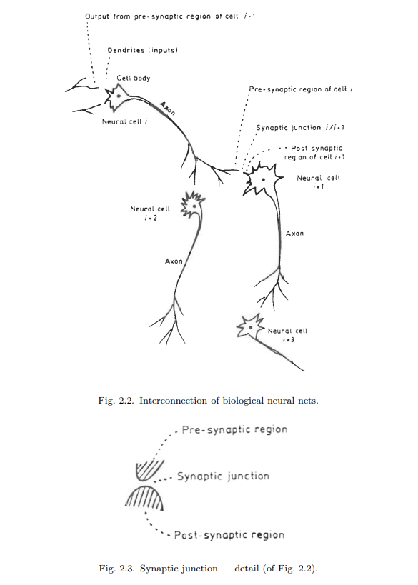
The biological neural network consists of nerve cells (neurons) as in Fig. 2.1, which are interconnected as in Fig. 2.2. The cell body of the neuron, which includes the neuron’s nucleus is where most of the neural “computation” takes place. Neural activity passes from one neuron to another in terms of electrical triggers which travel from one cell to the other down the neuron’s axon, by means of an electrochemical process of voltage-gated ion exchange along the axon and of diffusion of neurotransmitter molecules through the membrane over the synaptic gap (Fig. 2.3). The axon can be viewed as a connection wire. However, the mechanism of signal flow is not via electrical conduction but via charge exchange that is transported by diffusion of ions. This transportation process moves along the neuron’s cell, down the axon and then through synaptic junctions at the end of the axon via a very narrow synaptic space to the dendrites and/or soma of the next neuron at an average rate of $3 \mathrm{~m} / \mathrm{sec}$., as in Fig. 2.3 .

Figures 2.1 and 2.2 indicate that since a given neuron may have several (hundreds of) synapses, a neuron can connect (pass its message/signal) to many (hundreds of) other neurons. Similarly, since there are many dendrites per each neuron, a single

neuron can receive messages (neural signals) from many other neurons. In this manner, the biological neural network interconnects [Ganong, 1973].

It is important to note that not all interconnections, are equally weighted. Some have a higher priority (a higher weight) than others. Also some are excitory and some are inhibitory (serving to block transmission of a message). These differences are effected by differences in chemistry and by the existence of chemical transmitter and modulating substances inside and near the neurons, the axons and in the synaptic junction. This nature of interconnection between neurons and weighting of messages is also fundamental to artificial neural networks (ANNs).

计算机代写|神经网络代写neural networks代考|CS224W

神经网络代写

计算机代写|神经网络代写neural networks代考|Introduction and Role of Artificial Neural Networks

人工神经网络,顾名思义,是试图以粗略的方式模拟生物(人类或动物)中枢神经系统的神经细胞(神经元)网络的计算网络。这个模拟是一个细胞对细胞(神经元对神经元,元素对元素)的模拟。它借鉴了生物神经元和这种生物神经元网络的神经生理学知识。因此,它与传统的(数字或模拟)计算机器不同,传统的计算机器用来取代、增强或加速人脑的计算,而不考虑计算元素的组织和它们的网络。不过,我们要强调的是,神经网络提供的模拟是非常粗糙的。
那么,为什么我们要将人工神经网络(下文表示为神经网络或ANNs)视为不仅仅是模拟练习呢?我们必须问这个问题,特别是因为,在计算上(至少),传统的数字计算机可以做人工神经网络能做的一切。

答案在于两个重要的方面。神经网络通过模拟生物神经网络,实际上是一种相对于传统计算机而言的新型计算机体系结构和算法体系结构。它允许使用非常简单的计算操作(加法、乘法和基本逻辑元素)来解决复杂的、数学上不明确的问题、非线性问题或随机问题。传统的算法会使用复杂的方程组,只适用于一个给定的问题,并且完全适用于这个问题。人工神经网络将(a)在计算和算法上非常简单,(b)它将具有自组织特征,使其能够适用于广泛的问题。
例如,如果一只家蝇避开了一个障碍物,或者一只老鼠避开了一只猫,它当然不会求解轨迹上的微分方程,也不会使用复杂的模式识别算法。它的大脑非常简单,但它使用了一些基本的神经细胞,这些细胞从根本上服从于高级动物和人类的神经细胞结构。人工神经网络的解决方案也将以这种(很可能不是同样的)简单性为目标。阿尔伯特·爱因斯坦说,一个解决方案或模型必须尽可能简单,以适应手头的问题。尽管生物系统固有的速度很慢(它们的基本计算步骤大约需要一毫秒,而在今天的电子计算机中不到一纳秒),但为了像它们一样高效和通用,它们只能通过收敛到尽可能简单的算法架构来实现。高水平的数学和逻辑可以为解决方案提供一个广泛的通用框架,并可以简化为具体但复杂的算法,而神经网络的设计旨在最大限度地简单和最大限度地自组织。神经网络的基础算法结构非常简单,但它是一个高度适应广泛问题的算法结构。我们注意到,在目前的状态下,神经网络的自适应范围是有限的。然而,它们的设计是通过对生物网络的总体模拟来实现这种简单性和自组织的,而生物网络是(必须)由相同的原则指导的。

计算机代写|神经网络代写neural networks代考|Fundamentals of Biological Neural Networks

生物神经网络由神经细胞(神经元)组成,如图2.1所示,神经元之间相互连接,如图2.2所示。神经元的细胞体,包括神经元的细胞核,是大多数神经“计算”发生的地方。神经活动通过电触发器从一个神经元传递到另一个神经元,电触发器沿着神经元的轴突从一个细胞传递到另一个细胞,通过沿轴突电压门控离子交换的电化学过程和神经递质分子通过突触间隙上的膜扩散(图2.3)。轴突可以看作是一根连接线。然而,信号流动的机制不是通过电传导,而是通过离子扩散传递的电荷交换。这个运输过程沿着神经元的细胞,沿着轴突向下,然后通过轴突末端的突触连接,通过一个非常狭窄的突触空间,以平均$3 \ mathm {~m} / \ mathm {sec}$的速度到达下一个神经元的树突和/或体细胞。,如图2.3所示。

图2.1和2.2表明,由于一个给定的神经元可能有几个(数百个)突触,一个神经元可以连接(传递其信息/信号)到许多(数百个)其他神经元。同样的,因为每个神经元有很多树突,一个

一个神经元可以接收来自许多其他神经元的信息(神经信号)。以这种方式,生物神经网络相互连接[Ganong, 1973]。

重要的是要注意,并非所有的互连都具有相同的权重。有些优先级更高(权重更高)。还有一些是兴奋性的,一些是抑制性的(用于阻止信息的传递)。这些差异是由化学成分的差异以及神经元、轴突和突触连接处的化学递质和调节物质的存在所影响的。神经元之间的互连和信息加权的本质也是人工神经网络(ann)的基础。

计算机代写|神经网络代写neural networks代考 请认准statistics-lab™

统计代写请认准statistics-lab™. statistics-lab™为您的留学生涯保驾护航。

金融工程代写

金融工程是使用数学技术来解决金融问题。金融工程使用计算机科学、统计学、经济学和应用数学领域的工具和知识来解决当前的金融问题,以及设计新的和创新的金融产品。

非参数统计代写

非参数统计指的是一种统计方法,其中不假设数据来自于由少数参数决定的规定模型;这种模型的例子包括正态分布模型和线性回归模型。

广义线性模型代考

广义线性模型(GLM)归属统计学领域,是一种应用灵活的线性回归模型。该模型允许因变量的偏差分布有除了正态分布之外的其它分布。

术语 广义线性模型(GLM)通常是指给定连续和/或分类预测因素的连续响应变量的常规线性回归模型。它包括多元线性回归,以及方差分析和方差分析(仅含固定效应)。

有限元方法代写

有限元方法(FEM)是一种流行的方法,用于数值解决工程和数学建模中出现的微分方程。典型的问题领域包括结构分析、传热、流体流动、质量运输和电磁势等传统领域。

有限元是一种通用的数值方法,用于解决两个或三个空间变量的偏微分方程(即一些边界值问题)。为了解决一个问题,有限元将一个大系统细分为更小、更简单的部分,称为有限元。这是通过在空间维度上的特定空间离散化来实现的,它是通过构建对象的网格来实现的:用于求解的数值域,它有有限数量的点。边界值问题的有限元方法表述最终导致一个代数方程组。该方法在域上对未知函数进行逼近。[1] 然后将模拟这些有限元的简单方程组合成一个更大的方程系统,以模拟整个问题。然后,有限元通过变化微积分使相关的误差函数最小化来逼近一个解决方案。

tatistics-lab作为专业的留学生服务机构,多年来已为美国、英国、加拿大、澳洲等留学热门地的学生提供专业的学术服务,包括但不限于Essay代写,Assignment代写,Dissertation代写,Report代写,小组作业代写,Proposal代写,Paper代写,Presentation代写,计算机作业代写,论文修改和润色,网课代做,exam代考等等。写作范围涵盖高中,本科,研究生等海外留学全阶段,辐射金融,经济学,会计学,审计学,管理学等全球99%专业科目。写作团队既有专业英语母语作者,也有海外名校硕博留学生,每位写作老师都拥有过硬的语言能力,专业的学科背景和学术写作经验。我们承诺100%原创,100%专业,100%准时,100%满意。

随机分析代写


随机微积分是数学的一个分支,对随机过程进行操作。它允许为随机过程的积分定义一个关于随机过程的一致的积分理论。这个领域是由日本数学家伊藤清在第二次世界大战期间创建并开始的。

时间序列分析代写

随机过程,是依赖于参数的一组随机变量的全体,参数通常是时间。 随机变量是随机现象的数量表现,其时间序列是一组按照时间发生先后顺序进行排列的数据点序列。通常一组时间序列的时间间隔为一恒定值(如1秒,5分钟,12小时,7天,1年),因此时间序列可以作为离散时间数据进行分析处理。研究时间序列数据的意义在于现实中,往往需要研究某个事物其随时间发展变化的规律。这就需要通过研究该事物过去发展的历史记录,以得到其自身发展的规律。

回归分析代写

多元回归分析渐进(Multiple Regression Analysis Asymptotics)属于计量经济学领域,主要是一种数学上的统计分析方法,可以分析复杂情况下各影响因素的数学关系,在自然科学、社会和经济学等多个领域内应用广泛。

MATLAB代写

MATLAB 是一种用于技术计算的高性能语言。它将计算、可视化和编程集成在一个易于使用的环境中,其中问题和解决方案以熟悉的数学符号表示。典型用途包括:数学和计算算法开发建模、仿真和原型制作数据分析、探索和可视化科学和工程图形应用程序开发,包括图形用户界面构建MATLAB 是一个交互式系统,其基本数据元素是一个不需要维度的数组。这使您可以解决许多技术计算问题,尤其是那些具有矩阵和向量公式的问题,而只需用 C 或 Fortran 等标量非交互式语言编写程序所需的时间的一小部分。MATLAB 名称代表矩阵实验室。MATLAB 最初的编写目的是提供对由 LINPACK 和 EISPACK 项目开发的矩阵软件的轻松访问,这两个项目共同代表了矩阵计算软件的最新技术。MATLAB 经过多年的发展,得到了许多用户的投入。在大学环境中,它是数学、工程和科学入门和高级课程的标准教学工具。在工业领域,MATLAB 是高效研究、开发和分析的首选工具。MATLAB 具有一系列称为工具箱的特定于应用程序的解决方案。对于大多数 MATLAB 用户来说非常重要,工具箱允许您学习应用专业技术。工具箱是 MATLAB 函数(M 文件)的综合集合,可扩展 MATLAB 环境以解决特定类别的问题。可用工具箱的领域包括信号处理、控制系统、神经网络、模糊逻辑、小波、仿真等。

R语言代写问卷设计与分析代写
PYTHON代写回归分析与线性模型代写
MATLAB代写方差分析与试验设计代写
STATA代写机器学习/统计学习代写
SPSS代写计量经济学代写
EVIEWS代写时间序列分析代写
EXCEL代写深度学习代写
SQL代写各种数据建模与可视化代写

数学代写|复杂网络代写complex networks代考|CS7280

如果你也在 怎样代写复杂网络Complex Network 这个学科遇到相关的难题,请随时右上角联系我们的24/7代写客服。复杂网络Complex Network分析研究如何识别、描述、可视化和分析复杂网络。分析网络最突出的方法是使用Python库NetworkX,它为构造和绘制复杂的神经网络提供了一种突出的方法。

复杂网络Complex NetworkCNA研究和应用爆炸式增长的主要原因有两个因素:一是廉价而强大的计算机的可用性,使在数学、物理和社会科学方面受过高级培训的研究人员和科学家能够进行一流的研究;另一个因素是人类社会、行为、生物、金融和技术方面日益复杂。

statistics-lab™ 为您的留学生涯保驾护航 在代写复杂网络complex networks方面已经树立了自己的口碑, 保证靠谱, 高质且原创的统计Statistics代写服务。我们的专家在代写复杂网络complex networks方面经验极为丰富,各种代写复杂网络complex networks相关的作业也就用不着说。

数学代写|复杂网络代写complex networks代考|CS7280

数学代写|复杂网络代写complex networks代考|Benchmarking the Algorithm

In order to benchmark the performance of the Potts model approach to community detection, it is applied to computer-generated test networks. Networks with communities of equal and different size were constructed. Those with equal size had 128 nodes, grouped into 4 communities of size 32 . Those with differently sized communities had 320 nodes, grouped into 4 communities of size $32,64,96$ and 128 . In both types of networks, each node has an average degree of $\langle k\rangle=16$. The average number of links to members of the same community $\left\langle k_{i n}\right\rangle$ and to members of different communities $\left\langle k_{\text {out }}\right\rangle$ is then varied, but always ensuring $\left\langle k_{\text {in }}\right\rangle+\left\langle k_{\text {out }}\right\rangle=\langle k\rangle$. Hence, decreasing $k_{\text {in }}$ renders the problem of community detection more difficult.

Recovering a known community structure, any algorithm has to fulfill two criteria: it has to group nodes in the same community which belong together by design and it has to group nodes apart which belong to different communities by design. The first criterion is called “sensitivity” and measures the percentage of pairs of nodes which are correctly grouped together. The second criterion is called “specificity” and measures the percentage of pairs of nodes which are correctly grouped apart.

Because of the Poisson nature of the degree distribution, a connection model of $p_{i j}=p$ was used. Figure 4.5 shows the result of this experiment in comparison with the results obtained from the algorithm of Girvan and Newman [14]. Clearly, both algorithms show high sensitivity and high specificity. However, the Potts model outperforms the GN algorithm on both types of networks in both sensitivity and specificity. When relaxing the Potts model Hamiltonian from random initial conditions at zero temperature, performance decreases, but is still as good as that of the GN algorithm.

An important aspect is the dependence of the sensitivity (specificity) of the algorithm on the number of allowed spin states $q$. Figure 4.6 shows that as long as $q \geq 4$, i.e., the actual number of communities in the network, the value of $q$ is irrelevant. This result is also independent of the strength of the community structure under investigation, i.e., independent of $k_{i n}$. Furthermore, it is necessary to study the stability of results with respect to a change in $\gamma$. As Fig. 4.6 shows, the better the community structure is defined, i.e., the greater $k_{i n}$ is with respect to $\langle k\rangle$, the more stable are the results. The maxima of the curves for all values of $k_{i n}$, however, coincide at $\gamma=1$, i.e., at the point where the contribution of missing and existing links is equal. The same statements also apply to the specificity.

数学代写|复杂网络代写complex networks代考|Community Detection and Graph Partitioning

In order to assess the statistical significance of the community structures found with any algorithm, it is necessary to compare them with expectation values for random networks. This is of course always possible by rewiring the network randomly [15], keeping the degree distribution invariant and then running a community detection algorithm again, comparing the result to the original network. This method, however, can only give an answer to what a particular community detection algorithm may find in a random network and hence depends on the very method of community detection used. It seems a much better method would be to compare the results of a community detection algorithm with a theoretical result, obtained independently of any algorithm. It was shown in previous sections that the problem of community detection can be mapped onto finding the ground state of an infinite range spin glass. A number of techniques exist to calculate expectation values for the energy and the local field distribution in the ground state of spin glasses, given that the couplings between spins are random, but with a known distribution. In the remainder of this chapter and in the following ones, we will make extensive use of these techniques.

What does the community structure of a completely random network look like? The first observation one makes is that the configuration space or the number of possible assignments into $q$ communities is largest when these groups are equal in size, i.e., contain the same number of nodes $N / q$. One can also show that the variance of the number of links within communities is largest when they are of equal size. These two facts taken together mean that in random networks, the assignment of nodes into communities with maximal modularity will with very high probability lead to equal-sized communities. Hence, we only need to calculate expectation values for the modularity of a partition of the network into equal-sized groups. In the language of spin glasses, this means we are looking for the energy of a ground state with zero magnetization. We can also say that we are looking for a partition into $q$ equal-sized groups with a maximum number of links within groups, or, equivalently, with a minimum number of links between groups. The latter is a standard problem in combinatorial optimization and is known as the graph partitioning problem. In short, the communities which form the partition of maximum modularity in a random network will correspond to a minimum cut equipartition.

数学代写|复杂网络代写complex networks代考|CS7280

数学代写|复杂网络代写complex networks代考|Benchmarking the Algorithm

为了测试Potts模型在社区检测中的性能,将其应用于计算机生成的测试网络。构建了大小不等的社区网络。大小相同的有128个节点,分成4个32个节点的社区。不同大小的群落有320个节点,分为4个群落,大小分别为$32,64,96$和128。在这两种类型的网络中,每个节点的平均度为$\langle k\rangle=16$。到同一社区成员$\left\langle k_{i n}\right\rangle$和不同社区成员$\left\langle k_{\text {out }}\right\rangle$的平均链接数是不同的,但始终确保$\left\langle k_{\text {in }}\right\rangle+\left\langle k_{\text {out }}\right\rangle=\langle k\rangle$。因此,减少$k_{\text {in }}$使得社区检测问题更加困难。

恢复一个已知的社区结构,任何算法都必须满足两个标准:它必须将同一社区中的节点按照设计分组在一起,并且必须将属于不同社区的节点按照设计分组分开。第一个标准被称为“灵敏度”,衡量正确组合在一起的节点对的百分比。第二个标准被称为“特异性”,衡量正确分组的节点对的百分比。

由于度分布的泊松性质,使用$p_{i j}=p$的连接模型。图4.5为本实验结果与Girvan和Newman[14]算法结果的对比。显然,这两种算法都具有高灵敏度和高特异性。然而,Potts模型在两种类型的网络上的敏感性和特异性都优于GN算法。当在零温度下从随机初始条件放宽Potts模型哈密顿量时,性能下降,但仍然与GN算法一样好。

一个重要的方面是该算法的灵敏度(特异性)依赖于允许的自旋态的数量$q$。从图4.6可以看出,只要$q \geq 4$即网络中社区的实际数量,$q$的值就无关紧要。该结果也独立于所调查的社区结构的强度,即独立于$k_{i n}$。此外,有必要研究结果相对于$\gamma$的变化的稳定性。如图4.6所示,群落结构定义得越好,即$k_{i n}$相对于$\langle k\rangle$越大,则结果越稳定。然而,所有$k_{i n}$值的曲线的最大值在$\gamma=1$重合,即在缺失链接和现有链接的贡献相等的点上。同样的陈述也适用于特异性。

数学代写|复杂网络代写complex networks代考|Community Detection and Graph Partitioning

为了评估用任何算法找到的群体结构的统计显著性,有必要将它们与随机网络的期望值进行比较。当然,这总是可以通过随机重新连接网络来实现[15],保持度分布不变,然后再次运行社区检测算法,将结果与原始网络进行比较。然而,这种方法只能给出特定社区检测算法在随机网络中可能发现的答案,因此取决于所使用的社区检测方法。似乎更好的方法是将社区检测算法的结果与独立于任何算法获得的理论结果进行比较。在前面的章节中已经表明,共同体检测的问题可以映射到寻找无限范围自旋玻璃的基态。考虑到自旋玻璃之间的耦合是随机的,但有一个已知的分布,存在许多技术来计算自旋玻璃基态的能量和局部场分布的期望值。在本章的剩余部分和以下几章中,我们将广泛使用这些技术。

一个完全随机网络的社区结构是什么样的?第一个观察结果是,当这些组的大小相等时,配置空间或可能分配到$q$社区的数量最大,即包含相同数量的节点$N / q$。我们还可以证明,当社区内的链接大小相等时,它们的数量差异最大。这两个事实结合在一起意味着,在随机网络中,将节点分配到具有最大模块化的社区将有很大的概率导致等大小的社区。因此,我们只需要计算网络划分为大小相等的组的模块化的期望值。在自旋玻璃的语言中,这意味着我们正在寻找具有零磁化的基态的能量。我们也可以说,我们正在寻找一个划分为$q$大小相等的组,组内具有最大数量的链接,或者,等价地,组之间具有最小数量的链接。后者是组合优化中的一个标准问题,被称为图划分问题。简而言之,在一个随机网络中,组成最大模块划分的社团对应于一个最小切割均分。

统计代写|复杂网络代写complex networks代考 请认准statistics-lab™

统计代写请认准statistics-lab™. statistics-lab™为您的留学生涯保驾护航。统计代写|python代写代考

随机过程代考

在概率论概念中,随机过程随机变量的集合。 若一随机系统的样本点是随机函数,则称此函数为样本函数,这一随机系统全部样本函数的集合是一个随机过程。 实际应用中,样本函数的一般定义在时间域或者空间域。 随机过程的实例如股票和汇率的波动、语音信号、视频信号、体温的变化,随机运动如布朗运动、随机徘徊等等。

贝叶斯方法代考

贝叶斯统计概念及数据分析表示使用概率陈述回答有关未知参数的研究问题以及统计范式。后验分布包括关于参数的先验分布,和基于观测数据提供关于参数的信息似然模型。根据选择的先验分布和似然模型,后验分布可以解析或近似,例如,马尔科夫链蒙特卡罗 (MCMC) 方法之一。贝叶斯统计概念及数据分析使用后验分布来形成模型参数的各种摘要,包括点估计,如后验平均值、中位数、百分位数和称为可信区间的区间估计。此外,所有关于模型参数的统计检验都可以表示为基于估计后验分布的概率报表。

广义线性模型代考

广义线性模型(GLM)归属统计学领域,是一种应用灵活的线性回归模型。该模型允许因变量的偏差分布有除了正态分布之外的其它分布。

statistics-lab作为专业的留学生服务机构,多年来已为美国、英国、加拿大、澳洲等留学热门地的学生提供专业的学术服务,包括但不限于Essay代写,Assignment代写,Dissertation代写,Report代写,小组作业代写,Proposal代写,Paper代写,Presentation代写,计算机作业代写,论文修改和润色,网课代做,exam代考等等。写作范围涵盖高中,本科,研究生等海外留学全阶段,辐射金融,经济学,会计学,审计学,管理学等全球99%专业科目。写作团队既有专业英语母语作者,也有海外名校硕博留学生,每位写作老师都拥有过硬的语言能力,专业的学科背景和学术写作经验。我们承诺100%原创,100%专业,100%准时,100%满意。

机器学习代写

随着AI的大潮到来,Machine Learning逐渐成为一个新的学习热点。同时与传统CS相比,Machine Learning在其他领域也有着广泛的应用,因此这门学科成为不仅折磨CS专业同学的“小恶魔”,也是折磨生物、化学、统计等其他学科留学生的“大魔王”。学习Machine learning的一大绊脚石在于使用语言众多,跨学科范围广,所以学习起来尤其困难。但是不管你在学习Machine Learning时遇到任何难题,StudyGate专业导师团队都能为你轻松解决。

多元统计分析代考


基础数据: $N$ 个样本, $P$ 个变量数的单样本,组成的横列的数据表
变量定性: 分类和顺序;变量定量:数值
数学公式的角度分为: 因变量与自变量

时间序列分析代写

随机过程,是依赖于参数的一组随机变量的全体,参数通常是时间。 随机变量是随机现象的数量表现,其时间序列是一组按照时间发生先后顺序进行排列的数据点序列。通常一组时间序列的时间间隔为一恒定值(如1秒,5分钟,12小时,7天,1年),因此时间序列可以作为离散时间数据进行分析处理。研究时间序列数据的意义在于现实中,往往需要研究某个事物其随时间发展变化的规律。这就需要通过研究该事物过去发展的历史记录,以得到其自身发展的规律。

回归分析代写

多元回归分析渐进(Multiple Regression Analysis Asymptotics)属于计量经济学领域,主要是一种数学上的统计分析方法,可以分析复杂情况下各影响因素的数学关系,在自然科学、社会和经济学等多个领域内应用广泛。

MATLAB代写

MATLAB 是一种用于技术计算的高性能语言。它将计算、可视化和编程集成在一个易于使用的环境中,其中问题和解决方案以熟悉的数学符号表示。典型用途包括:数学和计算算法开发建模、仿真和原型制作数据分析、探索和可视化科学和工程图形应用程序开发,包括图形用户界面构建MATLAB 是一个交互式系统,其基本数据元素是一个不需要维度的数组。这使您可以解决许多技术计算问题,尤其是那些具有矩阵和向量公式的问题,而只需用 C 或 Fortran 等标量非交互式语言编写程序所需的时间的一小部分。MATLAB 名称代表矩阵实验室。MATLAB 最初的编写目的是提供对由 LINPACK 和 EISPACK 项目开发的矩阵软件的轻松访问,这两个项目共同代表了矩阵计算软件的最新技术。MATLAB 经过多年的发展,得到了许多用户的投入。在大学环境中,它是数学、工程和科学入门和高级课程的标准教学工具。在工业领域,MATLAB 是高效研究、开发和分析的首选工具。MATLAB 具有一系列称为工具箱的特定于应用程序的解决方案。对于大多数 MATLAB 用户来说非常重要,工具箱允许您学习应用专业技术。工具箱是 MATLAB 函数(M 文件)的综合集合,可扩展 MATLAB 环境以解决特定类别的问题。可用工具箱的领域包括信号处理、控制系统、神经网络、模糊逻辑、小波、仿真等。

R语言代写问卷设计与分析代写
PYTHON代写回归分析与线性模型代写
MATLAB代写方差分析与试验设计代写
STATA代写机器学习/统计学习代写
SPSS代写计量经济学代写
EVIEWS代写时间序列分析代写
EXCEL代写深度学习代写
SQL代写各种数据建模与可视化代写

统计代写|复杂网络代写complex networks代考|CS60078

如果你也在 怎样代写复杂网络Complex Network 这个学科遇到相关的难题,请随时右上角联系我们的24/7代写客服。复杂网络Complex Network分析研究如何识别、描述、可视化和分析复杂网络。分析网络最突出的方法是使用Python库NetworkX,它为构造和绘制复杂的神经网络提供了一种突出的方法。

复杂网络Complex NetworkCNA研究和应用爆炸式增长的主要原因有两个因素:一是廉价而强大的计算机的可用性,使在数学、物理和社会科学方面受过高级培训的研究人员和科学家能够进行一流的研究;另一个因素是人类社会、行为、生物、金融和技术方面日益复杂。

statistics-lab™ 为您的留学生涯保驾护航 在代写复杂网络complex networks方面已经树立了自己的口碑, 保证靠谱, 高质且原创的统计Statistics代写服务。我们的专家在代写复杂网络complex networks方面经验极为丰富,各种代写复杂网络complex networks相关的作业也就用不着说。

统计代写|复杂网络代写complex networks代考|CS60078

统计代写|复杂网络代写complex networks代考|Non-hierarchical

The non-hierarchical methods approach the problem from a different perspective. In principle, they intend to calculate a full distance matrix for the nodes of the network. This can then be treated by conventional techniques.

One of the earliest approaches to community detection is due to Eriksen et al. $[41,42]$. They study a diffusion process on a network and analyze the decay of the modes of the following diffusive system with discrete time:

$$
\rho_i(t+1)-\rho_i(t)=\sum_j\left(T_{i j}-\delta_{i j}\right) \rho_j(t) .
$$
Here $T_{i j}$ represents the adjacency matrix of the network such that $T_{i j}=1 / k_j$ for $A_{i j}=1$ and zero otherwise. Hence $T_{i j}$ represents the probability of a random walker to go from $j$ to $i$. The decay of a random initial configuration $\rho(t=0)$ toward the steady state is characterized by the eigenmodes of the transition matrix $T_{i j}$. The eigenvectors corresponding to the largest eigenvalues can then be used to define a distance between nodes which helps in identifying communities. To do this, the eigenvectors belonging to the largest non-trivial positive eigenvalues are plotted against each other. This diffusion approach is very similar in spirit to other algorithms based on the idea of using flow simulations for community detection as suggested by van Dongen [43] under the name of “Markov clustering” (MCL).

The method presented by Zhou [44-46] first converts the sparse adjacency matrix of the graph into a full distance matrix by calculating the average time a Brownian particle needs to move from node $i$ to $j$. Then this distance matrix is clustered using ordinary hierarchical clustering algorithms. This approach is based on the observation that a random walker has shorter traveling time between two nodes if many (short) alternative paths exist.

Another spectral approach has been taken by Muños and Donetti [47]. They work with the Laplacian matrix of the network. The Laplacian is defined as
$$
L_{i j}=k_i \delta_{i j}-A_{i j} .
$$

统计代写|复杂网络代写complex networks代考|Optimization Based

A different approach which is reminiscent of the parametric clustering procedures known in computer science is the idea of searching for partitions with maximum modularity $Q$ using combinatorial optimization techniques [48]. This approach has been adopted by Guimera et al. in Refs. [2, 49] or Massen et al. [50] using simulated annealing [51] or Duch and Arenas using extremal optimization [52].

Though this approach will be the preferred one for the remainder of this book, a number of issues remain. For the hierarchical algorithms, a community was to be understood as whatever the algorithm outputs. Now, it is not the algorithm that defines what a community is, but the quality function, i.e., the modularity $Q$ in this case. Also, the modularity $Q$ as defined by Newman $[23]$ is parameter free and an understanding for hierarchical and overlapping structures needs to be developed.

Block structure in networks is a very common and well-studied phenomenon. The concepts of structural and regular equivalence as well as the types of blocks defined for generalized block modeling are well defined but appear too rigid to be of practical use for large and noisy data sets. Diagonal block models or modular structures have received particular attention in the literature and have developed into an almost independent concept of cohesive subgroups or communities. The comparison of many different community definitions from various fields has shown that the concept of module or community in a network is only vaguely defined. The diversity of algorithms published is only a consequence of this vague definition. None of the algorithms could be called “ideal” in the sense that it combines the features of computational efficiency, accuracy, flexibility and adaptability with regard to the network and easy interpretation of the results. More importantly, none of the above-cited publications allows an estimation to which degree the community structure found is a reality of the network or a product of the clustering process itself. The following chapters are addressing these issues and present a framework in which community detection is viewed again as a special case of a general procedure for detecting block structure in networks.

统计代写|复杂网络代写complex networks代考|CS60078

复杂网络代写

统计代写|复杂网络代写complex networks代考|Non-hierarchical

非分层方法从不同的角度处理问题。原则上,他们打算计算网络节点的全距离矩阵。然后可以用常规技术来处理。

最早的社区检测方法之一来自Eriksen等人$[41,42]$。他们研究了网络上的扩散过程,并分析了以下扩散系统的模态随离散时间的衰减:

$$
\rho_i(t+1)-\rho_i(t)=\sum_j\left(T_{i j}-\delta_{i j}\right) \rho_j(t) .
$$
这里$T_{i j}$表示网络的邻接矩阵,使得$A_{i j}=1$为$T_{i j}=1 / k_j$,否则为零。因此$T_{i j}$表示随机步行者从$j$到$i$的概率。随机初始构型$\rho(t=0)$向稳态的衰减由跃迁矩阵$T_{i j}$的特征模态表征。与最大特征值相对应的特征向量可以用来定义节点之间的距离,这有助于识别社区。为了做到这一点,属于最大非平凡正特征值的特征向量被相互绘制。这种扩散方法在精神上与van Dongen[43]以“马尔可夫聚类”(Markov clustering, MCL)的名义提出的基于使用流模拟进行社区检测的思想的其他算法非常相似。

Zhou[44-46]提出的方法首先通过计算布朗粒子从节点$i$移动到$j$所需的平均时间,将图的稀疏邻接矩阵转换为全距离矩阵。然后使用普通的层次聚类算法对该距离矩阵进行聚类。这种方法是基于这样的观察:如果存在许多(短)可选路径,则随机行走器在两个节点之间的行走时间会更短。

Muños和Donetti[47]采用了另一种光谱方法。他们使用网络的拉普拉斯矩阵。拉普拉斯式定义为
$$
L_{i j}=k_i \delta_{i j}-A_{i j} .
$$

统计代写|复杂网络代写complex networks代考|Optimization Based

另一种与计算机科学中已知的参数聚类过程类似的方法是使用组合优化技术搜索具有最大模块化$Q$的分区[48]。Guimera等人在参考文献中采用了这种方法。[2,49]或Massen等[50]使用模拟退火[51]或Duch和Arenas使用极值优化[52]。

尽管这种方法将是本书其余部分的首选方法,但仍然存在一些问题。对于分层算法,社区被理解为算法的输出。现在,定义社区的不是算法,而是质量函数,即本例中的模块化Q。此外,Newman $[23]定义的模块化$Q$是无参数的,需要发展对分层和重叠结构的理解。

网络中的块结构是一种非常普遍且被充分研究的现象。结构等价和规则等价的概念以及为广义块建模定义的块的类型都有很好的定义,但对于大型和有噪声的数据集来说,似乎过于严格而无法实际使用。对角块模型或模块化结构在文献中受到了特别的关注,并已发展成为一个几乎独立的凝聚力子群体或社区的概念。通过比较不同领域对社区的定义,可以发现网络中模块或社区的定义是模糊的。发表的算法的多样性只是这种模糊定义的结果。没有一种算法可以被称为“理想”,因为它结合了计算效率、准确性、灵活性和网络适应性以及易于解释结果的特点。更重要的是,上述引用的出版物都不允许估计发现的社区结构在多大程度上是网络的现实或聚类过程本身的产物。下面的章节将讨论这些问题,并提出一个框架,在这个框架中,社区检测再次被视为检测网络中块结构的一般程序的特殊情况。

统计代写|复杂网络代写complex networks代考 请认准statistics-lab™

统计代写请认准statistics-lab™. statistics-lab™为您的留学生涯保驾护航。统计代写|python代写代考

随机过程代考

在概率论概念中,随机过程随机变量的集合。 若一随机系统的样本点是随机函数,则称此函数为样本函数,这一随机系统全部样本函数的集合是一个随机过程。 实际应用中,样本函数的一般定义在时间域或者空间域。 随机过程的实例如股票和汇率的波动、语音信号、视频信号、体温的变化,随机运动如布朗运动、随机徘徊等等。

贝叶斯方法代考

贝叶斯统计概念及数据分析表示使用概率陈述回答有关未知参数的研究问题以及统计范式。后验分布包括关于参数的先验分布,和基于观测数据提供关于参数的信息似然模型。根据选择的先验分布和似然模型,后验分布可以解析或近似,例如,马尔科夫链蒙特卡罗 (MCMC) 方法之一。贝叶斯统计概念及数据分析使用后验分布来形成模型参数的各种摘要,包括点估计,如后验平均值、中位数、百分位数和称为可信区间的区间估计。此外,所有关于模型参数的统计检验都可以表示为基于估计后验分布的概率报表。

广义线性模型代考

广义线性模型(GLM)归属统计学领域,是一种应用灵活的线性回归模型。该模型允许因变量的偏差分布有除了正态分布之外的其它分布。

statistics-lab作为专业的留学生服务机构,多年来已为美国、英国、加拿大、澳洲等留学热门地的学生提供专业的学术服务,包括但不限于Essay代写,Assignment代写,Dissertation代写,Report代写,小组作业代写,Proposal代写,Paper代写,Presentation代写,计算机作业代写,论文修改和润色,网课代做,exam代考等等。写作范围涵盖高中,本科,研究生等海外留学全阶段,辐射金融,经济学,会计学,审计学,管理学等全球99%专业科目。写作团队既有专业英语母语作者,也有海外名校硕博留学生,每位写作老师都拥有过硬的语言能力,专业的学科背景和学术写作经验。我们承诺100%原创,100%专业,100%准时,100%满意。

机器学习代写

随着AI的大潮到来,Machine Learning逐渐成为一个新的学习热点。同时与传统CS相比,Machine Learning在其他领域也有着广泛的应用,因此这门学科成为不仅折磨CS专业同学的“小恶魔”,也是折磨生物、化学、统计等其他学科留学生的“大魔王”。学习Machine learning的一大绊脚石在于使用语言众多,跨学科范围广,所以学习起来尤其困难。但是不管你在学习Machine Learning时遇到任何难题,StudyGate专业导师团队都能为你轻松解决。

多元统计分析代考


基础数据: $N$ 个样本, $P$ 个变量数的单样本,组成的横列的数据表
变量定性: 分类和顺序;变量定量:数值
数学公式的角度分为: 因变量与自变量

时间序列分析代写

随机过程,是依赖于参数的一组随机变量的全体,参数通常是时间。 随机变量是随机现象的数量表现,其时间序列是一组按照时间发生先后顺序进行排列的数据点序列。通常一组时间序列的时间间隔为一恒定值(如1秒,5分钟,12小时,7天,1年),因此时间序列可以作为离散时间数据进行分析处理。研究时间序列数据的意义在于现实中,往往需要研究某个事物其随时间发展变化的规律。这就需要通过研究该事物过去发展的历史记录,以得到其自身发展的规律。

回归分析代写

多元回归分析渐进(Multiple Regression Analysis Asymptotics)属于计量经济学领域,主要是一种数学上的统计分析方法,可以分析复杂情况下各影响因素的数学关系,在自然科学、社会和经济学等多个领域内应用广泛。

MATLAB代写

MATLAB 是一种用于技术计算的高性能语言。它将计算、可视化和编程集成在一个易于使用的环境中,其中问题和解决方案以熟悉的数学符号表示。典型用途包括:数学和计算算法开发建模、仿真和原型制作数据分析、探索和可视化科学和工程图形应用程序开发,包括图形用户界面构建MATLAB 是一个交互式系统,其基本数据元素是一个不需要维度的数组。这使您可以解决许多技术计算问题,尤其是那些具有矩阵和向量公式的问题,而只需用 C 或 Fortran 等标量非交互式语言编写程序所需的时间的一小部分。MATLAB 名称代表矩阵实验室。MATLAB 最初的编写目的是提供对由 LINPACK 和 EISPACK 项目开发的矩阵软件的轻松访问,这两个项目共同代表了矩阵计算软件的最新技术。MATLAB 经过多年的发展,得到了许多用户的投入。在大学环境中,它是数学、工程和科学入门和高级课程的标准教学工具。在工业领域,MATLAB 是高效研究、开发和分析的首选工具。MATLAB 具有一系列称为工具箱的特定于应用程序的解决方案。对于大多数 MATLAB 用户来说非常重要,工具箱允许您学习应用专业技术。工具箱是 MATLAB 函数(M 文件)的综合集合,可扩展 MATLAB 环境以解决特定类别的问题。可用工具箱的领域包括信号处理、控制系统、神经网络、模糊逻辑、小波、仿真等。

R语言代写问卷设计与分析代写
PYTHON代写回归分析与线性模型代写
MATLAB代写方差分析与试验设计代写
STATA代写机器学习/统计学习代写
SPSS代写计量经济学代写
EVIEWS代写时间序列分析代写
EXCEL代写深度学习代写
SQL代写各种数据建模与可视化代写

统计代写|网络分析代写Network Analysis代考|Graphical Analysis

如果你也在 怎样代写网络分析Network Analysis这个学科遇到相关的难题,请随时右上角联系我们的24/7代写客服。

网络分析研究实体之间的关系,如个人、组织或文件。在多个层面上操作,它描述并推断单个实体、实体的子集和整个网络的关系属性。

statistics-lab™ 为您的留学生涯保驾护航 在代写网络分析Network Analysis方面已经树立了自己的口碑, 保证靠谱, 高质且原创的统计Statistics代写服务。我们的专家在代写网络分析Network Analysis代写方面经验极为丰富,各种代写网络分析Network Analysis相关的作业也就用不着说。

我们提供的网络分析Network Analysis及其相关学科的代写,服务范围广, 其中包括但不限于:

  • Statistical Inference 统计推断
  • Statistical Computing 统计计算
  • Advanced Probability Theory 高等概率论
  • Advanced Mathematical Statistics 高等数理统计学
  • (Generalized) Linear Models 广义线性模型
  • Statistical Machine Learning 统计机器学习
  • Longitudinal Data Analysis 纵向数据分析
  • Foundations of Data Science 数据科学基础

统计代写|网络分析代写Network Analysis代考|Bipartite Graphs of Host Communications

Host communications observed in network traffic of Internet links could be naturally modeled with a bipartite graph $\mathcal{G}=(\mathcal{A}, \mathcal{B}, \mathcal{E})$, where $\mathcal{A}$ and $\mathcal{B}$ are two disjoint vertex sets, and $\mathcal{E} \subseteq \mathcal{A} \times \mathcal{B}$ is the edge set [35]. Specifically, all the source IP addresses observed in network traffic from one single direction of an Internet link form the vertex set $\mathcal{A}$, while the vertex set $\mathcal{B}$ consists of all the destination addresses observed in the same traffic. Each of the edges, $e_k$ in $\mathcal{G}$ connects one vertex $a_i \in \mathcal{A}$ and another vertex $b_j \in \mathcal{B}$.

Figure 2.2 illustrates an example of a simple bipartite graph that shows data communications between six source IP addresses $\left(s_1-s_6\right)$ and four destination IP addresses $\left(d_1-d_4\right)$. Note that an Internet link carries network traffic from two directions, thus we separate network traffic based on traffic directions and use bipartite graphs to model network traffic from two directions separately.

To study the social-behavior similarity of end hosts in network traffic, we leverage one-mode projection graphs of bipartite graphs that are used to extract hidden information or relationships between nodes within the same vertex sets [35]. Figure 2.3[a] illustrates the one-mode projection of the bipartite graph on the vertex set of the six left-side nodes, i.e., the source hosts $\left(s_1-s_6\right)$ in Fig. 2.2, while Fig. 2.3 [b] is the onemode projection on the four destination hosts $d_1-d_4$ in Fig. 2.2. An edge connects two nodes in the one-mode projection if and only if both nodes have connections to at least one same node in the bipartite graph. Thus studying one-mode projection graphs could potentially reveal the similarity or dissimilarity of communication patterns and traffic behaviors for networked systems and Internet applications.

统计代写|网络分析代写Network Analysis代考|Adaptive Thresholding Algorithm

We start by focusing on each dimension of the four-feature space, srCIP, dstIP, srcPrt, or dstPrt, and extract significant clusters of interest along this dimension. The extracted srCIP and dstIP clusters yield a set of interesting host behaviors (communication patterns), while the srcPrt and dstPrt clusters yield a set of interesting service/port behaviors, reflecting the aggregate behaviors of individual hosts on the corresponding ports. In the following, we introduce our definition of significance/interestingness using the (conditional) relative uncertainty measure (cf. Appendix A).

Given one feature dimension $X$ and a time interval $T$, let $m$ be the total number of flows observed during the time interval, and $A=\left{a_1, \ldots, a_n\right}, n \geq 2$, be the set of distinct values (e.g., srcIP’s) in $X$ that the observed flows take. Then the (induced) probability distribution $\mathcal{P}_A$ on $X$ is given by $p_i:=\mathcal{P}_A\left(a_i\right)=m_i / m$, where $m_i$ is the number of flows that take the value $a_i$ (e.g., having the $\left.\operatorname{srcIP} a_i\right)$. Then the (conditional) relative uncertainty, $R U\left(\mathcal{P}_A\right):=R U(X \mid A)$, measures the degree of uniformity in the observed features $A$. If $R U\left(\mathcal{P}_A\right)$ is close to 1 , say, $>\beta=0.9$, then the observed values are close to being uniformly distributed, and thus nearly indistinguishable. Otherwise, there are likely feature values in $A$ that “stand out” from the rest. We say a subset $S$ of $A$ contains the most significant (thus “interesting”) values of $A$ if $S$ is the smallest subset of $A$ such that (i) the probability of any value in $S$ is larger than those of the remaining values; and (ii) the (conditional) probability distribution on the set of the remaining values, $R:=A-S$, is close to being uniformly distributed, i.e., $R U\left(\mathcal{P}_R\right):=R U(X \mid R)>\beta$. Intuitively, $S$ contains the most significant feature values in $A$, while the remaining values are nearly indistinguishable from each other.

To see what $S$ contains, order the feature values of $A$ based on their probabilities: let $\hat{a}1, \hat{a}_2, \ldots, \hat{a}_n$ be such as $\mathcal{P}_A\left(\hat{a}_1\right) \geq \mathcal{P}_A\left(\hat{a}_2\right) \geq \ldots \mathcal{P}_A\left(\hat{a}_n\right)$. Then $S=$ $\left{\hat{a}_1, \hat{a}_2, \ldots, \hat{a}{k-1}\right}$, and $R=A-S=\left{\hat{a}k, \hat{a}{k+1}, \ldots, \hat{a}n\right}$, where $k$ is the smallest integer such that $R U\left(\mathcal{P}_R\right)>\beta$. Let $\alpha^=\hat{a}{k-1}$. Then $\alpha^$ is the largest “cut-off” threshold such that the (conditional) probability distribution on the set of remaining values $R$ is close to being uniformly distributed. To extract $S$ from $A$ (thereby, the clusters of flows associated with the significant feature values), we take advantage of the fact that in practice the probability distribution of the feature values $\mathcal{P}_A$ in general obeys a power-law: only a relatively few values (with respect to $n$ ) have significant larger probabilities, i.e., $|S|$ is relatively small, while the remaining feature values are close to being uniformly distributed. Hence, we can efficiently search for the optimal cut-off threshold $\alpha^*$.

网络分析代考

统计代写|网络分析代写Network Analysis代考|Bipartite Graphs of Host Communications

在 Internet 链接的网络流量中观察到的主机通信可以自然地用二分图建模 $\mathcal{G}=(\mathcal{A}, \mathcal{B}, \mathcal{E})$ ,在哪里 $\mathcal{A}$ 和 $\mathcal{B}$ 是 两个不相交的顶点集,并且 $\mathcal{E} \subseteq \mathcal{A} \times \mathcal{B}$ 是边集[35]。具体来说,从互联网链路的一个方向的网络流量中观察 到的所有源 $\mathrm{I}$ 地址构成顶点集 $\mathcal{A}$, 而顶点集 $\mathcal{B}$ 由在同一流量中观察到的所有目标地址组成。每一个边缘, $e_k$ 在 $\mathcal{G}$ 连接一个顶点 $a_i \in \mathcal{A}$ 和另一个顶点 $b_j \in \mathcal{B}$.
图 2.2 展示了一个简单的二分图示例,其中显示了六个源 IP 地址之间的数据通信 $\left(s_1-s_6\right)$ 和四个目标 IP 地 址 $\left(d_1-d_4\right)$. 请注意,互联网链路承载来自两个方向的网络流量,因此我们根据流量方向分离网络流量,并 使用二分图分别对来自两个方向的网络流量进行建模。
为了研究网络流量中终端主机的社会行为相似性,我们利用二分图的单模式投影图,这些图用于提取隐藏信 息或同一顶点集中节点之间的关系 [35]。图2.3[a]说明了二部图在六个左侧节点即源主机的顶点集上的单模投 影 $\left(s_1-s_6\right)$ 在图 2.2 中,而图 2.3 [b] 是在四个目标主机上的单模投影 $d_1-d_4$ 在图 2.2 中。当且仅当两个 节点都连接到二分图中的至少一个相同节点时,一条边连接单模投影中的两个节点。因此,研究单模投影图 可能会揭示网络系统和 Internet 应用程序的通信模式和流量行为的相似性或不同性。

统计代写|网络分析代写Network Analysis代考|Adaptive Thresholding Algorithm

我们首先关注四特征空间的每个维度,srCIP、dstIP、srcPrt 或 dstPrt,并沿着该维度提取重要的兴趣聚类。 提取的 srCIP 和 dstIP 集群产生了一组有趣的主机行为(通信模式),而 srcPrt 和 dstPrt 集群产生了一组有 趣的服务/端口行为,反映了各个主机在相应端口上的聚合行为。在下文中,我们使用 (条件) 相对不确定性 度量(参见附录 A) 介绍我们对重要性/兴趣的定义。
给定一个特征维度 $X$ 和一个时间间隔 $T$ ,让 $m$ 是在时间间隔内观察到的流量总数,并且 分布 $\mathcal{P}_A$ 在 $X$ 是 (谁) 给的 $p_i:=\mathcal{P}_A\left(a_i\right)=m_i / m$ ,在哪里 $m_i$ 是取值的流数 $a_i$ (例如,有 $\operatorname{srcIP} a_i$ ). 那 么 (有条件的) 相对不确定性, $R U\left(\mathcal{P}_A\right):=R U(X \mid A)$ ,测量观察到的特征的均匀程度 $A$. 如果 $R U\left(\mathcal{P}_A\right)$ 接近于 1,比方说, $>\beta=0.9$ ,则观测值接近均匀分布,因此几乎无法区分。否则,可能有特 征值 $A$ 从其他人中“脱颕而出”。我们说一个子集 $S$ 的 $A$ 包含最重要(因此“有趣”)的值 $A$ 如果 $S$ 是的最小子集 $A$ 这样 (i) 中任何值的概率 $S$ 大于其余值;(ii) 剩余值集合的 (条件) 概率分布, $R:=A-S$, 接近于均匀分 布,即 $R U\left(\mathcal{P}_R\right):=R U(X \mid R)>\beta$. 直觉上, $S$ 包含最重要的特征值 $A$ ,而其余值几乎无法区分。
看什么 $S$ 包含,排序的特征值 $A$ 基于他们的概率:让 $\hat{a} 1, \hat{a}_2, \ldots, \hat{a}_n$ 是例如 $\mathrm{R}=\mathrm{AS}=\backslash$ left ${$ hat ${a} k$, \hat ${a}{k+1}$, \dots, \hat ${a} n \backslash r i g h t}$ , 在哪里 $k$ 是满足以下条件的最小整数 $R U\left(\mathcal{P}_R\right)>\beta$. 让 $\alpha^{=} \hat{a} k-1$. 然同 1 阿尔法^ 是最大的“截止”阈值,使得剩余值集上的(条件)概率分布 $R$ 接近均匀分布。提 取 $S$ 从 $A$ (因此,流的集群与重要的特征值相关联),我们利用了这样一个事实,即在实践中特征值的概率分 布 $\mathcal{P}_A$ 一般来说服从幂律:只有相对较少的值(相对于 $n$ ) 具有显着更大的概率,即 $|S|$ 相对较小,而其余特征 值接近均匀分布。因此,我们可以有效地搜索最佳截止阈值 $\alpha^*$.

统计代写|网络分析代写Network Analysis代考 请认准statistics-lab™

统计代写请认准statistics-lab™. statistics-lab™为您的留学生涯保驾护航。

金融工程代写

金融工程是使用数学技术来解决金融问题。金融工程使用计算机科学、统计学、经济学和应用数学领域的工具和知识来解决当前的金融问题,以及设计新的和创新的金融产品。

非参数统计代写

非参数统计指的是一种统计方法,其中不假设数据来自于由少数参数决定的规定模型;这种模型的例子包括正态分布模型和线性回归模型。

广义线性模型代考

广义线性模型(GLM)归属统计学领域,是一种应用灵活的线性回归模型。该模型允许因变量的偏差分布有除了正态分布之外的其它分布。

术语 广义线性模型(GLM)通常是指给定连续和/或分类预测因素的连续响应变量的常规线性回归模型。它包括多元线性回归,以及方差分析和方差分析(仅含固定效应)。

有限元方法代写

有限元方法(FEM)是一种流行的方法,用于数值解决工程和数学建模中出现的微分方程。典型的问题领域包括结构分析、传热、流体流动、质量运输和电磁势等传统领域。

有限元是一种通用的数值方法,用于解决两个或三个空间变量的偏微分方程(即一些边界值问题)。为了解决一个问题,有限元将一个大系统细分为更小、更简单的部分,称为有限元。这是通过在空间维度上的特定空间离散化来实现的,它是通过构建对象的网格来实现的:用于求解的数值域,它有有限数量的点。边界值问题的有限元方法表述最终导致一个代数方程组。该方法在域上对未知函数进行逼近。[1] 然后将模拟这些有限元的简单方程组合成一个更大的方程系统,以模拟整个问题。然后,有限元通过变化微积分使相关的误差函数最小化来逼近一个解决方案。

tatistics-lab作为专业的留学生服务机构,多年来已为美国、英国、加拿大、澳洲等留学热门地的学生提供专业的学术服务,包括但不限于Essay代写,Assignment代写,Dissertation代写,Report代写,小组作业代写,Proposal代写,Paper代写,Presentation代写,计算机作业代写,论文修改和润色,网课代做,exam代考等等。写作范围涵盖高中,本科,研究生等海外留学全阶段,辐射金融,经济学,会计学,审计学,管理学等全球99%专业科目。写作团队既有专业英语母语作者,也有海外名校硕博留学生,每位写作老师都拥有过硬的语言能力,专业的学科背景和学术写作经验。我们承诺100%原创,100%专业,100%准时,100%满意。

随机分析代写


随机微积分是数学的一个分支,对随机过程进行操作。它允许为随机过程的积分定义一个关于随机过程的一致的积分理论。这个领域是由日本数学家伊藤清在第二次世界大战期间创建并开始的。

时间序列分析代写

随机过程,是依赖于参数的一组随机变量的全体,参数通常是时间。 随机变量是随机现象的数量表现,其时间序列是一组按照时间发生先后顺序进行排列的数据点序列。通常一组时间序列的时间间隔为一恒定值(如1秒,5分钟,12小时,7天,1年),因此时间序列可以作为离散时间数据进行分析处理。研究时间序列数据的意义在于现实中,往往需要研究某个事物其随时间发展变化的规律。这就需要通过研究该事物过去发展的历史记录,以得到其自身发展的规律。

回归分析代写

多元回归分析渐进(Multiple Regression Analysis Asymptotics)属于计量经济学领域,主要是一种数学上的统计分析方法,可以分析复杂情况下各影响因素的数学关系,在自然科学、社会和经济学等多个领域内应用广泛。

MATLAB代写

MATLAB 是一种用于技术计算的高性能语言。它将计算、可视化和编程集成在一个易于使用的环境中,其中问题和解决方案以熟悉的数学符号表示。典型用途包括:数学和计算算法开发建模、仿真和原型制作数据分析、探索和可视化科学和工程图形应用程序开发,包括图形用户界面构建MATLAB 是一个交互式系统,其基本数据元素是一个不需要维度的数组。这使您可以解决许多技术计算问题,尤其是那些具有矩阵和向量公式的问题,而只需用 C 或 Fortran 等标量非交互式语言编写程序所需的时间的一小部分。MATLAB 名称代表矩阵实验室。MATLAB 最初的编写目的是提供对由 LINPACK 和 EISPACK 项目开发的矩阵软件的轻松访问,这两个项目共同代表了矩阵计算软件的最新技术。MATLAB 经过多年的发展,得到了许多用户的投入。在大学环境中,它是数学、工程和科学入门和高级课程的标准教学工具。在工业领域,MATLAB 是高效研究、开发和分析的首选工具。MATLAB 具有一系列称为工具箱的特定于应用程序的解决方案。对于大多数 MATLAB 用户来说非常重要,工具箱允许您学习应用专业技术。工具箱是 MATLAB 函数(M 文件)的综合集合,可扩展 MATLAB 环境以解决特定类别的问题。可用工具箱的领域包括信号处理、控制系统、神经网络、模糊逻辑、小波、仿真等。

R语言代写问卷设计与分析代写
PYTHON代写回归分析与线性模型代写
MATLAB代写方差分析与试验设计代写
STATA代写机器学习/统计学习代写
SPSS代写计量经济学代写
EVIEWS代写时间序列分析代写
EXCEL代写深度学习代写
SQL代写各种数据建模与可视化代写

统计代写|网络分析代写Network Analysis代考|Background of Network Behavior Analysis

如果你也在 怎样代写网络分析Network Analysis这个学科遇到相关的难题,请随时右上角联系我们的24/7代写客服。

网络分析研究实体之间的关系,如个人、组织或文件。在多个层面上操作,它描述并推断单个实体、实体的子集和整个网络的关系属性。

statistics-lab™ 为您的留学生涯保驾护航 在代写网络分析Network Analysis方面已经树立了自己的口碑, 保证靠谱, 高质且原创的统计Statistics代写服务。我们的专家在代写网络分析Network Analysis代写方面经验极为丰富,各种代写网络分析Network Analysis相关的作业也就用不着说。

我们提供的网络分析Network Analysis及其相关学科的代写,服务范围广, 其中包括但不限于:

  • Statistical Inference 统计推断
  • Statistical Computing 统计计算
  • Advanced Probability Theory 高等概率论
  • Advanced Mathematical Statistics 高等数理统计学
  • (Generalized) Linear Models 广义线性模型
  • Statistical Machine Learning 统计机器学习
  • Longitudinal Data Analysis 纵向数据分析
  • Foundations of Data Science 数据科学基础

统计代写|网络分析代写Network Analysis代考|Information Theory and Entropy

In the literature, network traffic analysis relies on volume-based and distributionbased approaches to study traffic features. The volume-based approach focuses on the simple counting on the observations on the traffic features, and often provides many valuable summaries on network traffic, e.g., how many networked systems does a smartphone communicate with or how many outgoing and incoming IP data packet counts and byte counts does a web server send and receive during a 5 -minute time window. However, the volume-based approach lacks the ability to shed light on the variations, distributions, or patterns inside the absolute volumes. For example, two web servers, receiving the equal amount of one million IP data packets during the same time period, might exhibit dramatically different behavioral patterns. One server might communicate with thousands of random web browsers across the Internet which collectively send one million IP data packets, while another server might be under distributed denial-of-service (DDoS) attacks from exactly one million unique source IP addresses each of which sends one single TCP SYN segment. Therefore, the networking research community has developed distribution-based approaches for effectively distinguishing such different patterns under the same traffic volumes.

To complement the volume-based approach on traffic feature analysis, several research studies $[5,11,31,45]$ have introduced the distribution-based approach to characterize the distributions of traffic features via probability and entropy concepts from probability theory and information theory. Information essentially quantifies “the amount of uncertainty” contained in data [81]. Consider a random variable $X$ that may take $N_X$ discrete values. Suppose we randomly sample or observe $X$ for $m$ times, which induces an empirical probability distribution on $X, p\left(x_i\right)=m_i / m, x_i \in X$, where $m_i$ is the frequency or number of times we observe $X$ taking the value $x_i$. The (empirical) entropy of $X$ is then defined as
$$
H(X):=-\sum_{x_i \in X} p\left(x_i\right) \log p\left(x_i\right),
$$
where by convention $0 \log 0=0$.
Entropy measures the “observational variety” in the observed values of $X$ [17]. Note that unobserved possibilities (due to $0 \log 0=0$ ) do not enter the measure, and $0 \leq H(X) \leq H_{\max }(X):=\log \min \left{N_X, m\right}$. $H_{\max }(X)$ is often referred to as the maximum entropy of (sampled) $X$, as $2^{H_{\max }(X)}$ is the maximum number of possible unique values (i.e., “maximum uncertainty”) that the observed $X$ can take in $m$ observations.

统计代写|网络分析代写Network Analysis代考|Standardized Entropy and Relative Uncertainty

Clearly, the entropy measure $H(X)$ is a function of the support size $N_X$ and sample size $m$. Assuming that $m \geq 2$ and $N_X \geq 2$ (otherwise there is no “observational variety” to speak of), we define the standardized entropy below-referred to as relative uncertainty (RU), as it provides an index of variety or uniformity regardless of the support or sample size:
$$
R U(X):=\frac{H(X)}{H_{\max }(X)}=\frac{H(X)}{\log \min \left{N_X, m\right}}
$$
Clearly, if $R U(X)=0$, then all observations of $X$ are of the same kind, i.e., $p(x)=1$ for some $x \in X$; thus observational variety is completely absent. More generally, let $A$ denote the (sub)set of observed values in $X$, i.e., $p\left(x_i\right)>0$ for $x_i \in A$. Suppose $m \leq N_X$. Then $R U(X)=1$ if and only if $|A|=m$ and $p\left(x_i\right)=1 / m$ for each $x_i \in A$. In other words, all observed values of $X$ are different or unique, thus the observations have the highest degree of variety or uncertainty. Hence, when $m \leq N_X$, $R U(X)$ provides a measure of “randomness” or “uniqueness” of the values that the observed $X$ may take-this is what is mostly used in network traffic analysis, as in general $m \ll N_X$.

In the case of $m>N_X, R U(X)=1$ if and only if $m_i=m / N_X$, thus $p\left(x_i\right)=$ $1 / N_X$ for $x_i \in A=X$, i.e., the observed values are uniformly distributed over $X$. In this case, $R U(X)$ measures the degree of uniformity in the observed values of $X$. As a general measure of uniformity in the observed values of $X$, we consider the conditional entropy $H(X \mid A)$ and conditional relative uncertainty $R U(X \mid A)$ by conditioning $X$ based on $A$. Then we have $H(X \mid A)=H(X), H_{\max }(X \mid A)=\log |A|$, and $R U(X \mid A)=H(X) / \log |A|$. Hence, $R U(X \mid A)=1$ if and only if $p\left(x_i\right)=1 /|A|$ for every $x_i \in A$. In general, $R U(X \mid A) \approx 1$ means that the observed values of $X$ are closer to being uniformly distributed, thus less distinguishable from each other, whereas $R U(X \mid A) \ll 1$ indicates that the distribution is more skewed, with a few values more frequently observed.

网络分析代考

统计代写|网络分析代写Network Analysis代考|Information Theory and Entropy

在文献中,网络流量分析依赖于基于流量和基于分布的方法来研究流量特征。基于流量的方法侧重于对流量 特征观察的简单计数,并且通常提供许多关于网络流量的有价值的总结,例如,智能手机与多少个联网系统 通信或有多少传出和传入的 IP 数据包计数以及字节数是 Web 服务器在 5 分钟时间窗口内发送和接收的字节 数。然而,基于体积的方法无法阐明绝对体积内的变化、分布或模式。例如,两个 Web 服务器在同一时间段 内接收到等量的一百万个 $\mathbb{P}$ 数据包,可能会表现出截然不同的行为模式。一台服务器可能与互联网上数干个 随机 Web 浏览器通信,这些汶览器共同发送一百万个 $\mathbb{P}$ 数据包,而另一台服务器可能受到来自一百万个唯 一源 IP 地址的分布式拒绝服务 (DDoS) 攻击,每个源 IP 地址发送一个单独的 TCP SYN 段。因此,网络研究界 已经开发了基于分布的方法来有效地区分相同流量下的这种不同模式。
为了补充基于体积的交通特征分析方法,一些研究 $[5,11,31,45]$ 引入了基于分布的方法,通过概率论和信息 论中的概率和熵概念来表征交通特征的分布。信息本质上量化了数据中包含的“不确定性量”[81]。考虑一个随 机变量 $X$ 这可能需要 $N_X$ 离散值。假设我们随机抽样或观察 $X$ 为了 $m$ 次,这会导致经验概率分布
$X, p\left(x_i\right)=m_i / m, x_i \in X$ ,在哪里 $m_i$ 是我们观察的频率或次数 $X$ 取值 $x_i$. 的 (经验) 熵 $X$ 然后定义为
$$
H(X):=-\sum_{x_i \in X} p\left(x_i\right) \log p\left(x_i\right)
$$
按照惯例在哪里 $0 \log 0=0$.
熵衡量观测值中的“观测多样性” $X[17]$ 。请注意,末观察到的可能性(由于 $0 \log 0=0$ ) 不输入小节,并且 0 \leq $\mathrm{H}(\mathrm{X})$ \leq $\mathrm{H}{-}{\backslash \max }(\mathrm{X}):=\backslash \log \backslash \min \backslash$ \eft $\left{\mathrm{N} _X, \mathrm{~m} \backslash r i g h t\right}$. $H{\max }(X)$ 通常被称为 (采样) 的最大熵 $X$ ,作为 $2^{H_{\max }(X)}$ 是观察到的可能唯一值的最大数量 (即“最大不确定性”) $X$ 可以接受 $m$ 观察。

统计代写|网络分析代写Network Analysis代考|Standardized Entropy and Relative Uncertainty

显然,樀测度 $H(X)$ 是支摚尺寸的函数 $N_X$ 和样本量 $m$. 假如说 $m \geq 2$ 和 $N_X \geq 2$ (否则就没有“观察多样性” 可言),我们将标准化螪定义为以下称为相对不确定性 (RU),因为它提供了多样性或均匀性的指数,而与支 持或样本大小无关:
$$
\left.\left.R \cup(X):=\mid f r a c{H(X)} H_{-}{\backslash \max }(X)\right}=\mid f r a c{H(X)} \backslash \backslash \log \backslash \min \backslash \text { left }\left{N_{-} X, \operatorname{m} \backslash r i g h t\right}\right}
$$
显然,如果 $R U(X)=0$ ,那么所有的观测值 $X$ 属于同一类型,即 $p(x)=1$ 对于一些 $x \in X$; 因此完全没有 观察变化。更一般地,令 $A$ 表示观测值的 (子) 集 $X$ ,那是, $p\left(x_i\right)>0$ 为了 $x_i \in A$. 认为 $m \leq N_X$. 然后 $R U(X)=1$ 当且仅当 $|A|=m$ 和 $p\left(x_i\right)=1 / m$ 每个 $x_i \in A$. 换句话说,所有观测值 $X$ 是不同的或独特 的,因此观察结果具有最高程度的多样性或不确定性。因此,当 $m \leq N_X, R U(X)$ 提供了观察到的值的“随 机性”或“唯一性”的度量 $X$ 可能需要一一这是网络流量分析中最常使用的,一般情况下 $m \ll N_X$.
如果是 $m>N_X, R U(X)=1$ 当且仅当 $m_i=m / N_X$ ,因此 $p\left(x_i\right)=1 / N_X$ 为了 $x_i \in A=X$ ,即观 测值均匀分布在 $X$. 在这种情况下, $R U(X)$ 测量观测值的均匀程度 $X$. 作为观察值均匀性的一般度量 $X$ ,我 们考虑条件熵 $H(X \mid A)$ 和条件相对不确定性 $R U(X \mid A)$ 通过调节 $X$ 基于 $A$. 然后我们有 $H(X \mid A)=H(X), H_{\max }(X \mid A)=\log |A|$ , 和 $R U(X \mid A)=H(X) / \log |A|$. 因此, $R U(X \mid A)=1$ 当且仅当 $p\left(x_i\right)=1 /|A|$ 每一个 $x_i \in A$. 一般来说, $R U(X \mid A) \approx 1$ 意味着观测值 $X$ 更接近均匀分布,因此彼此之间的区别较小,而 $R U(X \mid A) \ll 1$ 表明分布更偏斜,一些值更频繁地被观察到。

统计代写|网络分析代写Network Analysis代考 请认准statistics-lab™

统计代写请认准statistics-lab™. statistics-lab™为您的留学生涯保驾护航。

金融工程代写

金融工程是使用数学技术来解决金融问题。金融工程使用计算机科学、统计学、经济学和应用数学领域的工具和知识来解决当前的金融问题,以及设计新的和创新的金融产品。

非参数统计代写

非参数统计指的是一种统计方法,其中不假设数据来自于由少数参数决定的规定模型;这种模型的例子包括正态分布模型和线性回归模型。

广义线性模型代考

广义线性模型(GLM)归属统计学领域,是一种应用灵活的线性回归模型。该模型允许因变量的偏差分布有除了正态分布之外的其它分布。

术语 广义线性模型(GLM)通常是指给定连续和/或分类预测因素的连续响应变量的常规线性回归模型。它包括多元线性回归,以及方差分析和方差分析(仅含固定效应)。

有限元方法代写

有限元方法(FEM)是一种流行的方法,用于数值解决工程和数学建模中出现的微分方程。典型的问题领域包括结构分析、传热、流体流动、质量运输和电磁势等传统领域。

有限元是一种通用的数值方法,用于解决两个或三个空间变量的偏微分方程(即一些边界值问题)。为了解决一个问题,有限元将一个大系统细分为更小、更简单的部分,称为有限元。这是通过在空间维度上的特定空间离散化来实现的,它是通过构建对象的网格来实现的:用于求解的数值域,它有有限数量的点。边界值问题的有限元方法表述最终导致一个代数方程组。该方法在域上对未知函数进行逼近。[1] 然后将模拟这些有限元的简单方程组合成一个更大的方程系统,以模拟整个问题。然后,有限元通过变化微积分使相关的误差函数最小化来逼近一个解决方案。

tatistics-lab作为专业的留学生服务机构,多年来已为美国、英国、加拿大、澳洲等留学热门地的学生提供专业的学术服务,包括但不限于Essay代写,Assignment代写,Dissertation代写,Report代写,小组作业代写,Proposal代写,Paper代写,Presentation代写,计算机作业代写,论文修改和润色,网课代做,exam代考等等。写作范围涵盖高中,本科,研究生等海外留学全阶段,辐射金融,经济学,会计学,审计学,管理学等全球99%专业科目。写作团队既有专业英语母语作者,也有海外名校硕博留学生,每位写作老师都拥有过硬的语言能力,专业的学科背景和学术写作经验。我们承诺100%原创,100%专业,100%准时,100%满意。

随机分析代写


随机微积分是数学的一个分支,对随机过程进行操作。它允许为随机过程的积分定义一个关于随机过程的一致的积分理论。这个领域是由日本数学家伊藤清在第二次世界大战期间创建并开始的。

时间序列分析代写

随机过程,是依赖于参数的一组随机变量的全体,参数通常是时间。 随机变量是随机现象的数量表现,其时间序列是一组按照时间发生先后顺序进行排列的数据点序列。通常一组时间序列的时间间隔为一恒定值(如1秒,5分钟,12小时,7天,1年),因此时间序列可以作为离散时间数据进行分析处理。研究时间序列数据的意义在于现实中,往往需要研究某个事物其随时间发展变化的规律。这就需要通过研究该事物过去发展的历史记录,以得到其自身发展的规律。

回归分析代写

多元回归分析渐进(Multiple Regression Analysis Asymptotics)属于计量经济学领域,主要是一种数学上的统计分析方法,可以分析复杂情况下各影响因素的数学关系,在自然科学、社会和经济学等多个领域内应用广泛。

MATLAB代写

MATLAB 是一种用于技术计算的高性能语言。它将计算、可视化和编程集成在一个易于使用的环境中,其中问题和解决方案以熟悉的数学符号表示。典型用途包括:数学和计算算法开发建模、仿真和原型制作数据分析、探索和可视化科学和工程图形应用程序开发,包括图形用户界面构建MATLAB 是一个交互式系统,其基本数据元素是一个不需要维度的数组。这使您可以解决许多技术计算问题,尤其是那些具有矩阵和向量公式的问题,而只需用 C 或 Fortran 等标量非交互式语言编写程序所需的时间的一小部分。MATLAB 名称代表矩阵实验室。MATLAB 最初的编写目的是提供对由 LINPACK 和 EISPACK 项目开发的矩阵软件的轻松访问,这两个项目共同代表了矩阵计算软件的最新技术。MATLAB 经过多年的发展,得到了许多用户的投入。在大学环境中,它是数学、工程和科学入门和高级课程的标准教学工具。在工业领域,MATLAB 是高效研究、开发和分析的首选工具。MATLAB 具有一系列称为工具箱的特定于应用程序的解决方案。对于大多数 MATLAB 用户来说非常重要,工具箱允许您学习应用专业技术。工具箱是 MATLAB 函数(M 文件)的综合集合,可扩展 MATLAB 环境以解决特定类别的问题。可用工具箱的领域包括信号处理、控制系统、神经网络、模糊逻辑、小波、仿真等。

R语言代写问卷设计与分析代写
PYTHON代写回归分析与线性模型代写
MATLAB代写方差分析与试验设计代写
STATA代写机器学习/统计学习代写
SPSS代写计量经济学代写
EVIEWS代写时间序列分析代写
EXCEL代写深度学习代写
SQL代写各种数据建模与可视化代写

统计代写|网络分析代写Network Analysis代考|Analysis of brain networks: tools and methodologies

如果你也在 怎样代写网络分析Network Analysis这个学科遇到相关的难题,请随时右上角联系我们的24/7代写客服。

网络分析研究实体之间的关系,如个人、组织或文件。在多个层面上操作,它描述并推断单个实体、实体的子集和整个网络的关系属性。

statistics-lab™ 为您的留学生涯保驾护航 在代写网络分析Network Analysis方面已经树立了自己的口碑, 保证靠谱, 高质且原创的统计Statistics代写服务。我们的专家在代写网络分析Network Analysis代写方面经验极为丰富,各种代写网络分析Network Analysis相关的作业也就用不着说。

我们提供的网络分析Network Analysis及其相关学科的代写,服务范围广, 其中包括但不限于:

  • Statistical Inference 统计推断
  • Statistical Computing 统计计算
  • Advanced Probability Theory 高等概率论
  • Advanced Mathematical Statistics 高等数理统计学
  • (Generalized) Linear Models 广义线性模型
  • Statistical Machine Learning 统计机器学习
  • Longitudinal Data Analysis 纵向数据分析
  • Foundations of Data Science 数据科学基础

统计代写|网络分析代写Network Analysis代考|Topological characterization of connectome networks

Once a brain graph is built, there is the need to characterize the obtained graph by measuring its relevant topological properties [26]. Different metrics from statistics, physics and the area of complex networks are widely used in the study of human brain networks. The main measures are the measures of influence of segregation and of integration [39]. Measures of influence aim to quantify the relevance (or the role) of a node in a network. In connectomics, most used measures are classical centrality measures.
Degree distribution and hub analysis
Brain network analysis aims to detect pivotal regions and their connections and the flow of information among them that enable the functions of the brain. In graph theory pivotal regions are usually defined as hub nodes and connections as bridge edges. Many studies, lesions on human brain, have suggested that hub and bridges are related to vital neurocognitive functions, and on the spreads of disease in clinical brain disorders [24]. It has been evinced that the loss of hubs or bridges could reduce the effective information flow through the brain network. These properties have been described even in several other mammalian species. The identification of hubs and bridges resides in the definition of central nodes through centrality measures.

Literature contains many studies that identify hubs and bridges using centrality measures. Here, we briefly introduce the biological meaning of such measures, and the interested reader may find many details in [47].

One of the first topological measures that has been used is the degree centrality that is defined as the number of edges that are bound to a given node. Therefore a high number of edges suggest an important role of the node. Such measure represent a local measure of centrality (i.e., the centrality of a node with respect to its neighbors). The degree centrality (CD) is defined as the number of edges connected to a node; it is used to quantify the local centrality of each node. Degree centrality is often analyzed for all the nodes. The degrees of all nodes in the network comprise the degree distribution, which is an important marker of network development and tolerance to faults [24].

统计代写|网络分析代写Network Analysis代考|Community detection in brain graphs

Community detection algorithms are useful to study the organization of brain networks [2], since they provide information about the modular organization of the networks and the presence of network hierarchies. Many studies have been applied to structural and functional brain networks and, more recently, to multimodal networks (i.e., networks that integrate both structural and functional aspects).

Communities are related to the distribution of the degrees [17] that presents significant nonhomogeneities, giving rise to the presence of some vertices that have many edges and few connecting other vertices. Therefore, a community may be defined as a group of nodes that have many edges and few edges connecting them to the rest of the graph. The presence of communities may be seen as indicative of a modular organization in a network. For instance, in PPI networks, protein complexes are evidenced by small dense communities.

In brain graphs, many works presented different definitions of communities, based on slightly different definition of modularity. Briefly, many authors tried to adapt the modularity definition to better elucidate both functional and structural networks, and to take into account differences among individuals and the impact of ageing and neurological diseases $[6,40]$. Therefore there is no complete agreement on the existence of a modularity structure, since the conclusion of the existing works is strictly related to the input data.

As evidence in a recent work [6], it should be noted that network organization of the human brain shows significant variations among individuals, and it is dependent on age and disease status. Therefore the main challenge of community discovery methods for neurosciences is the development of a methodological framework for evidencing modular structures and for discriminating healthy/diseased status for the purposes of multi-scale analysis and biomarker generation.

A recent study on athletes’ brain networks [19] reveals a novel interpretation of core-periphery and rich club organization of brain graph. It reports an unification of modularity and core periphery structure. Authors presented a novel approach based on the weighted stochastic block model, demonstrating that functional brain networks show rich mesoscale organization beyond that sought by modularity maximization techniques. The organization is also affected by ageing and by neurological disease.

网络分析代考

统计代写|网络分析代写Network Analysis代考|Topological characterization of connectome networks

一旦建立了脑图,就需要通过测量其相关拓扑特性来表征所获得的图 [26]。来自统计学、物理学和复杂网络领域的不同度量被广泛用于人脑网络的研究。主要措施是隔离和融合影响的措施[39]。影响力度量旨在量化网络中节点的相关性(或角色)。在连接组学中,最常用的度量是经典的中心性度量。
学位分布和枢纽分析
脑网络分析旨在检测关键区域及其连接以及它们之间的信息流,从而实现大脑的功能。在图论中,关键区域通常被定义为枢纽节点,连接被定义为桥边。许多关于人脑损伤的研究表明,枢纽和桥与重要的神经认知功能以及临床脑部疾病的疾病传播有关 [24]。已经证明,中枢或桥梁的丢失会减少通过大脑网络的有效信息流。这些特性甚至在其他几种哺乳动物中也有描述。枢纽和桥梁的识别在于通过中心性措施定义中心节点。

文献中包含许多使用中心性度量来识别枢纽和桥梁的研究。在这里,我们简要介绍了这些措施的生物学意义,感兴趣的读者可以在[47]中找到许多细节。

最早使用的拓扑度量之一是度中心性,它被定义为绑定到给定节点的边数。因此,大量的边表明节点的重要作用。这种度量代表中心性的局部度量(即,节点相对于其邻居的中心性)。度中心性 (CD) 定义为连接到节点的边数;它用于量化每个节点的局部中心性。通常针对所有节点分析度中心性。网络中所有节点的度数构成度数分布,是网络发展程度和容错能力的重要标志[24]。

统计代写|网络分析代写Network Analysis代考|Community detection in brain graphs

社区检测算法可用于研究大脑网络的组织 [2],因为它们提供有关网络模块化组织和网络层次结构存在的信息。许多研究已应用于结构和功能大脑网络,最近还应用于多模态网络(即整合结构和功能方面的网络)。

社区与呈现显着非均匀性的度数 [17] 的分布相关,导致一些顶点的存在具有许多边并且很少连接其他顶点。因此,社区可以定义为一组节点,这些节点有很多边,很少有边将它们连接到图中的其余部分。社区的存在可以被视为网络中模块化组织的指示。例如,在 PPI 网络中,蛋白质复合物由小型密集社区证明。

在脑图中,许多作品基于对模块化的稍微不同的定义,提出了不同的社区定义。简而言之,许多作者试图调整模块化定义以更好地阐明功能和结构网络,并考虑到个体之间的差异以及衰老和神经系统疾病的影响[6,40]. 因此,对于模块化结构的存在没有完全一致,因为现有工作的结论与输入数据严格相关。

作为最近一项工作 [6] 的证据,应该指出的是,人脑的网络组织在个体之间表现出显着差异,并且取决于年龄和疾病状况。因此,神经科学社区发现方法的主要挑战是开发一种方法框架,用于证明模块化结构和区分健康/疾病状态,以便进行多尺度分析和生物标记物生成。

最近一项关于运动员大脑网络的研究 [19] 揭示了大脑图的核心-外围和丰富的俱乐部组织的新解释。它报告了模块化和核心外围结构的统一。作者提出了一种基于加权随机块模型的新方法,证明功能性大脑网络显示出丰富的中尺度组织,超出了模块化最大化技术所寻求的组织。该组织还受到衰老和神经系统疾病的影响。

统计代写|网络分析代写Network Analysis代考 请认准statistics-lab™

统计代写请认准statistics-lab™. statistics-lab™为您的留学生涯保驾护航。

金融工程代写

金融工程是使用数学技术来解决金融问题。金融工程使用计算机科学、统计学、经济学和应用数学领域的工具和知识来解决当前的金融问题,以及设计新的和创新的金融产品。

非参数统计代写

非参数统计指的是一种统计方法,其中不假设数据来自于由少数参数决定的规定模型;这种模型的例子包括正态分布模型和线性回归模型。

广义线性模型代考

广义线性模型(GLM)归属统计学领域,是一种应用灵活的线性回归模型。该模型允许因变量的偏差分布有除了正态分布之外的其它分布。

术语 广义线性模型(GLM)通常是指给定连续和/或分类预测因素的连续响应变量的常规线性回归模型。它包括多元线性回归,以及方差分析和方差分析(仅含固定效应)。

有限元方法代写

有限元方法(FEM)是一种流行的方法,用于数值解决工程和数学建模中出现的微分方程。典型的问题领域包括结构分析、传热、流体流动、质量运输和电磁势等传统领域。

有限元是一种通用的数值方法,用于解决两个或三个空间变量的偏微分方程(即一些边界值问题)。为了解决一个问题,有限元将一个大系统细分为更小、更简单的部分,称为有限元。这是通过在空间维度上的特定空间离散化来实现的,它是通过构建对象的网格来实现的:用于求解的数值域,它有有限数量的点。边界值问题的有限元方法表述最终导致一个代数方程组。该方法在域上对未知函数进行逼近。[1] 然后将模拟这些有限元的简单方程组合成一个更大的方程系统,以模拟整个问题。然后,有限元通过变化微积分使相关的误差函数最小化来逼近一个解决方案。

tatistics-lab作为专业的留学生服务机构,多年来已为美国、英国、加拿大、澳洲等留学热门地的学生提供专业的学术服务,包括但不限于Essay代写,Assignment代写,Dissertation代写,Report代写,小组作业代写,Proposal代写,Paper代写,Presentation代写,计算机作业代写,论文修改和润色,网课代做,exam代考等等。写作范围涵盖高中,本科,研究生等海外留学全阶段,辐射金融,经济学,会计学,审计学,管理学等全球99%专业科目。写作团队既有专业英语母语作者,也有海外名校硕博留学生,每位写作老师都拥有过硬的语言能力,专业的学科背景和学术写作经验。我们承诺100%原创,100%专业,100%准时,100%满意。

随机分析代写


随机微积分是数学的一个分支,对随机过程进行操作。它允许为随机过程的积分定义一个关于随机过程的一致的积分理论。这个领域是由日本数学家伊藤清在第二次世界大战期间创建并开始的。

时间序列分析代写

随机过程,是依赖于参数的一组随机变量的全体,参数通常是时间。 随机变量是随机现象的数量表现,其时间序列是一组按照时间发生先后顺序进行排列的数据点序列。通常一组时间序列的时间间隔为一恒定值(如1秒,5分钟,12小时,7天,1年),因此时间序列可以作为离散时间数据进行分析处理。研究时间序列数据的意义在于现实中,往往需要研究某个事物其随时间发展变化的规律。这就需要通过研究该事物过去发展的历史记录,以得到其自身发展的规律。

回归分析代写

多元回归分析渐进(Multiple Regression Analysis Asymptotics)属于计量经济学领域,主要是一种数学上的统计分析方法,可以分析复杂情况下各影响因素的数学关系,在自然科学、社会和经济学等多个领域内应用广泛。

MATLAB代写

MATLAB 是一种用于技术计算的高性能语言。它将计算、可视化和编程集成在一个易于使用的环境中,其中问题和解决方案以熟悉的数学符号表示。典型用途包括:数学和计算算法开发建模、仿真和原型制作数据分析、探索和可视化科学和工程图形应用程序开发,包括图形用户界面构建MATLAB 是一个交互式系统,其基本数据元素是一个不需要维度的数组。这使您可以解决许多技术计算问题,尤其是那些具有矩阵和向量公式的问题,而只需用 C 或 Fortran 等标量非交互式语言编写程序所需的时间的一小部分。MATLAB 名称代表矩阵实验室。MATLAB 最初的编写目的是提供对由 LINPACK 和 EISPACK 项目开发的矩阵软件的轻松访问,这两个项目共同代表了矩阵计算软件的最新技术。MATLAB 经过多年的发展,得到了许多用户的投入。在大学环境中,它是数学、工程和科学入门和高级课程的标准教学工具。在工业领域,MATLAB 是高效研究、开发和分析的首选工具。MATLAB 具有一系列称为工具箱的特定于应用程序的解决方案。对于大多数 MATLAB 用户来说非常重要,工具箱允许您学习应用专业技术。工具箱是 MATLAB 函数(M 文件)的综合集合,可扩展 MATLAB 环境以解决特定类别的问题。可用工具箱的领域包括信号处理、控制系统、神经网络、模糊逻辑、小波、仿真等。

R语言代写问卷设计与分析代写
PYTHON代写回归分析与线性模型代写
MATLAB代写方差分析与试验设计代写
STATA代写机器学习/统计学习代写
SPSS代写计量经济学代写
EVIEWS代写时间序列分析代写
EXCEL代写深度学习代写
SQL代写各种数据建模与可视化代写

统计代写|网络分析代写Network Analysis代考|Human brain connectome

如果你也在 怎样代写网络分析Network Analysis这个学科遇到相关的难题,请随时右上角联系我们的24/7代写客服。

网络分析研究实体之间的关系,如个人、组织或文件。在多个层面上操作,它描述并推断单个实体、实体的子集和整个网络的关系属性。

statistics-lab™ 为您的留学生涯保驾护航 在代写网络分析Network Analysis方面已经树立了自己的口碑, 保证靠谱, 高质且原创的统计Statistics代写服务。我们的专家在代写网络分析Network Analysis代写方面经验极为丰富,各种代写网络分析Network Analysis相关的作业也就用不着说。

我们提供的网络分析Network Analysis及其相关学科的代写,服务范围广, 其中包括但不限于:

  • Statistical Inference 统计推断
  • Statistical Computing 统计计算
  • Advanced Probability Theory 高等概率论
  • Advanced Mathematical Statistics 高等数理统计学
  • (Generalized) Linear Models 广义线性模型
  • Statistical Machine Learning 统计机器学习
  • Longitudinal Data Analysis 纵向数据分析
  • Foundations of Data Science 数据科学基础

统计代写|网络分析代写Network Analysis代考|Human brain connectome

The human brain known to be one of the most complex interconnected systems consists of 80 to 100 billion nerve cells or neurons. Neurons are connected by synapses and an estimated 100 trillion connections between them. Neurons are organized into regions given by the connections. Connections may be analyzed from an anatomical point of view, i.e., the set of physical connections among neurons, and from a functional point of view, i.e., functional regions composed of groups of neurons that perform different functions. Variations of the set of connections are strictly linked to the insurgency and progression of neurological diseases as demonstrated by many works $[4,9,13,29]$. From a neuroscience point of view, it is always interesting to elucidate how the brain actually work with the help of such a large interconnections of nerve cells. Consequently, the modeling of the whole system of the brain elements and their relations has become an emerging theme in neuroscience. Initially, it has been assumed that a particular function of a brain is mapped to a particular region of the brain consisting of millions of neurons. Recent studies, however, discovered certain new facts that such functional regions do not work in isolation, rather, they interact with each other to perform mental activities. Main pillars of such research area are the availability of novel technologies that able to investigate such connections and to model such data using graph theory.

The development of novel technologies for imaging the brain has given the researchers the possibility to deeply study the anatomical and functional organization of the brain. This caused the development of a new research field, named connectomics, that focuses on the organization of the connectome, i.e., the whole set of associations (both physical and functional) of the constitutive elements of the brain $[7,10,28,42]$. With the availability of high-resolution neuroimaging technologies, such as fMRI and diffusion spectrum imaging (DSI), it is now possible to study brain activities in silico and noninvasive way. Modern neuroimaging techniques open up new avenues to study the brain and its activities through the light of how complex interplay happens between the various neural cells. Hence, it is obvious to view the mechanism of interactions as network of neural cells.

The set of connections among neural cells inside the brain is termed as connectome. Connectome is the comprehensive wiring architecture of neural connection of brain. The production and study of connectomes are referred to as connectomics. Study of connectome having an increasingly prominent role in bioinformatics and neurosciences in general. The key assumption of this field is the modeling of the brain as a complex (heterogeneous) network based on data extracted from neuroimaging. Consequently, the analysis of the representation of such a graph is giving valuable knowledge to the researchers. Graph theory models the human brain as a network of nodes linked by edges. The nodes represent brain regions, whereas the edges represent fibre connections in structural data and temporal correlations in functional data. A mapping of brain image to network can be viewed illustratively as shown in Fig. 8.1.

To construct a connectome network from the neuroimaging data, one needs to define first the region of interests (nodes) and association among the nodes (edges). However, the definition of nodes and edges to form a connectome network depends highly on the imaging inputs used. The networks may be either structural or functional, representing static or dynamic behavior of the brain cell activities, respectively.

统计代写|网络分析代写Network Analysis代考|From neuroimaging to brain graph

The process of building a network, describing the brain, starts with the acquiring images from the brain. Images are then processed for the construction of the network. Next, an adjacency matrix is created that highlights the connectivity between the regions.

Differently from other application fields, e.g., protein interaction networks, some challenges are still open. One of the main challenges is the absence of a commonly accepted definition of a node in a brain network [42]. Therefore there exist two main approaches: structural connectomics (which uses single neurons as nodes) and functional connectomics (uses functional regions as nodes). There exist different imaging techniques that may be used to generate graphs. Interested reader may find some more details in [28].

In the following, we present the noninvasive neuroimaging solutions to yield structural and functional connectivity.

The workflow, as depicted in Fig. 8.2, starts with magnetic resonance imaging (MRI). The set of scans acquired in a single session is then used to register the locations of the brain with respect to a set of known regions. Functional connectivity is established using a time series of acquisitions and the analysis of corresponding voxels. The correlation between the time series of different voxels or, using aggregated measures, brain regions can be detected and represented as a correlation matrix (value ranging from -1 to 1 ). Connections among regions are then derived from the correlation matrix that may be interpreted as a weighted or a binary network after thresholding all the values.

On the other hand, structural connectivity is established by acquiring diffusion tensor imaging (DTI) or DSI. The post-processing of these images with tracking algorithms (both deterministic and probabilistic) yield to the individuation of a set of streamlines between brain regions. Once again the streamlines may be interpreted as a connection matrix, in which each element represents the connection (or its probability) among two brain regions.

An essential step in the analysis of both images is the subdivision of the brain into regions, also referred to as a parcelation process. Formally the brain parcelation is the process of partitioning the brain into a set of regions that are homogeneous (from a biological point of view) and non-overlapping.

网络分析代考

统计代写|网络分析代写Network Analysis代考|Human brain connectome

众所周知,人脑是最复杂的互连系统之一,由 80 到 1000 亿个神经细胞或神经元组成。神经元通过突触连接,它们之间估计有 100 万亿个连接。神经元被组织成由连接给出的区域。可以从解剖学的角度分析连接,即神经元之间的一组物理连接,以及从功能的角度,即由执行不同功能的神经元组组成的功能区域。正如许多作品所证明的那样,连接集的变化与神经系统疾病的叛乱和进展密切相关[4,9,13,29]. 从神经科学的角度来看,阐明大脑如何在如此庞大的神经细胞互连的帮助下实际工作总是很有趣。因此,大脑元素及其关系的整个系统的建模已成为神经科学中的一个新兴主题。最初,假设大脑的特定功能被映射到由数百万个神经元组成的大脑特定区域。然而,最近的研究发现了一些新的事实,即这些功能区域并不是孤立地工作,而是相互相互作用以进行心理活动。这种研究领域的主要支柱是新技术的可用性,这些新技术能够研究这种联系并使用图论对这种数据进行建模。

大脑成像新技术的发展使研究人员有可能深入研究大脑的解剖结构和功能组织。这导致了一个名为连接组学的新研究领域的发展,该领域专注于连接组的组织,即大脑构成元素的整套关联(物理和功能)[7,10,28,42]. 随着高分辨率神经成像技术的可用性,例如 fMRI 和扩散光谱成像 (DSI),现在可以通过计算机和非侵入性方式研究大脑活动。现代神经成像技术开辟了新的途径,通过了解各种神经细胞之间发生的复杂相互作用来研究大脑及其活动。因此,将交互机制视为神经细胞网络是显而易见的。

大脑内神经细胞之间的一组连接被称为连接组。Connectome是大脑神经连接的综合布线结构。连接组的产生和研究被称为连接组学。连接组的研究在生物信息学和神经科学中的作用越来越突出。该领域的关键假设是基于从神经成像中提取的数据,将大脑建模为复杂(异构)网络。因此,对这种图的表示的分析为研究人员提供了宝贵的知识。图论将人脑建模为由边连接的节点网络。节点代表大脑区域,而边代表结构数据中的纤维连接和功能数据中的时间相关性。

要从神经影像数据构建连接组网络,首先需要定义兴趣区域(节点)和节点之间的关联(边)。然而,形成连接组网络的节点和边缘的定义在很大程度上取决于所使用的成像输入。这些网络可以是结构性的或功能性的,分别代表脑细胞活动的静态或动态行为。

统计代写|网络分析代写Network Analysis代考|From neuroimaging to brain graph

构建网络、描述大脑的过程始于从大脑获取图像。然后处理图像以构建网络。接下来,创建一个邻接矩阵,突出显示区域之间的连接性。

与其他应用领域不同,例如蛋白质相互作用网络,一些挑战仍然存在。主要挑战之一是大脑网络中缺乏普遍接受的节点定义 [42]。因此,存在两种主要方法:结构连接组学(使用单个神经元作为节点)和功能连接组学(使用功能区域作为节点)。存在可用于生成图形的不同成像技术。感兴趣的读者可以在 [28] 中找到更多细节。

在下文中,我们介绍了产生结构和功能连通性的非侵入性神经影像学解决方案。

如图 8.2 所示,工作流程从磁共振成像 (MRI) 开始。然后使用在单个会话中获取的一组扫描来注册大脑相对于一组已知区域的位置。使用采集的时间序列和相应体素的分析建立功能连接。不同体素的时间序列之间的相关性,或者使用聚合度量,可以检测大脑区域并将其表示为相关矩阵(值范围从 -1 到 1 )。然后从相关矩阵中导出区域之间的连接,该矩阵可以在对所有值进行阈值处理后解释为加权或二元网络。

另一方面,结构连通性是通过获取扩散张量成像 (DTI) 或 DSI 建立的。使用跟踪算法(确定性和概率性)对这些图像进行后处理会产生大脑区域之间一组流线的个体化。流线可以再次被解释为连接矩阵,其中每个元素代表两个大脑区域之间的连接(或其概率)。

分析这两个图像的一个重要步骤是将大脑细分为多个区域,也称为分割过程。从形式上讲,大脑分割是将大脑划分为一组同质(从生物学角度来看)且不重叠的区域的过程。

统计代写|网络分析代写Network Analysis代考 请认准statistics-lab™

统计代写请认准statistics-lab™. statistics-lab™为您的留学生涯保驾护航。

金融工程代写

金融工程是使用数学技术来解决金融问题。金融工程使用计算机科学、统计学、经济学和应用数学领域的工具和知识来解决当前的金融问题,以及设计新的和创新的金融产品。

非参数统计代写

非参数统计指的是一种统计方法,其中不假设数据来自于由少数参数决定的规定模型;这种模型的例子包括正态分布模型和线性回归模型。

广义线性模型代考

广义线性模型(GLM)归属统计学领域,是一种应用灵活的线性回归模型。该模型允许因变量的偏差分布有除了正态分布之外的其它分布。

术语 广义线性模型(GLM)通常是指给定连续和/或分类预测因素的连续响应变量的常规线性回归模型。它包括多元线性回归,以及方差分析和方差分析(仅含固定效应)。

有限元方法代写

有限元方法(FEM)是一种流行的方法,用于数值解决工程和数学建模中出现的微分方程。典型的问题领域包括结构分析、传热、流体流动、质量运输和电磁势等传统领域。

有限元是一种通用的数值方法,用于解决两个或三个空间变量的偏微分方程(即一些边界值问题)。为了解决一个问题,有限元将一个大系统细分为更小、更简单的部分,称为有限元。这是通过在空间维度上的特定空间离散化来实现的,它是通过构建对象的网格来实现的:用于求解的数值域,它有有限数量的点。边界值问题的有限元方法表述最终导致一个代数方程组。该方法在域上对未知函数进行逼近。[1] 然后将模拟这些有限元的简单方程组合成一个更大的方程系统,以模拟整个问题。然后,有限元通过变化微积分使相关的误差函数最小化来逼近一个解决方案。

tatistics-lab作为专业的留学生服务机构,多年来已为美国、英国、加拿大、澳洲等留学热门地的学生提供专业的学术服务,包括但不限于Essay代写,Assignment代写,Dissertation代写,Report代写,小组作业代写,Proposal代写,Paper代写,Presentation代写,计算机作业代写,论文修改和润色,网课代做,exam代考等等。写作范围涵盖高中,本科,研究生等海外留学全阶段,辐射金融,经济学,会计学,审计学,管理学等全球99%专业科目。写作团队既有专业英语母语作者,也有海外名校硕博留学生,每位写作老师都拥有过硬的语言能力,专业的学科背景和学术写作经验。我们承诺100%原创,100%专业,100%准时,100%满意。

随机分析代写


随机微积分是数学的一个分支,对随机过程进行操作。它允许为随机过程的积分定义一个关于随机过程的一致的积分理论。这个领域是由日本数学家伊藤清在第二次世界大战期间创建并开始的。

时间序列分析代写

随机过程,是依赖于参数的一组随机变量的全体,参数通常是时间。 随机变量是随机现象的数量表现,其时间序列是一组按照时间发生先后顺序进行排列的数据点序列。通常一组时间序列的时间间隔为一恒定值(如1秒,5分钟,12小时,7天,1年),因此时间序列可以作为离散时间数据进行分析处理。研究时间序列数据的意义在于现实中,往往需要研究某个事物其随时间发展变化的规律。这就需要通过研究该事物过去发展的历史记录,以得到其自身发展的规律。

回归分析代写

多元回归分析渐进(Multiple Regression Analysis Asymptotics)属于计量经济学领域,主要是一种数学上的统计分析方法,可以分析复杂情况下各影响因素的数学关系,在自然科学、社会和经济学等多个领域内应用广泛。

MATLAB代写

MATLAB 是一种用于技术计算的高性能语言。它将计算、可视化和编程集成在一个易于使用的环境中,其中问题和解决方案以熟悉的数学符号表示。典型用途包括:数学和计算算法开发建模、仿真和原型制作数据分析、探索和可视化科学和工程图形应用程序开发,包括图形用户界面构建MATLAB 是一个交互式系统,其基本数据元素是一个不需要维度的数组。这使您可以解决许多技术计算问题,尤其是那些具有矩阵和向量公式的问题,而只需用 C 或 Fortran 等标量非交互式语言编写程序所需的时间的一小部分。MATLAB 名称代表矩阵实验室。MATLAB 最初的编写目的是提供对由 LINPACK 和 EISPACK 项目开发的矩阵软件的轻松访问,这两个项目共同代表了矩阵计算软件的最新技术。MATLAB 经过多年的发展,得到了许多用户的投入。在大学环境中,它是数学、工程和科学入门和高级课程的标准教学工具。在工业领域,MATLAB 是高效研究、开发和分析的首选工具。MATLAB 具有一系列称为工具箱的特定于应用程序的解决方案。对于大多数 MATLAB 用户来说非常重要,工具箱允许您学习应用专业技术。工具箱是 MATLAB 函数(M 文件)的综合集合,可扩展 MATLAB 环境以解决特定类别的问题。可用工具箱的领域包括信号处理、控制系统、神经网络、模糊逻辑、小波、仿真等。

R语言代写问卷设计与分析代写
PYTHON代写回归分析与线性模型代写
MATLAB代写方差分析与试验设计代写
STATA代写机器学习/统计学习代写
SPSS代写计量经济学代写
EVIEWS代写时间序列分析代写
EXCEL代写深度学习代写
SQL代写各种数据建模与可视化代写

统计代写|网络分析代写Network Analysis代考|Network visualization and analysis tools

如果你也在 怎样代写网络分析Network Analysis这个学科遇到相关的难题,请随时右上角联系我们的24/7代写客服。

网络分析研究实体之间的关系,如个人、组织或文件。在多个层面上操作,它描述并推断单个实体、实体的子集和整个网络的关系属性。

statistics-lab™ 为您的留学生涯保驾护航 在代写网络分析Network Analysis方面已经树立了自己的口碑, 保证靠谱, 高质且原创的统计Statistics代写服务。我们的专家在代写网络分析Network Analysis代写方面经验极为丰富,各种代写网络分析Network Analysis相关的作业也就用不着说。

我们提供的网络分析Network Analysis及其相关学科的代写,服务范围广, 其中包括但不限于:

  • Statistical Inference 统计推断
  • Statistical Computing 统计计算
  • Advanced Probability Theory 高等概率论
  • Advanced Mathematical Statistics 高等数理统计学
  • (Generalized) Linear Models 广义线性模型
  • Statistical Machine Learning 统计机器学习
  • Longitudinal Data Analysis 纵向数据分析
  • Foundations of Data Science 数据科学基础

统计代写|网络分析代写Network Analysis代考|Network visualization and analysis tools

A number of in silico visualization and analysis tools are available to provide user-friendly environment for the system biologist. However, some of the tools are even equally applicable in other type of networks too. They are either online web-based or standalone desktop versions, which differ from one another in their way of generating and presenting the networks. Most of the effort is the outcome of various researches in the area of GRN inference methods or techniques. They are normally limited to any single inference method. Some of the tools also provide benchmarking and synthetic data-generation facilities. Other than inference of GRN, visualization of networks are also considered as an integral component of the tools. Below we present a comprehensive study on various tools and review their features in order to help the biologists select appropriate tools that may suit their own requirements.

GeneNetWeaver GeneNetWeaver (GNW) [61] is a tool developed in Java for in silico benchmarking and performance evaluation of network inference methods. Benchmarking involves generating gene network structures; generating simulated data from these networks using adequate dynamical models. In GNW, subnetwork extraction starts with the extraction of modules, which are groups of genes that are highly connected in a random network from a given global interaction network. This tool is able to perform a network motif analysis from a set of network predictions and their corresponding benchmark networks. The accuracy of network inference can be assessed using standard metrics, such as precisionrecall (PR) and receiver operating characteristic (ROC) curves.
Cytoscape Cytoscape [63] is a desktop complex network analysis and visualization tool in life sciences. Additional features are available as plugins. For example, Cytoscape can visualize molecular interaction networks, and integrate with gene expression profiles and other state data. Cytoscape has three versions: Cytoscape 2.x, Cytoscape 3.x, and Cytoscape.js. Cytoscape.js is a successor of CytoscapeWeb. This tool is most suitable for large-scale network analysis since it can handle thousands of nodes and edges and still run smoothly. Cytoscape supports directed, undirected, and weighted graphs and comes along with powerful visual styles, thereby allowing users to change the properties of nodes or edges. Plenty of elegant layout algorithms, including cyclic and springembedded layouts are available for visualization.

统计代写|网络分析代写Network Analysis代考|Proteins and interaction graph

Protein molecules are the workhorses of the cell, performing and controlling almost all activities in an organism. Although some proteins may work alone, proteins usually collaborate with others to achieve their intended tasks. When proteins work together, the influences and interactions among them can be shown in terms of a graph. The human cell produces potentially 100,000 different proteins, where a gene may produce more than one pro-tein. The interactions among these proteins are responsible for many physiological activities in the body. Organisms vary in the number of their proteins and the number of interactions. Proteins and protein interactions of a large number of organisms are being determined, and are recorded in databases. According to one study [94], humans have ten times more protein interactions than the fruit fly, and 20 times more than the single-celled yeast. A simple but useful approach to viewing such a complex biological system is to represent it as a network of the interplay among the different molecules.

Thus, complex systems, such as protein-protein interactions (PPI), are usually studied computationally from a graph-theoretic perspective. Studies suggest that PPI networks (PIN) are conserved through evolution [89]. Highly connected proteins within a network are vital molecules and have been found to be more essential for survival than proteins with lower connectivity [43]. As a result, the interactions between protein pairs and the overall composition of the network are important for the overall functioning of an organism. Understanding conserved substructures through a comparative analysis of these networks can provide insights into a variety of biochemical processes. The ultimate goal of network alignment is to transfer knowledge of protein function from one species to another. Since sequence similarity metrics, such as BLAST bit scores [3], are not conclusive evidence of similar function, the purpose of aligning two PPI networks is to supplement sequence similarity with topological information so as to identify orthologs as accurately as possible.

The physical interaction between a pair of protein molecules takes place because of biochemical activities within a cell. The synthesis of protein may also be regulated by another protein. When proteins work together, the influences and interactions among them can be shown in terms of a graph [10]. A graph showing interactions among proteins in a single species is called a protein-protein interaction network (or map). In a PPI graph, the proteins are nodes, and molecular interactions between them are edges.

网络分析代考

统计代写|网络分析代写Network Analysis代考|Network visualization and analysis tools

许多计算机可视化和分析工具可用于为系统生物学家提供用户友好的环境。然而,一些工具甚至同样适用于其他类型的网络。它们要么是基于 Web 的在线版本,要么是独立的桌面版本,它们在生成和呈现网络的方式上彼此不同。大多数努力是 GRN 推理方法或技术领域的各种研究的结果。它们通常仅限于任何单一的推理方法。一些工具还提供基准测试和综合数据生成工具。除了 GRN 的推理,网络的可视化也被认为是工具的一个组成部分。

GeneNetWeaver GeneNetWeaver (GNW) [61] 是一种用 Java 开发的工具,用于网络推理方法的计算机基准测试和性能评估。基准测试涉及生成基因网络结构;使用适当的动态模型从这些网络生成模拟数据。在 GNW 中,子网提取从模块提取开始,这些模块是来自给定全局交互网络的随机网络中高度连接的基因组。该工具能够根据一组网络预测及其相应的基准网络执行网络主题分析。可以使用标准指标评估网络推理的准确性,例如精确召回率 (PR) 和接受者操作特征 (ROC) 曲线。
Cytoscape Cytoscape [63] 是生命科学中的桌面复杂网络分析和可视化工具。附加功能可作为插件使用。例如,Cytoscape 可以可视化分子相互作用网络,并与基因表达谱和其他状态数据集成。Cytoscape 有三个版本:Cytoscape 2.x、Cytoscape 3.x 和 Cytoscape.js。Cytoscape.js 是 CytoscapeWeb 的继承者。该工具最适合大规模网络分析,因为它可以处理数千个节点和边缘,并且仍然可以平稳运行。Cytoscape 支持有向图、无向图和加权图,并具有强大的视觉样式,从而允许用户更改节点或边的属性。大量优雅的布局算法,包括循环布局和弹簧嵌入布局可用于可视化。

统计代写|网络分析代写Network Analysis代考|Proteins and interaction graph

蛋白质分子是细胞的主力,执行和控制生物体中几乎所有的活动。尽管某些蛋白质可能单独工作,但蛋白质通常会与其他蛋白质协作以完成其预期任务。当蛋白质一起工作时,它们之间的影响和相互作用可以用图表来表示。人类细胞可能产生 100,000 种不同的蛋白质,其中一个基因可能产生不止一种蛋白质。这些蛋白质之间的相互作用负责体内的许多生理活动。生物体的蛋白质数量和相互作用的数量各不相同。正在确定大量生物体的蛋白质和蛋白质相互作用,并将其记录在数据库中。根据一项研究 [94],人类的蛋白质相互作用是果蝇的十倍,是单细胞酵母的 20 倍。查看如此复杂的生物系统的一种简单但有用的方法是将其表示为不同分子之间相互作用的网络。

因此,通常从图论的角度对复杂系统(例如蛋白质-蛋白质相互作用 (PPI))进行计算研究。研究表明,PPI 网络 (PIN) 在进化过程中得以保存 [89]。网络中高度连接的蛋白质是重要的分子,并且已被发现比连接性较低的蛋白质对生存更重要 [43]。因此,蛋白质对之间的相互作用和网络的整体组成对于生物体的整体功能非常重要。通过对这些网络的比较分析了解保守的子结构可以提供对各种生化过程的见解。网络对齐的最终目标是将蛋白质功能的知识从一个物种转移到另一个物种。由于序列相似性度量,如 BLAST 比特分数 [3],

一对蛋白质分子之间的物理相互作用是由于细胞内的生化活动而发生的。蛋白质的合成也可能受另一种蛋白质的调节。当蛋白质一起工作时,它们之间的影响和相互作用可以用图表显示 [10]。显示单个物种中蛋白质之间相互作用的图称为蛋白质-蛋白质相互作用网络(或图)。在 PPI 图中,蛋白质是节点,它们之间的分子相互作用是边。

统计代写|网络分析代写Network Analysis代考 请认准statistics-lab™

统计代写请认准statistics-lab™. statistics-lab™为您的留学生涯保驾护航。

金融工程代写

金融工程是使用数学技术来解决金融问题。金融工程使用计算机科学、统计学、经济学和应用数学领域的工具和知识来解决当前的金融问题,以及设计新的和创新的金融产品。

非参数统计代写

非参数统计指的是一种统计方法,其中不假设数据来自于由少数参数决定的规定模型;这种模型的例子包括正态分布模型和线性回归模型。

广义线性模型代考

广义线性模型(GLM)归属统计学领域,是一种应用灵活的线性回归模型。该模型允许因变量的偏差分布有除了正态分布之外的其它分布。

术语 广义线性模型(GLM)通常是指给定连续和/或分类预测因素的连续响应变量的常规线性回归模型。它包括多元线性回归,以及方差分析和方差分析(仅含固定效应)。

有限元方法代写

有限元方法(FEM)是一种流行的方法,用于数值解决工程和数学建模中出现的微分方程。典型的问题领域包括结构分析、传热、流体流动、质量运输和电磁势等传统领域。

有限元是一种通用的数值方法,用于解决两个或三个空间变量的偏微分方程(即一些边界值问题)。为了解决一个问题,有限元将一个大系统细分为更小、更简单的部分,称为有限元。这是通过在空间维度上的特定空间离散化来实现的,它是通过构建对象的网格来实现的:用于求解的数值域,它有有限数量的点。边界值问题的有限元方法表述最终导致一个代数方程组。该方法在域上对未知函数进行逼近。[1] 然后将模拟这些有限元的简单方程组合成一个更大的方程系统,以模拟整个问题。然后,有限元通过变化微积分使相关的误差函数最小化来逼近一个解决方案。

tatistics-lab作为专业的留学生服务机构,多年来已为美国、英国、加拿大、澳洲等留学热门地的学生提供专业的学术服务,包括但不限于Essay代写,Assignment代写,Dissertation代写,Report代写,小组作业代写,Proposal代写,Paper代写,Presentation代写,计算机作业代写,论文修改和润色,网课代做,exam代考等等。写作范围涵盖高中,本科,研究生等海外留学全阶段,辐射金融,经济学,会计学,审计学,管理学等全球99%专业科目。写作团队既有专业英语母语作者,也有海外名校硕博留学生,每位写作老师都拥有过硬的语言能力,专业的学科背景和学术写作经验。我们承诺100%原创,100%专业,100%准时,100%满意。

随机分析代写


随机微积分是数学的一个分支,对随机过程进行操作。它允许为随机过程的积分定义一个关于随机过程的一致的积分理论。这个领域是由日本数学家伊藤清在第二次世界大战期间创建并开始的。

时间序列分析代写

随机过程,是依赖于参数的一组随机变量的全体,参数通常是时间。 随机变量是随机现象的数量表现,其时间序列是一组按照时间发生先后顺序进行排列的数据点序列。通常一组时间序列的时间间隔为一恒定值(如1秒,5分钟,12小时,7天,1年),因此时间序列可以作为离散时间数据进行分析处理。研究时间序列数据的意义在于现实中,往往需要研究某个事物其随时间发展变化的规律。这就需要通过研究该事物过去发展的历史记录,以得到其自身发展的规律。

回归分析代写

多元回归分析渐进(Multiple Regression Analysis Asymptotics)属于计量经济学领域,主要是一种数学上的统计分析方法,可以分析复杂情况下各影响因素的数学关系,在自然科学、社会和经济学等多个领域内应用广泛。

MATLAB代写

MATLAB 是一种用于技术计算的高性能语言。它将计算、可视化和编程集成在一个易于使用的环境中,其中问题和解决方案以熟悉的数学符号表示。典型用途包括:数学和计算算法开发建模、仿真和原型制作数据分析、探索和可视化科学和工程图形应用程序开发,包括图形用户界面构建MATLAB 是一个交互式系统,其基本数据元素是一个不需要维度的数组。这使您可以解决许多技术计算问题,尤其是那些具有矩阵和向量公式的问题,而只需用 C 或 Fortran 等标量非交互式语言编写程序所需的时间的一小部分。MATLAB 名称代表矩阵实验室。MATLAB 最初的编写目的是提供对由 LINPACK 和 EISPACK 项目开发的矩阵软件的轻松访问,这两个项目共同代表了矩阵计算软件的最新技术。MATLAB 经过多年的发展,得到了许多用户的投入。在大学环境中,它是数学、工程和科学入门和高级课程的标准教学工具。在工业领域,MATLAB 是高效研究、开发和分析的首选工具。MATLAB 具有一系列称为工具箱的特定于应用程序的解决方案。对于大多数 MATLAB 用户来说非常重要,工具箱允许您学习应用专业技术。工具箱是 MATLAB 函数(M 文件)的综合集合,可扩展 MATLAB 环境以解决特定类别的问题。可用工具箱的领域包括信号处理、控制系统、神经网络、模糊逻辑、小波、仿真等。

R语言代写问卷设计与分析代写
PYTHON代写回归分析与线性模型代写
MATLAB代写方差分析与试验设计代写
STATA代写机器学习/统计学习代写
SPSS代写计量经济学代写
EVIEWS代写时间序列分析代写
EXCEL代写深度学习代写
SQL代写各种数据建模与可视化代写

统计代写|网络分析代写Network Analysis代考|Post inference network analysis

如果你也在 怎样代写网络分析Network Analysis这个学科遇到相关的难题,请随时右上角联系我们的24/7代写客服。

网络分析研究实体之间的关系,如个人、组织或文件。在多个层面上操作,它描述并推断单个实体、实体的子集和整个网络的关系属性。

statistics-lab™ 为您的留学生涯保驾护航 在代写网络分析Network Analysis方面已经树立了自己的口碑, 保证靠谱, 高质且原创的统计Statistics代写服务。我们的专家在代写网络分析Network Analysis代写方面经验极为丰富,各种代写网络分析Network Analysis相关的作业也就用不着说。

我们提供的网络分析Network Analysis及其相关学科的代写,服务范围广, 其中包括但不限于:

  • Statistical Inference 统计推断
  • Statistical Computing 统计计算
  • Advanced Probability Theory 高等概率论
  • Advanced Mathematical Statistics 高等数理统计学
  • (Generalized) Linear Models 广义线性模型
  • Statistical Machine Learning 统计机器学习
  • Longitudinal Data Analysis 纵向数据分析
  • Foundations of Data Science 数据科学基础

统计代写|网络分析代写Network Analysis代考|Network module detection

A set of correlated and coexpressed genes, often referred as a functional module, play a synergistic role during any disease or any biological activity. Genes participating in a common module may cause clinically similar diseases and shares the common genetic origin of their associated disease phenotypes. Identifying such modules may be helpful in system-level understanding of biological and cellular processes or the pathophysiologic basis of associated diseases. Formally, we can define a network module as follows:

Definition 6.5.1 (Network module). Given a network $\mathcal{G}$, a network module $\mathcal{M}_i=\left{\mathcal{V}^{\prime}, \mathcal{E}^{\prime}\right}$ is a densely connected subgraph of $\mathcal{G}$ $\left(\mathcal{M}_i \subseteq \mathcal{G}\right)$, where interconnectivity of $\mathcal{V}^{\prime}$ with respect to $\mathcal{E}^{\prime} \subseteq \mathcal{E}$ is higher in comparison to the rest of $\mathcal{V}$, i.e., $\mathcal{V}-\mathcal{V}^{\prime}$.

The first step in this analysis is the building of (weighted or unweighted) graph starting from experimental data. Next, a network module or community detection method is applied. Community discovery algorithm may be categorized using different parameters [24], e.g., on the nature of discovered modules (overlapping or not), on their structure (densely connected subgraph, graphlet-based). Here, we do not propose any other classification, and we selected some state-of-the-art algorithms, and we categorized them into two broad classes: (i) algorithms developed specifically for gene expression analysis, and (ii) algorithm for network analysis that may be used for such networks.

WGCNA [37] is a popular method to detect modules from gene networks. It receives the coexpression network as input representing correlations, and it applies a soft thresholding to remove the possibility of non-relevant edges under the hypothesis that communities are made of relevant edges. After the thresholding, it employs a fuzzy approach to extract (possibly overlapping) modules without any hypothesis on the internal structure. The method proposed in [58], builds a correlation network first using an adhoc method, and then it employs a spectral clustering to mine the obtained network. Therefore, it receives as input raw gene expression data, and it can find clusters without imposing any constraint on the structure. As in the case of the previous method, the FUMET (fuzzy network module extraction technique) algorithm [42] proposes a novel method for the construction of coexpression network and a network module extraction technique based on fuzzy set theoretic approach. It can handle both positive and negative correlations among genes. Module miner [41] is similar to FUMET in the building of correlation network, and it employs a different module extraction approach.

统计代写|网络分析代写Network Analysis代考|Ranking key diseased genes using network

To study the causes of complex diseases, researchers focus on detecting subnetwork of functionally interrelated genes forming a functional module. However, not all the genes within a module play key roles in disease formation. Rather, a very few genes are the pivotal genes. The latter are called marker genes. They are responsible for disrupting the normal cellular functionalities, causing diseases. They are often identified as transcription factor (TF) genes. TF binds with the promoter region of target genes and lead to abnormal expression of the genes. Identifying such key genes responsible for the formation of disease networks may help in designing disease-specific drugs. A number of prioritization schemes have been proposed in different literature. Majority of them adopt centrality analysis of the disease subnetworks. It has been observed that the outcome of such biomarker ranking or prioritization scheme is sensitive towards the input network.
Detection of marker genes responsible for a genetic disease is a difficult task. Many researchers have dedicated their work in detecting such genes using various ranking techniques. Cluvian [43] identifies key genes that are possibly responsible for Alzheimer’s disease by analyzing modules derived from Alzheimer’s disease (AD) coexpression networks. The networks first extract AD submodules and rank them based on $\mathrm{AD}$ pathway enrichment scores. Top ranked modules are further analyzed topologically to identify central or hub genes, which are the potential key genes responsible for $\mathrm{AD}$. In $[39,48]$, they devised a ranking scheme using varied correlation measurements for the improvement of microarray and RNA-seq-based global and targeted coexpression networks. In addition to ordering genes based on fold change across the data, they also consider all three cell type-associated measures. In another attempt, authors considered a gene as a marker gene when genes are differentially expressed during some conditions or during protein interaction [74]. HyDRA (hybrid distance-score rank aggregation) [35], applies score-based and combinatorial aggregation techniques. It integrates a top-versus-bottom (TvB) weighting feature into the hybrid schemes. Using this scheme, it considers only top candidate genes. Biomarker ensemble ranking framework (BERF) [16] is developed for the detection of genes responsible for depression. This method employs two ranking models. It considers genes, which are already known marker and nonmarker genes. For a generation of ranking results, it uses an ensemble technique. HetRank [17] is a technique used for ranking gene on interaction network data. The algorithm focuses on two folds; the first fold concentrates on showing that genes triggering a disease are usually interconnected in PPI networks; whereas in the second fold, the method concentrates on genes expressing with varied pathogenic variations and their neighboring genes are marker genes.

网络分析代考

统计代写|网络分析代写Network Analysis代考|Network module detection

一组相关和共表达的基因,通常称为功能模块,在任何疾病或任何生物活动中发挥协同作用。参与共同模块的基因可能导致临床上相似的疾病,并共享其相关疾病表型的共同遗传起源。识别此类模块可能有助于系统级了解生物和细胞过程或相关疾病的病理生理学基础。形式上,我们可以定义一个网络模块如下:

定义 6.5.1(网络模块)。给定一个网络G, 一个网络模块\mathcal{M}_i=\left{\mathcal{V}^{\prime}, \mathcal{E}^{\prime}\right}\mathcal{M}_i=\left{\mathcal{V}^{\prime}, \mathcal{E}^{\prime}\right}是一个密集连接的子图G (米我⊆G),其中的互连性在′关于和′⊆和与其余部分相比更高在, 那是,在−在′.

此分析的第一步是从实验数据开始构建(加权或未加权)图。接下来,应用网络模块或社区检测方法。社区发现算法可以使用不同的参数 [24] 进行分类,例如,根据发现的模块的性质(重叠与否),根据它们的结构(密集连接的子图,基于 graphlet)。在这里,我们不建议任何其他分类,我们选择了一些最先进的算法,并将它们分为两大类:(i)专门为基因表达分析开发的算法,和(ii)网络算法可用于此类网络的分析。

WGCNA [37] 是一种流行的检测基因网络模块的方法。它接收共表达网络作为表示相关性的输入,并在社区由相关边组成的假设下应用软阈值来消除不相关边的可能性。在阈值处理之后,它采用模糊方法来提取(可能重叠的)模块,而无需对内部结构进行任何假设。[58] 中提出的方法首先使用 adhoc 方法构建相关网络,然后使用谱聚类来挖掘获得的网络。因此,它接收原始基因表达数据作为输入,并且可以在不对结构施加任何约束的情况下找到聚类。与前面的方法一样,FUMET(模糊网络模块提取技术)算法[42]提出了一种构建共表达网络的新方法和基于模糊集理论方法的网络模块提取技术。它可以处理基因之间的正相关和负相关。Module miner [41]在相关网络的构建方面与FUMET相似,它采用了不同的模块提取方法。

统计代写|网络分析代写Network Analysis代考|Ranking key diseased genes using network

为了研究复杂疾病的成因,研究人员专注于检测形成功能模块的功能相关基因的子网。然而,并非模块中的所有基因都在疾病形成中发挥关键作用。相反,只有极少数基因是关键基因。后者称为标记基因。它们负责破坏正常的细胞功能,导致疾病。它们通常被识别为转录因子 (TF) 基因。TF与靶基因的启动子区结合,导致基因异常表达。识别负责疾病网络形成的关键基因可能有助于设计针对疾病的药物。在不同的文献中已经提出了许多优先级排序方案。他们中的大多数采用疾病子网络的中心性分析。
检测导致遗传病的标记基因是一项艰巨的任务。许多研究人员致力于使用各种排序技术检测此类基因。Cluvian [43] 通过分析源自阿尔茨海默病 (AD) 共表达网络的模块,确定了可能导致阿尔茨海默病的关键基因。网络首先提取 AD 子模块并根据A丁通路富集分数。对排名靠前的模块进行进一步的拓扑分析,以确定中央或枢纽基因,这些基因是负责的潜在关键基因A丁. 在[39,48], 他们设计了一个排名方案,使用各种相关测量来改进微阵列和基于 RNA-seq 的全局和靶向共表达网络。除了根据数据的倍数变化对基因进行排序外,他们还考虑了所有三种与细胞类型相关的指标。在另一项尝试中,作者将当基因在某些条件下或蛋白质相互作用期间差异表达时,将基因视为标记基因 [74]。HyDRA(混合距离分数排名聚合)[35],应用基于分数和组合的聚合技术。它将顶部与底部 (TvB) 加权功能集成到混合方案中。使用这个方案,它只考虑排名靠前的候选基因。Biomarker ensemble ranking framework (BERF) [16] 是为检测导致抑郁症的基因而开发的。该方法采用两个排名模型。它考虑了基因,这些基因是已知的标记基因和非标记基因。对于生成的排名结果,它使用了集成技术。HetRank [17] 是一种用于在交互网络数据上对基因进行排序的技术。该算法侧重于两个方面;第一部分集中于显示引发疾病的基因通常在 PPI 网络中相互关联;而在第二步中,该方法集中于表达不同致病变异的基因,其邻近基因是标记基因。第一部分集中于显示引发疾病的基因通常在 PPI 网络中相互关联;而在第二步中,该方法集中于表达不同致病变异的基因,其邻近基因是标记基因。第一部分集中于显示引发疾病的基因通常在 PPI 网络中相互关联;而在第二步中,该方法集中于表达不同致病变异的基因,其邻近基因是标记基因。

统计代写|网络分析代写Network Analysis代考 请认准statistics-lab™

统计代写请认准statistics-lab™. statistics-lab™为您的留学生涯保驾护航。

金融工程代写

金融工程是使用数学技术来解决金融问题。金融工程使用计算机科学、统计学、经济学和应用数学领域的工具和知识来解决当前的金融问题,以及设计新的和创新的金融产品。

非参数统计代写

非参数统计指的是一种统计方法,其中不假设数据来自于由少数参数决定的规定模型;这种模型的例子包括正态分布模型和线性回归模型。

广义线性模型代考

广义线性模型(GLM)归属统计学领域,是一种应用灵活的线性回归模型。该模型允许因变量的偏差分布有除了正态分布之外的其它分布。

术语 广义线性模型(GLM)通常是指给定连续和/或分类预测因素的连续响应变量的常规线性回归模型。它包括多元线性回归,以及方差分析和方差分析(仅含固定效应)。

有限元方法代写

有限元方法(FEM)是一种流行的方法,用于数值解决工程和数学建模中出现的微分方程。典型的问题领域包括结构分析、传热、流体流动、质量运输和电磁势等传统领域。

有限元是一种通用的数值方法,用于解决两个或三个空间变量的偏微分方程(即一些边界值问题)。为了解决一个问题,有限元将一个大系统细分为更小、更简单的部分,称为有限元。这是通过在空间维度上的特定空间离散化来实现的,它是通过构建对象的网格来实现的:用于求解的数值域,它有有限数量的点。边界值问题的有限元方法表述最终导致一个代数方程组。该方法在域上对未知函数进行逼近。[1] 然后将模拟这些有限元的简单方程组合成一个更大的方程系统,以模拟整个问题。然后,有限元通过变化微积分使相关的误差函数最小化来逼近一个解决方案。

tatistics-lab作为专业的留学生服务机构,多年来已为美国、英国、加拿大、澳洲等留学热门地的学生提供专业的学术服务,包括但不限于Essay代写,Assignment代写,Dissertation代写,Report代写,小组作业代写,Proposal代写,Paper代写,Presentation代写,计算机作业代写,论文修改和润色,网课代做,exam代考等等。写作范围涵盖高中,本科,研究生等海外留学全阶段,辐射金融,经济学,会计学,审计学,管理学等全球99%专业科目。写作团队既有专业英语母语作者,也有海外名校硕博留学生,每位写作老师都拥有过硬的语言能力,专业的学科背景和学术写作经验。我们承诺100%原创,100%专业,100%准时,100%满意。

随机分析代写


随机微积分是数学的一个分支,对随机过程进行操作。它允许为随机过程的积分定义一个关于随机过程的一致的积分理论。这个领域是由日本数学家伊藤清在第二次世界大战期间创建并开始的。

时间序列分析代写

随机过程,是依赖于参数的一组随机变量的全体,参数通常是时间。 随机变量是随机现象的数量表现,其时间序列是一组按照时间发生先后顺序进行排列的数据点序列。通常一组时间序列的时间间隔为一恒定值(如1秒,5分钟,12小时,7天,1年),因此时间序列可以作为离散时间数据进行分析处理。研究时间序列数据的意义在于现实中,往往需要研究某个事物其随时间发展变化的规律。这就需要通过研究该事物过去发展的历史记录,以得到其自身发展的规律。

回归分析代写

多元回归分析渐进(Multiple Regression Analysis Asymptotics)属于计量经济学领域,主要是一种数学上的统计分析方法,可以分析复杂情况下各影响因素的数学关系,在自然科学、社会和经济学等多个领域内应用广泛。

MATLAB代写

MATLAB 是一种用于技术计算的高性能语言。它将计算、可视化和编程集成在一个易于使用的环境中,其中问题和解决方案以熟悉的数学符号表示。典型用途包括:数学和计算算法开发建模、仿真和原型制作数据分析、探索和可视化科学和工程图形应用程序开发,包括图形用户界面构建MATLAB 是一个交互式系统,其基本数据元素是一个不需要维度的数组。这使您可以解决许多技术计算问题,尤其是那些具有矩阵和向量公式的问题,而只需用 C 或 Fortran 等标量非交互式语言编写程序所需的时间的一小部分。MATLAB 名称代表矩阵实验室。MATLAB 最初的编写目的是提供对由 LINPACK 和 EISPACK 项目开发的矩阵软件的轻松访问,这两个项目共同代表了矩阵计算软件的最新技术。MATLAB 经过多年的发展,得到了许多用户的投入。在大学环境中,它是数学、工程和科学入门和高级课程的标准教学工具。在工业领域,MATLAB 是高效研究、开发和分析的首选工具。MATLAB 具有一系列称为工具箱的特定于应用程序的解决方案。对于大多数 MATLAB 用户来说非常重要,工具箱允许您学习应用专业技术。工具箱是 MATLAB 函数(M 文件)的综合集合,可扩展 MATLAB 环境以解决特定类别的问题。可用工具箱的领域包括信号处理、控制系统、神经网络、模糊逻辑、小波、仿真等。

R语言代写问卷设计与分析代写
PYTHON代写回归分析与线性模型代写
MATLAB代写方差分析与试验设计代写
STATA代写机器学习/统计学习代写
SPSS代写计量经济学代写
EVIEWS代写时间序列分析代写
EXCEL代写深度学习代写
SQL代写各种数据建模与可视化代写

统计代写|网络分析代写Network Analysis代考|CSE416a

如果你也在 怎样代写网络分析Network Analysis这个学科遇到相关的难题,请随时右上角联系我们的24/7代写客服。

网络分析研究实体之间的关系,如个人、组织或文件。在多个层面上操作,它描述并推断单个实体、实体的子集和整个网络的关系属性。

statistics-lab™ 为您的留学生涯保驾护航 在代写网络分析Network Analysis方面已经树立了自己的口碑, 保证靠谱, 高质且原创的统计Statistics代写服务。我们的专家在代写网络分析Network Analysis代写方面经验极为丰富,各种代写网络分析Network Analysis相关的作业也就用不着说。

我们提供的网络分析Network Analysis及其相关学科的代写,服务范围广, 其中包括但不限于:

  • Statistical Inference 统计推断
  • Statistical Computing 统计计算
  • Advanced Probability Theory 高等概率论
  • Advanced Mathematical Statistics 高等数理统计学
  • (Generalized) Linear Models 广义线性模型
  • Statistical Machine Learning 统计机器学习
  • Longitudinal Data Analysis 纵向数据分析
  • Foundations of Data Science 数据科学基础
统计代写|网络分析代写Network Analysis代考|CSE416a

统计代写|网络分析代写Network Analysis代考|Rich club coefficient

The rich-club coefficient, introduced by Zhou and Mondragon in the context of the Internet topology [36], refers to the tendency of high-degree nodes (i.e., the hubs) in the network, to be very well-connected to other hub nodes. The name “rich-club” arises from the metaphor that the nodes with a large number of links, i.e., the hubs are “rich”, and they tend to be tightly and wellinterconnected between themselves, forming subgraphs called “club”. The rich-club coefficient is nothing but the measure of connectedness density within the club. A network with a rich club organization is shown in Fig. 4.4 for better understanding.

The nodes in a network can be categorized by a ranking scheme [36] or by their degree [8]. The rank $r$ of a node represents the corresponding position of the node in the list of descending order of node degrees, i.e., the most highly-connected node is ranked as $r=1$, the second best-connected node is $r=2$, and so on. The density of connections between the $r$ richest nodes is evaluated by the rich-club coefficient [36],
$$
\Phi(r)=\frac{2 E(r)}{r(r-1)},
$$
where $E(r)$ is the total number of links between $r$ hub nodes and $r(r-1) / 2$ is the maximum possible number of links among these nodes. Similarly, the rich-club coefficient [8] in terms of node de-gree can be represented as follows:
$$
\Phi(k)=\frac{2 E_k}{N_k\left(N_k-1\right)},
$$
where $E_k$ is the number of links present between the nodes of degree greater than or equal to $k$, and $N_k$ is the number of such nodes. Therefore, $\Phi(k)$ measures the fraction of actual links connecting those nodes and the maximum number of possible links. This measure explicitly reflects how densely connected are the nodes within a network.

The behavior of the rich-club coefficient is proportional to the value of $k$. It means, a rich-club coefficient increasing with the degree $k$ indicates that there exists a rich-club of nodes, which are densely interconnected than the nodes with smaller degrees. Contrarily, a decrease in the value of $\Phi(k)$ indicates the presence of many loosely connected and relatively independent subgroups. It is known as rich-club phenomenon.

统计代写|网络分析代写Network Analysis代考|Assortativity

Assortativity or assortative mixing was introduced by Newman [21]; is the tendency of nodes of a network (like social networks) to associate with others that are similar in some way. On the other hand, in nonsocial networks, such as biological networks, nodes with a high degree have a preference to associate with low-degree nodes. This tendency is referred as disassortative mixing, or disassortativity.

Assortativity is often quantified by the Pearson correlation between the excess degree distribution $q_k$ and the joint probability distribution $e_{j, k}[21]$. The excess degree is the number of edges leaving the node, other than the one that connects the pair. Similarly, the joint probability distribution is the distribution of the excess degrees of the two nodes at either end of a randomly chosen link. For an undirected graph, the assortativity is measured in terms of normalized Pearson coefficient of $e_{j, k}$ and $q_k$, and can be defined as
$$
\rho=\frac{\sum_{j k} j k\left(e_{j k}-q_j q_k\right)}{\sigma_q^2}
$$
where, $\delta$ is the standard deviation the of remaining degree distribution and $q_k$ is derived from the degree distribution $P_k$ as
$$
q_k=\frac{(k+1) P_{k+1}}{\sum_{j \geq 1} j P_j}
$$
In general, $\rho$ has a range from -1 to 1 , where 1 means a network has perfect assortativity, i.e., all nodes connect only with the nodes of a similar degree. If $\rho=0$, then the network has no assortativity, which means any node can randomly connect to any other node. Whereas, at $\rho=-1$, the network is completely disassortative; all nodes connect with the nodes of different degrees.

统计代写|网络分析代写Network Analysis代考|CSE416a

网络分析代考

统计代写|网络分析代写Network Analysis代考|Rich club coefficient

Zhou 和 Mondragon 在互联网拓扑的背景下引入的富倶乐部系数 [36],指的是网络中高度节点(即中 心)与其他中心连接良好的趋势节点。“rich-club”这个名字来源于比喻具有大量链接的节点,即hubs是 “rich”,它们之间往往紧密且良好地相互联系,形成称为“club”的子图。富人倶乐部系数不过是衡量倶乐部 内部联系密度的指标。为了更好地理解,图 4.4 显示了具有丰富倶乐部组织的网络。
网络中的节点可以通过排名方案 [36] 或它们的程度 [8] 进行分类。排名 $r$ 节点的of表示该节点在节点度数 降序列表中的对应位置,即连接度最高的节点排名为 $r=1$ ,第二个最佳连接节点是 $r=2$ ,等等。之间 的连接密度 $r$ 最富有的节点由富倶乐部系数[36]评估,
$$
\Phi(r)=\frac{2 E(r)}{r(r-1)},
$$
在哪里 $E(r)$ 是之间的链接总数 $r$ 枢纽节点和 $r(r-1) / 2$ 是这些节点之间的最大可能链接数。类似地,根 据节点度的富倶乐部系数[8]可以表示如下:
$$
\Phi(k)=\frac{2 E_k}{N_k\left(N_k-1\right)},
$$
在哪里 $E_k$ 是度数大于或等于的节点之间存在的链接数 $k$ ,和 $N_k$ 是此类节点的数量。所以, $\Phi(k)$ 测量连 接这些节点的实际链接的比例和可能链接的最大数量。该度量明确反映了网络中节点的连接密度。
富倶乐部系数的行为与值成正比 $k$. 这意味着,富人倶乐部系数随着程度的增加而增加 $k$ 表明存在一个节点 的富倶乐部,这些节点比度数较小的节点更密集地相互连接。反之,价值下降 $\Phi(k)$ 表明存在许多松散连 接且相对独立的子组。这被称为富人倶乐部现象。

统计代写|网络分析代写Network Analysis代考|Assortativity

Newman [21] 介绍了 Assortativity 或 assortative mixing;是网络节点(如社交网络) 与以某种方式相 似的其他节点关联的趋势。另一方面,在生物网络等非社交网络中,度数高的节点倾向于与度数低的节点 关联。这种趋势被称为异配混合或异配。
同配性通常通过过量度分布之间的 Pearson 相关性来量化 $q_k$ 和联合概率分布 $e_{j, k}[21]$. 超出度是离开节点 的边数,而不是连接对的边数。类似地,联合概率分布是随机选择的链接两端的两个节点的超出度的分 布。对于无向图,分类性是根据归一化的 Pearson 系数来衡量的 $e_{j, k}$ 和 $q_k$ ,并且可以定义为
$$
\rho=\frac{\sum_{j k} j k\left(e_{j k}-q_j q_k\right)}{\sigma_q^2}
$$
在哪里, $\delta$ 是剩余度分布的标准差和 $q_k$ 源自度分布 $P_k$ 作为
$$
q_k=\frac{(k+1) P_{k+1}}{\sum_{j \geq 1} j P_j}
$$
一般来说, $\rho$ 范围从 – 1 到 1 ,其中 1 表示网络具有完美的分类性,即所有节点仅与相似度数的节点连接。 如果 $\rho=0$ ,则网络没有同配性,这意味着任何节点都可以随机连接到任何其他节点。鉴于,在 $\rho=-1$ ,网络完全不协调;所有节点都与不同程度的节点相连。

统计代写|网络分析代写Network Analysis代考 请认准statistics-lab™

统计代写请认准statistics-lab™. statistics-lab™为您的留学生涯保驾护航。

金融工程代写

金融工程是使用数学技术来解决金融问题。金融工程使用计算机科学、统计学、经济学和应用数学领域的工具和知识来解决当前的金融问题,以及设计新的和创新的金融产品。

非参数统计代写

非参数统计指的是一种统计方法,其中不假设数据来自于由少数参数决定的规定模型;这种模型的例子包括正态分布模型和线性回归模型。

广义线性模型代考

广义线性模型(GLM)归属统计学领域,是一种应用灵活的线性回归模型。该模型允许因变量的偏差分布有除了正态分布之外的其它分布。

术语 广义线性模型(GLM)通常是指给定连续和/或分类预测因素的连续响应变量的常规线性回归模型。它包括多元线性回归,以及方差分析和方差分析(仅含固定效应)。

有限元方法代写

有限元方法(FEM)是一种流行的方法,用于数值解决工程和数学建模中出现的微分方程。典型的问题领域包括结构分析、传热、流体流动、质量运输和电磁势等传统领域。

有限元是一种通用的数值方法,用于解决两个或三个空间变量的偏微分方程(即一些边界值问题)。为了解决一个问题,有限元将一个大系统细分为更小、更简单的部分,称为有限元。这是通过在空间维度上的特定空间离散化来实现的,它是通过构建对象的网格来实现的:用于求解的数值域,它有有限数量的点。边界值问题的有限元方法表述最终导致一个代数方程组。该方法在域上对未知函数进行逼近。[1] 然后将模拟这些有限元的简单方程组合成一个更大的方程系统,以模拟整个问题。然后,有限元通过变化微积分使相关的误差函数最小化来逼近一个解决方案。

tatistics-lab作为专业的留学生服务机构,多年来已为美国、英国、加拿大、澳洲等留学热门地的学生提供专业的学术服务,包括但不限于Essay代写,Assignment代写,Dissertation代写,Report代写,小组作业代写,Proposal代写,Paper代写,Presentation代写,计算机作业代写,论文修改和润色,网课代做,exam代考等等。写作范围涵盖高中,本科,研究生等海外留学全阶段,辐射金融,经济学,会计学,审计学,管理学等全球99%专业科目。写作团队既有专业英语母语作者,也有海外名校硕博留学生,每位写作老师都拥有过硬的语言能力,专业的学科背景和学术写作经验。我们承诺100%原创,100%专业,100%准时,100%满意。

随机分析代写


随机微积分是数学的一个分支,对随机过程进行操作。它允许为随机过程的积分定义一个关于随机过程的一致的积分理论。这个领域是由日本数学家伊藤清在第二次世界大战期间创建并开始的。

时间序列分析代写

随机过程,是依赖于参数的一组随机变量的全体,参数通常是时间。 随机变量是随机现象的数量表现,其时间序列是一组按照时间发生先后顺序进行排列的数据点序列。通常一组时间序列的时间间隔为一恒定值(如1秒,5分钟,12小时,7天,1年),因此时间序列可以作为离散时间数据进行分析处理。研究时间序列数据的意义在于现实中,往往需要研究某个事物其随时间发展变化的规律。这就需要通过研究该事物过去发展的历史记录,以得到其自身发展的规律。

回归分析代写

多元回归分析渐进(Multiple Regression Analysis Asymptotics)属于计量经济学领域,主要是一种数学上的统计分析方法,可以分析复杂情况下各影响因素的数学关系,在自然科学、社会和经济学等多个领域内应用广泛。

MATLAB代写

MATLAB 是一种用于技术计算的高性能语言。它将计算、可视化和编程集成在一个易于使用的环境中,其中问题和解决方案以熟悉的数学符号表示。典型用途包括:数学和计算算法开发建模、仿真和原型制作数据分析、探索和可视化科学和工程图形应用程序开发,包括图形用户界面构建MATLAB 是一个交互式系统,其基本数据元素是一个不需要维度的数组。这使您可以解决许多技术计算问题,尤其是那些具有矩阵和向量公式的问题,而只需用 C 或 Fortran 等标量非交互式语言编写程序所需的时间的一小部分。MATLAB 名称代表矩阵实验室。MATLAB 最初的编写目的是提供对由 LINPACK 和 EISPACK 项目开发的矩阵软件的轻松访问,这两个项目共同代表了矩阵计算软件的最新技术。MATLAB 经过多年的发展,得到了许多用户的投入。在大学环境中,它是数学、工程和科学入门和高级课程的标准教学工具。在工业领域,MATLAB 是高效研究、开发和分析的首选工具。MATLAB 具有一系列称为工具箱的特定于应用程序的解决方案。对于大多数 MATLAB 用户来说非常重要,工具箱允许您学习应用专业技术。工具箱是 MATLAB 函数(M 文件)的综合集合,可扩展 MATLAB 环境以解决特定类别的问题。可用工具箱的领域包括信号处理、控制系统、神经网络、模糊逻辑、小波、仿真等。

R语言代写问卷设计与分析代写
PYTHON代写回归分析与线性模型代写
MATLAB代写方差分析与试验设计代写
STATA代写机器学习/统计学习代写
SPSS代写计量经济学代写
EVIEWS代写时间序列分析代写
EXCEL代写深度学习代写
SQL代写各种数据建模与可视化代写