标签: SSIE 641

数学代写|复杂网络代写complex networks代考|NIT1104

如果你也在 怎样代写复杂网络Complex Network 这个学科遇到相关的难题,请随时右上角联系我们的24/7代写客服。复杂网络Complex Network分析研究如何识别、描述、可视化和分析复杂网络。分析网络最突出的方法是使用Python库NetworkX,它为构造和绘制复杂的神经网络提供了一种突出的方法。

复杂网络Complex NetworkCNA研究和应用爆炸式增长的主要原因有两个因素:一是廉价而强大的计算机的可用性,使在数学、物理和社会科学方面受过高级培训的研究人员和科学家能够进行一流的研究;另一个因素是人类社会、行为、生物、金融和技术方面日益复杂。

statistics-lab™ 为您的留学生涯保驾护航 在代写复杂网络complex networks方面已经树立了自己的口碑, 保证靠谱, 高质且原创的统计Statistics代写服务。我们的专家在代写复杂网络complex networks方面经验极为丰富,各种代写复杂网络complex networks相关的作业也就用不着说。

数学代写|复杂网络代写complex networks代考|NIT1104

数学代写|复杂网络代写complex networks代考|Limit of Dense Graphs with Poissonian Degree Distribution

The special form of the Poissonian degree distribution has led to numerous simplifications so far. Two crucial simplifications are the cancellations of the term $\left(n_0+2 n\right)$ ! which decouples the sums in (6.28) and the fact that for this distribution the degree and excess degree distributions are indeed the same which simplifies the calculation of the energy per node in (6.33).

These simplifications allow us to investigate the scaling of the ground state energies of the bi-partitioning problem for Poissonian graphs in the limit of large average degree. We will show that this allows us to recover the results of the replica calculations of Fu and Anderson [15] plus correction terms. The Bessel functions in (6.28) can be approximated for large arguments $x \gg n$ and fixed $n$ as
$$
I_1(n, x) \approx \frac{e^x}{\sqrt{2 \pi x}}
$$
Using this approximation we obtain for the order parameter $\eta_1$ the following equation:
$$
2 \eta_1 \approx 1-\left(4 \pi \lambda \eta_1\right)^{-1 / 2} .
$$
Equation (6.35) is approximated using (6.38) and (6.39) as
$$
X_\lambda \approx \frac{1}{2} \sqrt{\frac{1}{\pi \lambda}} \sqrt{\eta_1}=\eta_1-2 \eta_1^2 .
$$
Now we expand the solution of (6.39) in powers of $1 / \lambda$ which leads to an approximation for $\eta_1$ and hence $\eta_1^2$ as
$$
\begin{aligned}
\eta_1 & \approx \frac{1}{2}-\frac{1}{4} \sqrt{\frac{2}{\pi \lambda}}-\frac{1}{8 \pi \lambda}+\mathcal{O}\left(\lambda^{-3 / 2}\right) \text { and } \
\eta_1^2 & \approx \frac{1}{4}-\frac{1}{4} \sqrt{\frac{2}{\pi \lambda}}+\mathcal{O}\left(\lambda^{-3 / 2}\right) .
\end{aligned}
$$

数学代写|复杂网络代写complex networks代考|q-Partitioning of a Bethe Lattice with three Links per Node

Thus far we have dealt with bi-partitions of graphs with arbitrary degree distribution as one of the cases where we can write the field equations as a system of coupled polynomials. The other special case for which this can be done is a Bethe lattice where every node has exactly $k=3$ neighbors. Then, every edge leads to a node with excess degree $d=2$ and we can write for the order parameters $\eta_\tau$ the following equation:
$$
\begin{aligned}
\eta_\tau= & \sum_{\alpha=1}^{\tau-1}\left(\begin{array}{c}
\tau \
\alpha
\end{array}\right) \eta_\alpha \eta_{\tau-\alpha}+\eta_\tau^2+2 \eta_\tau \sum_{\alpha=1}^{q-\tau}\left(\begin{array}{c}
q-\tau \
\alpha
\end{array}\right) \eta_{\tau+\alpha} \
& +\sum_{\alpha=1}^{q-\tau} \sum_{\beta=1}^{q-\tau-\alpha}\left(\begin{array}{c}
q-\tau \
\alpha
\end{array}\right)\left(\begin{array}{c}
q-\tau-\alpha \
\beta
\end{array}\right) \eta_{\tau+\alpha} \eta_{\tau+\beta} .
\end{aligned}
$$
This is easily interpreted. A message with $\tau$ non-zero entries can be formed by combining two messages, one with $\alpha<\tau$ and one with $\tau-\alpha$ non-zero entries which do not overlap as in the first term. Then, two messages with exactly $\tau$ non-zero entries may overlap as in the second term. The third term denotes the possibility of combining one message with $\tau$ and one with $\alpha>\tau$ non-zero entries, while the last stands for the possibility of having an overlap of exactly $\tau$ non-zero entries when combining two messages which both have more than $\tau$ non-zero entries.

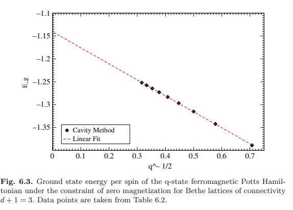
With the order parameters at hand, we can write the energy per link directly using (6.20). For the energy per node, unfortunately, we cannot write a simple expression for all numbers of parts $q$ and have to calculate $\Delta E_1$ by using Monte Carlo methods. It is interesting to study the ground state energy and modularity as a function of the number of parts $q$. Naturally, the absolute value of the ground state energy decreases as we divide the random lattice into more and more parts. However, when looking at the modularity, we see that the term $1 / q$ which we have to subtract from the negative value of the energy in (6.3) decreases for larger numbers of $Q$. Plotting $E_{g s}$ vs. $q^{-1 / 2}$ in Fig. 6.3 we observe a linear dependence which together with (6.3) suggests the existence of an optimal number of $q$ which maximizes the modularity $Q_q$. Empirically, we find by fitting our data
$$
E_g(q)=E_{\infty}-\frac{B}{\sqrt{q}},
$$
with $E_{\infty}=-1.141$ and $B=0.3496$. This is a remarkable result as it shows that even for large numbers of $q$ we can still satisfy 2.3 of the 3 connections per node on average. This is not much less than the 2.78 links per node which can be satisfied when partitioning in only two parts. This also means that practically every node has two or more links into its own community, which again means that every random Bethe lattice of connectivity $d+1=3$ has a community structure if the definitions of Radicchi et al. are applied. Plugging (6.45) into (6.3) we can find the number of parts which maximizes $Q_q$ as
$$
q^*=\frac{k^2}{B^2} \approx 74 .
$$

数学代写|复杂网络代写complex networks代考|NIT1104

数学代写|复杂网络代写complex networks代考|Limit of Dense Graphs with Poissonian Degree Distribution

泊松度分布的特殊形式迄今已导致了许多简化。两个重要的简化是消去了$\left(n_0+2 n\right)$ !它解耦了(6.28)中的和,并且对于这个分布,度分布和多余度分布确实是相同的,这简化了(6.33)中每个节点能量的计算。

这些简化使我们能够研究大平均度极限下泊松图双分划问题的基态能量的标度问题。我们将表明,这使我们能够恢复Fu和Anderson[15]的副本计算结果加上校正项。(6.28)中的贝塞尔函数可以近似为大参数$x \gg n$和固定的$n$ as
$$
I_1(n, x) \approx \frac{e^x}{\sqrt{2 \pi x}}
$$
利用这个近似,我们可以得到阶参量$\eta_1$的下式:
$$
2 \eta_1 \approx 1-\left(4 \pi \lambda \eta_1\right)^{-1 / 2} .
$$
式(6.35)用式(6.38)和式(6.39)近似表示
$$
X_\lambda \approx \frac{1}{2} \sqrt{\frac{1}{\pi \lambda}} \sqrt{\eta_1}=\eta_1-2 \eta_1^2 .
$$
现在我们将(6.39)的解展开为$1 / \lambda$的幂,从而得到$\eta_1$的近似值,因此得到$\eta_1^2$ as
$$
\begin{aligned}
\eta_1 & \approx \frac{1}{2}-\frac{1}{4} \sqrt{\frac{2}{\pi \lambda}}-\frac{1}{8 \pi \lambda}+\mathcal{O}\left(\lambda^{-3 / 2}\right) \text { and } \
\eta_1^2 & \approx \frac{1}{4}-\frac{1}{4} \sqrt{\frac{2}{\pi \lambda}}+\mathcal{O}\left(\lambda^{-3 / 2}\right) .
\end{aligned}
$$

数学代写|复杂网络代写complex networks代考|q-Partitioning of a Bethe Lattice with three Links per Node

到目前为止,我们已经处理了任意度分布图的双分区,作为我们可以将场方程写成耦合多项式系统的一种情况。另一种特殊情况是贝特格,每个节点都有$k=3$个邻居。然后,每条边都指向一个具有多余度$d=2$的节点,我们可以将阶参数$\eta_\tau$写成如下公式:
$$
\begin{aligned}
\eta_\tau= & \sum_{\alpha=1}^{\tau-1}\left(\begin{array}{c}
\tau \
\alpha
\end{array}\right) \eta_\alpha \eta_{\tau-\alpha}+\eta_\tau^2+2 \eta_\tau \sum_{\alpha=1}^{q-\tau}\left(\begin{array}{c}
q-\tau \
\alpha
\end{array}\right) \eta_{\tau+\alpha} \
& +\sum_{\alpha=1}^{q-\tau} \sum_{\beta=1}^{q-\tau-\alpha}\left(\begin{array}{c}
q-\tau \
\alpha
\end{array}\right)\left(\begin{array}{c}
q-\tau-\alpha \
\beta
\end{array}\right) \eta_{\tau+\alpha} \eta_{\tau+\beta} .
\end{aligned}
$$
这很容易解释。包含$\tau$非零条目的消息可以通过组合两个消息来形成,一个包含$\alpha<\tau$,另一个包含$\tau-\alpha$非零条目,它们不像第一个项那样重叠。然后,两个完全具有$\tau$非零条目的消息可能像第二项一样重叠。第三项表示将一个消息与$\tau$和一个消息与$\alpha>\tau$非零条目组合在一起的可能性,而最后一项表示在组合两个消息时恰好有$\tau$个非零条目重叠的可能性,这两个消息都有超过$\tau$个非零条目。

有了顺序参数,我们可以直接使用式(6.20)写出每个链路的能量。对于每个节点的能量,不幸的是,我们不能写出一个简单的表达式为所有数量的部分$q$,必须通过使用蒙特卡罗方法计算$\Delta E_1$。研究基态能量和模块化作为零件数量的函数$q$是很有趣的。当我们将随机晶格分成越来越多的部分时,基态能量的绝对值自然会减小。然而,当观察模块化时,我们看到,我们必须从(6.3)中的负值中减去的项$1 / q$随着$Q$的数量增加而减少。在图6.3中绘制$E_{g s}$与$q^{-1 / 2}$,我们观察到线性依赖关系,它与(6.3)一起表明存在最优数量$q$,使模块化$Q_q$最大化。根据经验,我们通过拟合我们的数据来发现
$$
E_g(q)=E_{\infty}-\frac{B}{\sqrt{q}},
$$
有$E_{\infty}=-1.141$和$B=0.3496$。这是一个显著的结果,因为它表明,即使对于大量的$q$,我们仍然可以平均满足每个节点3个连接中的2.3个。这并不比每个节点的2.78个链接少多少,如果只划分为两个部分,就可以满足这个要求。这也意味着实际上每个节点都有两个或多个链接到自己的社区,这再次意味着如果应用Radicchi等人的定义,每个连接的随机Bethe格$d+1=3$都有一个社区结构。将(6.45)代入(6.3),我们可以找到使$Q_q$ as最大化的零件数
$$
q^*=\frac{k^2}{B^2} \approx 74 .
$$

统计代写|复杂网络代写complex networks代考 请认准statistics-lab™

统计代写请认准statistics-lab™. statistics-lab™为您的留学生涯保驾护航。统计代写|python代写代考

随机过程代考

在概率论概念中,随机过程随机变量的集合。 若一随机系统的样本点是随机函数,则称此函数为样本函数,这一随机系统全部样本函数的集合是一个随机过程。 实际应用中,样本函数的一般定义在时间域或者空间域。 随机过程的实例如股票和汇率的波动、语音信号、视频信号、体温的变化,随机运动如布朗运动、随机徘徊等等。

贝叶斯方法代考

贝叶斯统计概念及数据分析表示使用概率陈述回答有关未知参数的研究问题以及统计范式。后验分布包括关于参数的先验分布,和基于观测数据提供关于参数的信息似然模型。根据选择的先验分布和似然模型,后验分布可以解析或近似,例如,马尔科夫链蒙特卡罗 (MCMC) 方法之一。贝叶斯统计概念及数据分析使用后验分布来形成模型参数的各种摘要,包括点估计,如后验平均值、中位数、百分位数和称为可信区间的区间估计。此外,所有关于模型参数的统计检验都可以表示为基于估计后验分布的概率报表。

广义线性模型代考

广义线性模型(GLM)归属统计学领域,是一种应用灵活的线性回归模型。该模型允许因变量的偏差分布有除了正态分布之外的其它分布。

statistics-lab作为专业的留学生服务机构,多年来已为美国、英国、加拿大、澳洲等留学热门地的学生提供专业的学术服务,包括但不限于Essay代写,Assignment代写,Dissertation代写,Report代写,小组作业代写,Proposal代写,Paper代写,Presentation代写,计算机作业代写,论文修改和润色,网课代做,exam代考等等。写作范围涵盖高中,本科,研究生等海外留学全阶段,辐射金融,经济学,会计学,审计学,管理学等全球99%专业科目。写作团队既有专业英语母语作者,也有海外名校硕博留学生,每位写作老师都拥有过硬的语言能力,专业的学科背景和学术写作经验。我们承诺100%原创,100%专业,100%准时,100%满意。

机器学习代写

随着AI的大潮到来,Machine Learning逐渐成为一个新的学习热点。同时与传统CS相比,Machine Learning在其他领域也有着广泛的应用,因此这门学科成为不仅折磨CS专业同学的“小恶魔”,也是折磨生物、化学、统计等其他学科留学生的“大魔王”。学习Machine learning的一大绊脚石在于使用语言众多,跨学科范围广,所以学习起来尤其困难。但是不管你在学习Machine Learning时遇到任何难题,StudyGate专业导师团队都能为你轻松解决。

多元统计分析代考


基础数据: $N$ 个样本, $P$ 个变量数的单样本,组成的横列的数据表
变量定性: 分类和顺序;变量定量:数值
数学公式的角度分为: 因变量与自变量

时间序列分析代写

随机过程,是依赖于参数的一组随机变量的全体,参数通常是时间。 随机变量是随机现象的数量表现,其时间序列是一组按照时间发生先后顺序进行排列的数据点序列。通常一组时间序列的时间间隔为一恒定值(如1秒,5分钟,12小时,7天,1年),因此时间序列可以作为离散时间数据进行分析处理。研究时间序列数据的意义在于现实中,往往需要研究某个事物其随时间发展变化的规律。这就需要通过研究该事物过去发展的历史记录,以得到其自身发展的规律。

回归分析代写

多元回归分析渐进(Multiple Regression Analysis Asymptotics)属于计量经济学领域,主要是一种数学上的统计分析方法,可以分析复杂情况下各影响因素的数学关系,在自然科学、社会和经济学等多个领域内应用广泛。

MATLAB代写

MATLAB 是一种用于技术计算的高性能语言。它将计算、可视化和编程集成在一个易于使用的环境中,其中问题和解决方案以熟悉的数学符号表示。典型用途包括:数学和计算算法开发建模、仿真和原型制作数据分析、探索和可视化科学和工程图形应用程序开发,包括图形用户界面构建MATLAB 是一个交互式系统,其基本数据元素是一个不需要维度的数组。这使您可以解决许多技术计算问题,尤其是那些具有矩阵和向量公式的问题,而只需用 C 或 Fortran 等标量非交互式语言编写程序所需的时间的一小部分。MATLAB 名称代表矩阵实验室。MATLAB 最初的编写目的是提供对由 LINPACK 和 EISPACK 项目开发的矩阵软件的轻松访问,这两个项目共同代表了矩阵计算软件的最新技术。MATLAB 经过多年的发展,得到了许多用户的投入。在大学环境中,它是数学、工程和科学入门和高级课程的标准教学工具。在工业领域,MATLAB 是高效研究、开发和分析的首选工具。MATLAB 具有一系列称为工具箱的特定于应用程序的解决方案。对于大多数 MATLAB 用户来说非常重要,工具箱允许您学习应用专业技术。工具箱是 MATLAB 函数(M 文件)的综合集合,可扩展 MATLAB 环境以解决特定类别的问题。可用工具箱的领域包括信号处理、控制系统、神经网络、模糊逻辑、小波、仿真等。

R语言代写问卷设计与分析代写
PYTHON代写回归分析与线性模型代写
MATLAB代写方差分析与试验设计代写
STATA代写机器学习/统计学习代写
SPSS代写计量经济学代写
EVIEWS代写时间序列分析代写
EXCEL代写深度学习代写
SQL代写各种数据建模与可视化代写

数学代写|复杂网络代写complex networks代考|CS7280

如果你也在 怎样代写复杂网络Complex Network 这个学科遇到相关的难题,请随时右上角联系我们的24/7代写客服。复杂网络Complex Network分析研究如何识别、描述、可视化和分析复杂网络。分析网络最突出的方法是使用Python库NetworkX,它为构造和绘制复杂的神经网络提供了一种突出的方法。

复杂网络Complex NetworkCNA研究和应用爆炸式增长的主要原因有两个因素:一是廉价而强大的计算机的可用性,使在数学、物理和社会科学方面受过高级培训的研究人员和科学家能够进行一流的研究;另一个因素是人类社会、行为、生物、金融和技术方面日益复杂。

statistics-lab™ 为您的留学生涯保驾护航 在代写复杂网络complex networks方面已经树立了自己的口碑, 保证靠谱, 高质且原创的统计Statistics代写服务。我们的专家在代写复杂网络complex networks方面经验极为丰富,各种代写复杂网络complex networks相关的作业也就用不着说。

数学代写|复杂网络代写complex networks代考|CS7280

数学代写|复杂网络代写complex networks代考|Benchmarking the Algorithm

In order to benchmark the performance of the Potts model approach to community detection, it is applied to computer-generated test networks. Networks with communities of equal and different size were constructed. Those with equal size had 128 nodes, grouped into 4 communities of size 32 . Those with differently sized communities had 320 nodes, grouped into 4 communities of size $32,64,96$ and 128 . In both types of networks, each node has an average degree of $\langle k\rangle=16$. The average number of links to members of the same community $\left\langle k_{i n}\right\rangle$ and to members of different communities $\left\langle k_{\text {out }}\right\rangle$ is then varied, but always ensuring $\left\langle k_{\text {in }}\right\rangle+\left\langle k_{\text {out }}\right\rangle=\langle k\rangle$. Hence, decreasing $k_{\text {in }}$ renders the problem of community detection more difficult.

Recovering a known community structure, any algorithm has to fulfill two criteria: it has to group nodes in the same community which belong together by design and it has to group nodes apart which belong to different communities by design. The first criterion is called “sensitivity” and measures the percentage of pairs of nodes which are correctly grouped together. The second criterion is called “specificity” and measures the percentage of pairs of nodes which are correctly grouped apart.

Because of the Poisson nature of the degree distribution, a connection model of $p_{i j}=p$ was used. Figure 4.5 shows the result of this experiment in comparison with the results obtained from the algorithm of Girvan and Newman [14]. Clearly, both algorithms show high sensitivity and high specificity. However, the Potts model outperforms the GN algorithm on both types of networks in both sensitivity and specificity. When relaxing the Potts model Hamiltonian from random initial conditions at zero temperature, performance decreases, but is still as good as that of the GN algorithm.

An important aspect is the dependence of the sensitivity (specificity) of the algorithm on the number of allowed spin states $q$. Figure 4.6 shows that as long as $q \geq 4$, i.e., the actual number of communities in the network, the value of $q$ is irrelevant. This result is also independent of the strength of the community structure under investigation, i.e., independent of $k_{i n}$. Furthermore, it is necessary to study the stability of results with respect to a change in $\gamma$. As Fig. 4.6 shows, the better the community structure is defined, i.e., the greater $k_{i n}$ is with respect to $\langle k\rangle$, the more stable are the results. The maxima of the curves for all values of $k_{i n}$, however, coincide at $\gamma=1$, i.e., at the point where the contribution of missing and existing links is equal. The same statements also apply to the specificity.

数学代写|复杂网络代写complex networks代考|Community Detection and Graph Partitioning

In order to assess the statistical significance of the community structures found with any algorithm, it is necessary to compare them with expectation values for random networks. This is of course always possible by rewiring the network randomly [15], keeping the degree distribution invariant and then running a community detection algorithm again, comparing the result to the original network. This method, however, can only give an answer to what a particular community detection algorithm may find in a random network and hence depends on the very method of community detection used. It seems a much better method would be to compare the results of a community detection algorithm with a theoretical result, obtained independently of any algorithm. It was shown in previous sections that the problem of community detection can be mapped onto finding the ground state of an infinite range spin glass. A number of techniques exist to calculate expectation values for the energy and the local field distribution in the ground state of spin glasses, given that the couplings between spins are random, but with a known distribution. In the remainder of this chapter and in the following ones, we will make extensive use of these techniques.

What does the community structure of a completely random network look like? The first observation one makes is that the configuration space or the number of possible assignments into $q$ communities is largest when these groups are equal in size, i.e., contain the same number of nodes $N / q$. One can also show that the variance of the number of links within communities is largest when they are of equal size. These two facts taken together mean that in random networks, the assignment of nodes into communities with maximal modularity will with very high probability lead to equal-sized communities. Hence, we only need to calculate expectation values for the modularity of a partition of the network into equal-sized groups. In the language of spin glasses, this means we are looking for the energy of a ground state with zero magnetization. We can also say that we are looking for a partition into $q$ equal-sized groups with a maximum number of links within groups, or, equivalently, with a minimum number of links between groups. The latter is a standard problem in combinatorial optimization and is known as the graph partitioning problem. In short, the communities which form the partition of maximum modularity in a random network will correspond to a minimum cut equipartition.

数学代写|复杂网络代写complex networks代考|CS7280

数学代写|复杂网络代写complex networks代考|Benchmarking the Algorithm

为了测试Potts模型在社区检测中的性能,将其应用于计算机生成的测试网络。构建了大小不等的社区网络。大小相同的有128个节点,分成4个32个节点的社区。不同大小的群落有320个节点,分为4个群落,大小分别为$32,64,96$和128。在这两种类型的网络中,每个节点的平均度为$\langle k\rangle=16$。到同一社区成员$\left\langle k_{i n}\right\rangle$和不同社区成员$\left\langle k_{\text {out }}\right\rangle$的平均链接数是不同的,但始终确保$\left\langle k_{\text {in }}\right\rangle+\left\langle k_{\text {out }}\right\rangle=\langle k\rangle$。因此,减少$k_{\text {in }}$使得社区检测问题更加困难。

恢复一个已知的社区结构,任何算法都必须满足两个标准:它必须将同一社区中的节点按照设计分组在一起,并且必须将属于不同社区的节点按照设计分组分开。第一个标准被称为“灵敏度”,衡量正确组合在一起的节点对的百分比。第二个标准被称为“特异性”,衡量正确分组的节点对的百分比。

由于度分布的泊松性质,使用$p_{i j}=p$的连接模型。图4.5为本实验结果与Girvan和Newman[14]算法结果的对比。显然,这两种算法都具有高灵敏度和高特异性。然而,Potts模型在两种类型的网络上的敏感性和特异性都优于GN算法。当在零温度下从随机初始条件放宽Potts模型哈密顿量时,性能下降,但仍然与GN算法一样好。

一个重要的方面是该算法的灵敏度(特异性)依赖于允许的自旋态的数量$q$。从图4.6可以看出,只要$q \geq 4$即网络中社区的实际数量,$q$的值就无关紧要。该结果也独立于所调查的社区结构的强度,即独立于$k_{i n}$。此外,有必要研究结果相对于$\gamma$的变化的稳定性。如图4.6所示,群落结构定义得越好,即$k_{i n}$相对于$\langle k\rangle$越大,则结果越稳定。然而,所有$k_{i n}$值的曲线的最大值在$\gamma=1$重合,即在缺失链接和现有链接的贡献相等的点上。同样的陈述也适用于特异性。

数学代写|复杂网络代写complex networks代考|Community Detection and Graph Partitioning

为了评估用任何算法找到的群体结构的统计显著性,有必要将它们与随机网络的期望值进行比较。当然,这总是可以通过随机重新连接网络来实现[15],保持度分布不变,然后再次运行社区检测算法,将结果与原始网络进行比较。然而,这种方法只能给出特定社区检测算法在随机网络中可能发现的答案,因此取决于所使用的社区检测方法。似乎更好的方法是将社区检测算法的结果与独立于任何算法获得的理论结果进行比较。在前面的章节中已经表明,共同体检测的问题可以映射到寻找无限范围自旋玻璃的基态。考虑到自旋玻璃之间的耦合是随机的,但有一个已知的分布,存在许多技术来计算自旋玻璃基态的能量和局部场分布的期望值。在本章的剩余部分和以下几章中,我们将广泛使用这些技术。

一个完全随机网络的社区结构是什么样的?第一个观察结果是,当这些组的大小相等时,配置空间或可能分配到$q$社区的数量最大,即包含相同数量的节点$N / q$。我们还可以证明,当社区内的链接大小相等时,它们的数量差异最大。这两个事实结合在一起意味着,在随机网络中,将节点分配到具有最大模块化的社区将有很大的概率导致等大小的社区。因此,我们只需要计算网络划分为大小相等的组的模块化的期望值。在自旋玻璃的语言中,这意味着我们正在寻找具有零磁化的基态的能量。我们也可以说,我们正在寻找一个划分为$q$大小相等的组,组内具有最大数量的链接,或者,等价地,组之间具有最小数量的链接。后者是组合优化中的一个标准问题,被称为图划分问题。简而言之,在一个随机网络中,组成最大模块划分的社团对应于一个最小切割均分。

统计代写|复杂网络代写complex networks代考 请认准statistics-lab™

统计代写请认准statistics-lab™. statistics-lab™为您的留学生涯保驾护航。统计代写|python代写代考

随机过程代考

在概率论概念中,随机过程随机变量的集合。 若一随机系统的样本点是随机函数,则称此函数为样本函数,这一随机系统全部样本函数的集合是一个随机过程。 实际应用中,样本函数的一般定义在时间域或者空间域。 随机过程的实例如股票和汇率的波动、语音信号、视频信号、体温的变化,随机运动如布朗运动、随机徘徊等等。

贝叶斯方法代考

贝叶斯统计概念及数据分析表示使用概率陈述回答有关未知参数的研究问题以及统计范式。后验分布包括关于参数的先验分布,和基于观测数据提供关于参数的信息似然模型。根据选择的先验分布和似然模型,后验分布可以解析或近似,例如,马尔科夫链蒙特卡罗 (MCMC) 方法之一。贝叶斯统计概念及数据分析使用后验分布来形成模型参数的各种摘要,包括点估计,如后验平均值、中位数、百分位数和称为可信区间的区间估计。此外,所有关于模型参数的统计检验都可以表示为基于估计后验分布的概率报表。

广义线性模型代考

广义线性模型(GLM)归属统计学领域,是一种应用灵活的线性回归模型。该模型允许因变量的偏差分布有除了正态分布之外的其它分布。

statistics-lab作为专业的留学生服务机构,多年来已为美国、英国、加拿大、澳洲等留学热门地的学生提供专业的学术服务,包括但不限于Essay代写,Assignment代写,Dissertation代写,Report代写,小组作业代写,Proposal代写,Paper代写,Presentation代写,计算机作业代写,论文修改和润色,网课代做,exam代考等等。写作范围涵盖高中,本科,研究生等海外留学全阶段,辐射金融,经济学,会计学,审计学,管理学等全球99%专业科目。写作团队既有专业英语母语作者,也有海外名校硕博留学生,每位写作老师都拥有过硬的语言能力,专业的学科背景和学术写作经验。我们承诺100%原创,100%专业,100%准时,100%满意。

机器学习代写

随着AI的大潮到来,Machine Learning逐渐成为一个新的学习热点。同时与传统CS相比,Machine Learning在其他领域也有着广泛的应用,因此这门学科成为不仅折磨CS专业同学的“小恶魔”,也是折磨生物、化学、统计等其他学科留学生的“大魔王”。学习Machine learning的一大绊脚石在于使用语言众多,跨学科范围广,所以学习起来尤其困难。但是不管你在学习Machine Learning时遇到任何难题,StudyGate专业导师团队都能为你轻松解决。

多元统计分析代考


基础数据: $N$ 个样本, $P$ 个变量数的单样本,组成的横列的数据表
变量定性: 分类和顺序;变量定量:数值
数学公式的角度分为: 因变量与自变量

时间序列分析代写

随机过程,是依赖于参数的一组随机变量的全体,参数通常是时间。 随机变量是随机现象的数量表现,其时间序列是一组按照时间发生先后顺序进行排列的数据点序列。通常一组时间序列的时间间隔为一恒定值(如1秒,5分钟,12小时,7天,1年),因此时间序列可以作为离散时间数据进行分析处理。研究时间序列数据的意义在于现实中,往往需要研究某个事物其随时间发展变化的规律。这就需要通过研究该事物过去发展的历史记录,以得到其自身发展的规律。

回归分析代写

多元回归分析渐进(Multiple Regression Analysis Asymptotics)属于计量经济学领域,主要是一种数学上的统计分析方法,可以分析复杂情况下各影响因素的数学关系,在自然科学、社会和经济学等多个领域内应用广泛。

MATLAB代写

MATLAB 是一种用于技术计算的高性能语言。它将计算、可视化和编程集成在一个易于使用的环境中,其中问题和解决方案以熟悉的数学符号表示。典型用途包括:数学和计算算法开发建模、仿真和原型制作数据分析、探索和可视化科学和工程图形应用程序开发,包括图形用户界面构建MATLAB 是一个交互式系统,其基本数据元素是一个不需要维度的数组。这使您可以解决许多技术计算问题,尤其是那些具有矩阵和向量公式的问题,而只需用 C 或 Fortran 等标量非交互式语言编写程序所需的时间的一小部分。MATLAB 名称代表矩阵实验室。MATLAB 最初的编写目的是提供对由 LINPACK 和 EISPACK 项目开发的矩阵软件的轻松访问,这两个项目共同代表了矩阵计算软件的最新技术。MATLAB 经过多年的发展,得到了许多用户的投入。在大学环境中,它是数学、工程和科学入门和高级课程的标准教学工具。在工业领域,MATLAB 是高效研究、开发和分析的首选工具。MATLAB 具有一系列称为工具箱的特定于应用程序的解决方案。对于大多数 MATLAB 用户来说非常重要,工具箱允许您学习应用专业技术。工具箱是 MATLAB 函数(M 文件)的综合集合,可扩展 MATLAB 环境以解决特定类别的问题。可用工具箱的领域包括信号处理、控制系统、神经网络、模糊逻辑、小波、仿真等。

R语言代写问卷设计与分析代写
PYTHON代写回归分析与线性模型代写
MATLAB代写方差分析与试验设计代写
STATA代写机器学习/统计学习代写
SPSS代写计量经济学代写
EVIEWS代写时间序列分析代写
EXCEL代写深度学习代写
SQL代写各种数据建模与可视化代写

统计代写|复杂网络代写complex networks代考|CS60078

如果你也在 怎样代写复杂网络Complex Network 这个学科遇到相关的难题,请随时右上角联系我们的24/7代写客服。复杂网络Complex Network分析研究如何识别、描述、可视化和分析复杂网络。分析网络最突出的方法是使用Python库NetworkX,它为构造和绘制复杂的神经网络提供了一种突出的方法。

复杂网络Complex NetworkCNA研究和应用爆炸式增长的主要原因有两个因素:一是廉价而强大的计算机的可用性,使在数学、物理和社会科学方面受过高级培训的研究人员和科学家能够进行一流的研究;另一个因素是人类社会、行为、生物、金融和技术方面日益复杂。

statistics-lab™ 为您的留学生涯保驾护航 在代写复杂网络complex networks方面已经树立了自己的口碑, 保证靠谱, 高质且原创的统计Statistics代写服务。我们的专家在代写复杂网络complex networks方面经验极为丰富,各种代写复杂网络complex networks相关的作业也就用不着说。

统计代写|复杂网络代写complex networks代考|CS60078

统计代写|复杂网络代写complex networks代考|Non-hierarchical

The non-hierarchical methods approach the problem from a different perspective. In principle, they intend to calculate a full distance matrix for the nodes of the network. This can then be treated by conventional techniques.

One of the earliest approaches to community detection is due to Eriksen et al. $[41,42]$. They study a diffusion process on a network and analyze the decay of the modes of the following diffusive system with discrete time:

$$
\rho_i(t+1)-\rho_i(t)=\sum_j\left(T_{i j}-\delta_{i j}\right) \rho_j(t) .
$$
Here $T_{i j}$ represents the adjacency matrix of the network such that $T_{i j}=1 / k_j$ for $A_{i j}=1$ and zero otherwise. Hence $T_{i j}$ represents the probability of a random walker to go from $j$ to $i$. The decay of a random initial configuration $\rho(t=0)$ toward the steady state is characterized by the eigenmodes of the transition matrix $T_{i j}$. The eigenvectors corresponding to the largest eigenvalues can then be used to define a distance between nodes which helps in identifying communities. To do this, the eigenvectors belonging to the largest non-trivial positive eigenvalues are plotted against each other. This diffusion approach is very similar in spirit to other algorithms based on the idea of using flow simulations for community detection as suggested by van Dongen [43] under the name of “Markov clustering” (MCL).

The method presented by Zhou [44-46] first converts the sparse adjacency matrix of the graph into a full distance matrix by calculating the average time a Brownian particle needs to move from node $i$ to $j$. Then this distance matrix is clustered using ordinary hierarchical clustering algorithms. This approach is based on the observation that a random walker has shorter traveling time between two nodes if many (short) alternative paths exist.

Another spectral approach has been taken by Muños and Donetti [47]. They work with the Laplacian matrix of the network. The Laplacian is defined as
$$
L_{i j}=k_i \delta_{i j}-A_{i j} .
$$

统计代写|复杂网络代写complex networks代考|Optimization Based

A different approach which is reminiscent of the parametric clustering procedures known in computer science is the idea of searching for partitions with maximum modularity $Q$ using combinatorial optimization techniques [48]. This approach has been adopted by Guimera et al. in Refs. [2, 49] or Massen et al. [50] using simulated annealing [51] or Duch and Arenas using extremal optimization [52].

Though this approach will be the preferred one for the remainder of this book, a number of issues remain. For the hierarchical algorithms, a community was to be understood as whatever the algorithm outputs. Now, it is not the algorithm that defines what a community is, but the quality function, i.e., the modularity $Q$ in this case. Also, the modularity $Q$ as defined by Newman $[23]$ is parameter free and an understanding for hierarchical and overlapping structures needs to be developed.

Block structure in networks is a very common and well-studied phenomenon. The concepts of structural and regular equivalence as well as the types of blocks defined for generalized block modeling are well defined but appear too rigid to be of practical use for large and noisy data sets. Diagonal block models or modular structures have received particular attention in the literature and have developed into an almost independent concept of cohesive subgroups or communities. The comparison of many different community definitions from various fields has shown that the concept of module or community in a network is only vaguely defined. The diversity of algorithms published is only a consequence of this vague definition. None of the algorithms could be called “ideal” in the sense that it combines the features of computational efficiency, accuracy, flexibility and adaptability with regard to the network and easy interpretation of the results. More importantly, none of the above-cited publications allows an estimation to which degree the community structure found is a reality of the network or a product of the clustering process itself. The following chapters are addressing these issues and present a framework in which community detection is viewed again as a special case of a general procedure for detecting block structure in networks.

统计代写|复杂网络代写complex networks代考|CS60078

复杂网络代写

统计代写|复杂网络代写complex networks代考|Non-hierarchical

非分层方法从不同的角度处理问题。原则上,他们打算计算网络节点的全距离矩阵。然后可以用常规技术来处理。

最早的社区检测方法之一来自Eriksen等人$[41,42]$。他们研究了网络上的扩散过程,并分析了以下扩散系统的模态随离散时间的衰减:

$$
\rho_i(t+1)-\rho_i(t)=\sum_j\left(T_{i j}-\delta_{i j}\right) \rho_j(t) .
$$
这里$T_{i j}$表示网络的邻接矩阵,使得$A_{i j}=1$为$T_{i j}=1 / k_j$,否则为零。因此$T_{i j}$表示随机步行者从$j$到$i$的概率。随机初始构型$\rho(t=0)$向稳态的衰减由跃迁矩阵$T_{i j}$的特征模态表征。与最大特征值相对应的特征向量可以用来定义节点之间的距离,这有助于识别社区。为了做到这一点,属于最大非平凡正特征值的特征向量被相互绘制。这种扩散方法在精神上与van Dongen[43]以“马尔可夫聚类”(Markov clustering, MCL)的名义提出的基于使用流模拟进行社区检测的思想的其他算法非常相似。

Zhou[44-46]提出的方法首先通过计算布朗粒子从节点$i$移动到$j$所需的平均时间,将图的稀疏邻接矩阵转换为全距离矩阵。然后使用普通的层次聚类算法对该距离矩阵进行聚类。这种方法是基于这样的观察:如果存在许多(短)可选路径,则随机行走器在两个节点之间的行走时间会更短。

Muños和Donetti[47]采用了另一种光谱方法。他们使用网络的拉普拉斯矩阵。拉普拉斯式定义为
$$
L_{i j}=k_i \delta_{i j}-A_{i j} .
$$

统计代写|复杂网络代写complex networks代考|Optimization Based

另一种与计算机科学中已知的参数聚类过程类似的方法是使用组合优化技术搜索具有最大模块化$Q$的分区[48]。Guimera等人在参考文献中采用了这种方法。[2,49]或Massen等[50]使用模拟退火[51]或Duch和Arenas使用极值优化[52]。

尽管这种方法将是本书其余部分的首选方法,但仍然存在一些问题。对于分层算法,社区被理解为算法的输出。现在,定义社区的不是算法,而是质量函数,即本例中的模块化Q。此外,Newman $[23]定义的模块化$Q$是无参数的,需要发展对分层和重叠结构的理解。

网络中的块结构是一种非常普遍且被充分研究的现象。结构等价和规则等价的概念以及为广义块建模定义的块的类型都有很好的定义,但对于大型和有噪声的数据集来说,似乎过于严格而无法实际使用。对角块模型或模块化结构在文献中受到了特别的关注,并已发展成为一个几乎独立的凝聚力子群体或社区的概念。通过比较不同领域对社区的定义,可以发现网络中模块或社区的定义是模糊的。发表的算法的多样性只是这种模糊定义的结果。没有一种算法可以被称为“理想”,因为它结合了计算效率、准确性、灵活性和网络适应性以及易于解释结果的特点。更重要的是,上述引用的出版物都不允许估计发现的社区结构在多大程度上是网络的现实或聚类过程本身的产物。下面的章节将讨论这些问题,并提出一个框架,在这个框架中,社区检测再次被视为检测网络中块结构的一般程序的特殊情况。

统计代写|复杂网络代写complex networks代考 请认准statistics-lab™

统计代写请认准statistics-lab™. statistics-lab™为您的留学生涯保驾护航。统计代写|python代写代考

随机过程代考

在概率论概念中,随机过程随机变量的集合。 若一随机系统的样本点是随机函数,则称此函数为样本函数,这一随机系统全部样本函数的集合是一个随机过程。 实际应用中,样本函数的一般定义在时间域或者空间域。 随机过程的实例如股票和汇率的波动、语音信号、视频信号、体温的变化,随机运动如布朗运动、随机徘徊等等。

贝叶斯方法代考

贝叶斯统计概念及数据分析表示使用概率陈述回答有关未知参数的研究问题以及统计范式。后验分布包括关于参数的先验分布,和基于观测数据提供关于参数的信息似然模型。根据选择的先验分布和似然模型,后验分布可以解析或近似,例如,马尔科夫链蒙特卡罗 (MCMC) 方法之一。贝叶斯统计概念及数据分析使用后验分布来形成模型参数的各种摘要,包括点估计,如后验平均值、中位数、百分位数和称为可信区间的区间估计。此外,所有关于模型参数的统计检验都可以表示为基于估计后验分布的概率报表。

广义线性模型代考

广义线性模型(GLM)归属统计学领域,是一种应用灵活的线性回归模型。该模型允许因变量的偏差分布有除了正态分布之外的其它分布。

statistics-lab作为专业的留学生服务机构,多年来已为美国、英国、加拿大、澳洲等留学热门地的学生提供专业的学术服务,包括但不限于Essay代写,Assignment代写,Dissertation代写,Report代写,小组作业代写,Proposal代写,Paper代写,Presentation代写,计算机作业代写,论文修改和润色,网课代做,exam代考等等。写作范围涵盖高中,本科,研究生等海外留学全阶段,辐射金融,经济学,会计学,审计学,管理学等全球99%专业科目。写作团队既有专业英语母语作者,也有海外名校硕博留学生,每位写作老师都拥有过硬的语言能力,专业的学科背景和学术写作经验。我们承诺100%原创,100%专业,100%准时,100%满意。

机器学习代写

随着AI的大潮到来,Machine Learning逐渐成为一个新的学习热点。同时与传统CS相比,Machine Learning在其他领域也有着广泛的应用,因此这门学科成为不仅折磨CS专业同学的“小恶魔”,也是折磨生物、化学、统计等其他学科留学生的“大魔王”。学习Machine learning的一大绊脚石在于使用语言众多,跨学科范围广,所以学习起来尤其困难。但是不管你在学习Machine Learning时遇到任何难题,StudyGate专业导师团队都能为你轻松解决。

多元统计分析代考


基础数据: $N$ 个样本, $P$ 个变量数的单样本,组成的横列的数据表
变量定性: 分类和顺序;变量定量:数值
数学公式的角度分为: 因变量与自变量

时间序列分析代写

随机过程,是依赖于参数的一组随机变量的全体,参数通常是时间。 随机变量是随机现象的数量表现,其时间序列是一组按照时间发生先后顺序进行排列的数据点序列。通常一组时间序列的时间间隔为一恒定值(如1秒,5分钟,12小时,7天,1年),因此时间序列可以作为离散时间数据进行分析处理。研究时间序列数据的意义在于现实中,往往需要研究某个事物其随时间发展变化的规律。这就需要通过研究该事物过去发展的历史记录,以得到其自身发展的规律。

回归分析代写

多元回归分析渐进(Multiple Regression Analysis Asymptotics)属于计量经济学领域,主要是一种数学上的统计分析方法,可以分析复杂情况下各影响因素的数学关系,在自然科学、社会和经济学等多个领域内应用广泛。

MATLAB代写

MATLAB 是一种用于技术计算的高性能语言。它将计算、可视化和编程集成在一个易于使用的环境中,其中问题和解决方案以熟悉的数学符号表示。典型用途包括:数学和计算算法开发建模、仿真和原型制作数据分析、探索和可视化科学和工程图形应用程序开发,包括图形用户界面构建MATLAB 是一个交互式系统,其基本数据元素是一个不需要维度的数组。这使您可以解决许多技术计算问题,尤其是那些具有矩阵和向量公式的问题,而只需用 C 或 Fortran 等标量非交互式语言编写程序所需的时间的一小部分。MATLAB 名称代表矩阵实验室。MATLAB 最初的编写目的是提供对由 LINPACK 和 EISPACK 项目开发的矩阵软件的轻松访问,这两个项目共同代表了矩阵计算软件的最新技术。MATLAB 经过多年的发展,得到了许多用户的投入。在大学环境中,它是数学、工程和科学入门和高级课程的标准教学工具。在工业领域,MATLAB 是高效研究、开发和分析的首选工具。MATLAB 具有一系列称为工具箱的特定于应用程序的解决方案。对于大多数 MATLAB 用户来说非常重要,工具箱允许您学习应用专业技术。工具箱是 MATLAB 函数(M 文件)的综合集合,可扩展 MATLAB 环境以解决特定类别的问题。可用工具箱的领域包括信号处理、控制系统、神经网络、模糊逻辑、小波、仿真等。

R语言代写问卷设计与分析代写
PYTHON代写回归分析与线性模型代写
MATLAB代写方差分析与试验设计代写
STATA代写机器学习/统计学习代写
SPSS代写计量经济学代写
EVIEWS代写时间序列分析代写
EXCEL代写深度学习代写
SQL代写各种数据建模与可视化代写

统计代写|复杂网络代写complex networks代考| Optimizing the Quality Function

如果你也在 怎样代写复杂网络complex networks这个学科遇到相关的难题,请随时右上角联系我们的24/7代写客服。

复杂网络是由数量巨大的节点和节点之间错综复杂的关系共同构成的网络结构。

statistics-lab™ 为您的留学生涯保驾护航 在代写复杂网络complex networks方面已经树立了自己的口碑, 保证靠谱, 高质且原创的统计Statistics代写服务。我们的专家在代写复杂网络complex networks方面经验极为丰富,各种代写复杂网络complex networks相关的作业也就用不着说。

我们提供的复杂网络complex networks及其相关学科的代写,服务范围广, 其中包括但不限于:

  • Statistical Inference 统计推断
  • Statistical Computing 统计计算
  • Advanced Probability Theory 高等楖率论
  • Advanced Mathematical Statistics 高等数理统计学
  • (Generalized) Linear Models 广义线性模型
  • Statistical Machine Learning 统计机器学习
  • Longitudinal Data Analysis 纵向数据分析
  • Foundations of Data Science 数据科学基础
统计代写|复杂网络代写complex networks代考| Optimizing the Quality Function

统计代写|复杂网络代写complex networks代考|Optimizing the Quality Function

After having studied some properties of the configurations and image graphs that optimize (3.13), (3.14) or (3.15), let us now turn to the problem of actually finding these configurations. Though any optimization scheme that can deal with combinatorial optimization problems may be implemented $[8,9]$, the

use of simulated annealing $[10]$ for a Potts model [11] is shown, because it yields high-quality results, is very general in its application and very simple to program. We interpret our quality function $Q$ to be maximized as the negative of a Hamiltonian to be minimized, i.e., we write $\mathcal{H}({\sigma})=-Q$. The single site heat bath update rule at temperature $T=1 / \beta$ then reads as follows:
$$
p\left(\sigma_{i}=\alpha\right)=\frac{\exp \left(-\beta \mathcal{H}\left(\left{\sigma_{j \neq i}, \sigma_{i}=\alpha\right}\right)\right)}{\sum_{s=1}^{q} \exp \left(-\beta \mathcal{H}\left(\left{\sigma_{j \neq i}, \sigma_{i}=s\right}\right)\right)}
$$
That is, the probability of node $i$ being in group $\alpha$ is proportional to the exponential of the energy (negative quality) of the entire system with all other nodes $j \neq i$ fixed and node $i$ in state $\alpha$. Since this is costly to evaluate, one pretends to know the energy of the system with node $i$ in some arbitrarily chosen group $\phi$, which is denoted by $\mathcal{H}{\phi}$. Then one can calculate the energy of the system with $i$ in group $\alpha$ as $\mathcal{H}{\phi}+\Delta \mathcal{H}\left(\sigma_{i}=\phi \rightarrow \alpha\right)$. The energy $\mathcal{H}{\phi}$ then factors out in (3.25) and one is left with $$ p\left(\sigma{i}=\alpha\right)=\frac{\exp \left{-\beta \Delta \mathcal{H}\left(\sigma_{i}=\phi \rightarrow \alpha\right)\right}}{\sum_{s=1}^{q} \exp \left{-\beta \Delta \mathcal{H}\left(\sigma_{i}=\phi \rightarrow s\right)\right}}
$$
Suppose we are trying to fit a network to a given image graph, i.e., $\mathbf{B}$ is given. Then the change in energy $\Delta \mathcal{F} C\left(\sigma_{i}=\phi \rightarrow \alpha\right)$ is easily calculated from the change in quality according to (3.13):
$$
\begin{aligned}
\Delta \mathcal{H}\left(\sigma_{i}=\phi \rightarrow \alpha\right)=& \sum_{s}\left(B_{\phi s}-B_{\alpha s}\right)\left(k_{i \rightarrow s}^{\text {out }}-\gamma\left[k_{i \rightarrow s}^{\text {out }}\right]\right) \
&+\sum_{r}\left(B_{r \phi}-B_{r \alpha}\right)\left(k_{r \rightarrow i}^{i n}-\gamma\left[k_{r \rightarrow i}^{i n}\right]\right) \
=& \sum_{s}\left(B_{\phi s}-B_{\alpha s}\right) a_{i s}+\sum_{r}\left(B_{r \phi}-B_{r \alpha}\right) a_{r i}
\end{aligned}
$$

统计代写|复杂网络代写complex networks代考|Properties of the Ground State

From the fact that the ground state is a configuration which is a minimum in the configuration space, one can derive a number of properties of the communities that apply to any local minimum of the Hamiltonian in the configuration space. If one takes these properties as defining properties of what a community is, one then finds valid alternative community structures also in the local minima of the Hamiltonian. The energies of these local minima will then allow us to compare these community structures. It may be that alternative

but almost equally “good” community structures exist. Before proceeding to investigate the properties of spin configurations that represent local minima of the Hamiltonian, a few properties of (4.3) as such shall be discussed:

First, note that for $\gamma=1(4.3)$ evaluates to zero in case of assigning all nodes into the same spin state due to the normalization constraint on $p_{i j}$, i.e., $\sum_{i j} p_{i j}=\sum_{i j} A_{i j}=M$, independent of the graph. Second, for a complete graph, any spin configuration yields the same zero energy at $\gamma=1$. Third, for a graph without edges, e.g., only a set of nodes, any spin configuration gives zero energy independent of $\gamma$. Fourth, the expectation value of (4.3) for a random assignment of spins at $\gamma=1$ is zero. These considerations provide an intuitive feeling for the fact that the lower the energy the better the fit of the diagonal block model to the network and that the choice of $\gamma=1$ will result in what could be called “natural partitioning” of the graph into modules.
Let us consider the case of undirected networks which is most often found in applications. Then, the adjacency matrix of the network is symmetric and we have $k_{i}^{\text {in }}=k_{i}^{\text {out }}$ and thus the coefficients of adhesion are also symmetric, i.e., $a_{r s}=a_{s r}$. According to (3.28) the change in energy to move a group of nodes $n_{1}$ from group $s$ to spin state $r$ is
$$
\Delta \mathcal{H}=a_{1, s \backslash 1}-a_{1 r}
$$
Here $a_{1, s \backslash 1}$ is the adhesion of $n_{1}$ with its complement in group $s$ and $a_{1 r}$ is the adhesion of $n_{1}$ with $n_{r}$. It is clear that if one moves $n_{1}$ to a previously unpopulated spin state, then $\Delta \mathcal{H}=a_{1, s \backslash 1}$. This move corresponds to dividing group $n_{s}$. Furthermore, if $n_{1}=n_{s}$, one has $\Delta \mathcal{H}=-a_{s r}$, which corresponds to joining groups $n_{s}$ and $n_{r}$. A spin configuration can only be a local minimum of the Hamiltonian if a move of this type does not lead to a lower energy. It is clear that some moves may not change the energy and are hence called neutral moves. In cases of equality $a_{1, s \backslash 1}=a_{1, r}$ and $n_{r}$ being a community itself, communities $n_{s}$ and $n_{r}$ are said to have an overlap of the nodes in $n_{1}$.

统计代写|复杂网络代写complex networks代考|Simple Divisive and Agglomerative Approaches

The equivalence of modularity with a spin glass energy shows that the problem of maximizing modularity falls into the class of NP-hard optimization problems [3]. For these problems, it is believed that no algorithm exists that is able to produce an optimal solution in a time that grows only polynomial with the size of the problem instance. However, heuristics such as simulated annealing exist, which are able to find possibly very good solutions. In this section, we will discuss an often used approach to clustering, namely hierarchical agglomerative and divisive algorithms and investigate whether they too are good heuristics for finding partitions of maximum modularity.

A number of community detection algorithms presented in Chap. 2 have followed recursive approaches and lead to hierarchical community structures. Hierarchical clustering techniques can be dichotomized into divisive

and agglomerative approaches [4]. It will be shown how a simple recursive divisive approach and an agglomerative approach may be implemented and where they fail.

In the present framework, a hierarchical divisive algorithm would mean to construct the ground state of the q-state Potts model by recursively partitioning the network into two parts according to the ground state of a 2-state Potts or Ising system. This procedure would be computationally simple and result directly in a hierarchy of clusters due to the recursion of the procedure on the parts until the total energy cannot be lowered anymore. Such a procedure would be justified, if the ground state of the q-state Potts Hamiltonian and the repeated application of the Ising system cut the network along the same edges. Let us derive a condition under which this could be ensured.

In order for this recursive approach to work, one must ensure that the ground state of the 2-state Hamiltonian never cuts though a community as defined by the q-state Hamiltonian. Assume a network made of three communities $n_{1}, n_{2}$ and $n_{3}$ as defined by the ground state of the q-state Hamiltonian. For the bi-partitioning, one now has two possible scenarios. Without loss of generality, the cut is made either between $n_{2}$ and $n_{1}+n_{3}$ or between $n_{1}, n_{2}$ and $n_{3}=n_{a}+n_{b}$, parting the network into $n_{1}+n_{a}$ and $n_{2}+n_{b}$. Since the former situation should be energetically lower for the recursive algorithm to work, one arrives at the condition that
$$
m_{a b}-\left[m_{a b}\right]{p{i j}}+m_{1 b}-\left[m_{1 b}\right]{p{i j}}>m_{2 b}-\left[m_{2 b}\right]{p{i j}}
$$

统计代写|复杂网络代写complex networks代考| Optimizing the Quality Function

复杂网络代写

统计代写|复杂网络代写complex networks代考|Optimizing the Quality Function

在研究了优化 (3.13)、(3.14) 或 (3.15) 的配置和图像图的一些属性之后,现在让我们转向实际找到这些配置的问题。尽管可以实现任何可以处理组合优化问题的优化方案[8,9], 这

使用模拟退火[10]显示了 Potts 模型 [11],因为它产生了高质量的结果,在其应用中非常通用并且编程非常简单。我们解释我们的质量功能问最大化作为要最小化的哈密顿量的负数,即,我们写H(σ)=−问. 温度下的单点热浴更新规则吨=1/b然后内容如下:
p\left(\sigma_{i}=\alpha\right)=\frac{\exp \left(-\beta \mathcal{H}\left(\left{\sigma_{j \neq i}, \sigma_{ i}=\alpha\right}\right)\right)}{\sum_{s=1}^{q} \exp \left(-\beta \mathcal{H}\left(\left{\sigma_{j \neq i}, \sigma_{i}=s\right}\right)\right)}p\left(\sigma_{i}=\alpha\right)=\frac{\exp \left(-\beta \mathcal{H}\left(\left{\sigma_{j \neq i}, \sigma_{ i}=\alpha\right}\right)\right)}{\sum_{s=1}^{q} \exp \left(-\beta \mathcal{H}\left(\left{\sigma_{j \neq i}, \sigma_{i}=s\right}\right)\right)}
即节点的概率一世在群里一种与整个系统与所有其他节点的能量(负质量)指数成正比j≠一世固定和节点一世处于状态一种. 由于评估成本很高,因此假装知道具有节点的系统的能量一世在某个任意选择的组中φ,表示为Hφ. 然后可以计算系统的能量一世在小组中一种作为Hφ+ΔH(σ一世=φ→一种). 能量Hφ然后将(3.25)中的因素排除在外,剩下一个p\left(\sigma{i}=\alpha\right)=\frac{\exp \left{-\beta \Delta \mathcal{H}\left(\sigma_{i}=\phi \rightarrow \alpha\右)\right}}{\sum_{s=1}^{q} \exp \left{-\beta \Delta \mathcal{H}\left(\sigma_{i}=\phi \rightarrow s\right) \对}}p\left(\sigma{i}=\alpha\right)=\frac{\exp \left{-\beta \Delta \mathcal{H}\left(\sigma_{i}=\phi \rightarrow \alpha\右)\right}}{\sum_{s=1}^{q} \exp \left{-\beta \Delta \mathcal{H}\left(\sigma_{i}=\phi \rightarrow s\right) \对}}
假设我们试图将网络拟合到给定的图像图上,即乙给出。然后是能量变化ΔFC(σ一世=φ→一种)很容易根据 (3.13) 从质量变化计算:
ΔH(σ一世=φ→一种)=∑s(乙φs−乙一种s)(ķ一世→s出去 −C[ķ一世→s出去 ]) +∑r(乙rφ−乙r一种)(ķr→一世一世n−C[ķr→一世一世n]) =∑s(乙φs−乙一种s)一种一世s+∑r(乙rφ−乙r一种)一种r一世

统计代写|复杂网络代写complex networks代考|Properties of the Ground State

从基态是配置空间中的最小值的配置这一事实,可以推导出社区的许多属性,这些属性适用于配置空间中哈密顿量的任何局部最小值。如果将这些属性作为社区的定义属性,那么人们也会在哈密顿量的局部最小值中找到有效的替代社区结构。这些局部最小值的能量将使我们能够比较这些社区结构。这可能是另一种选择

但几乎同样“好”的社区结构也存在。在继续研究代表哈密顿量局部最小值的自旋配置的性质之前,应讨论(4.3)的一些性质:

首先,注意对于C=1(4.3)如果由于归一化约束将所有节点分配到相同的自旋状态,则计算为零p一世j, IE,∑一世jp一世j=∑一世j一种一世j=米,独立于图。其次,对于一个完整的图形,任何自旋配置在C=1. 第三,对于没有边的图,例如,只有一组节点,任何自旋配置都给出零能量,独立于C. 第四,(4.3)的期望值对于随机分配的自旋C=1为零。这些考虑提供了一个直观的感觉,即能量越低,对角块模型对网络的拟合越好,并且选择C=1将导致图的“自然分区”成模块。
让我们考虑在应用程序中最常见的无向网络的情况。然后,网络的邻接矩阵是对称的,我们有ķ一世在 =ķ一世出去 因此粘附系数也是对称的,即一种rs=一种sr. 根据(3.28)的能量变化来移动一组节点n1来自组s旋转状态r是
ΔH=一种1,s∖1−一种1r
这里一种1,s∖1是附着力n1及其在组中的补充s和一种1r是附着力n1和nr. 很明显,如果一个人移动n1到以前未填充的自旋状态,然后ΔH=一种1,s∖1. 此招对应分组ns. 此外,如果n1=ns, 一个有ΔH=−一种sr,对应于加入组ns和nr. 如果这种类型的移动不会导致较低的能量,则自旋配置只能是哈密顿量的局部最小值。很明显,有些动作可能不会改变能量,因此被称为中性动作。在平等的情况下一种1,s∖1=一种1,r和nr作为一个社区本身,社区ns和nr据说节点有重叠n1.

统计代写|复杂网络代写complex networks代考|Simple Divisive and Agglomerative Approaches

模块化与自旋玻璃能量的等价性表明,最大化模块化的问题属于 NP-hard 优化问题 [3]。对于这些问题,相信不存在能够在仅随问题实例的大小呈多项式增长的时间内产生最优解的算法。但是,存在诸如模拟退火之类的启发式方法,它们能够找到可能非常好的解决方案。在本节中,我们将讨论一种常用的聚类方法,即分层凝聚和分裂算法,并研究它们是否也是寻找最大模块化分区的良好启发式方法。

第 1 章中介绍了一些社区检测算法。2遵循递归方法并导致分层社区结构。层次聚类技术可以分为分裂的

和凝聚方法[4]。它将展示如何实现简单的递归分裂方法和凝聚方法以及它们失败的地方。

在目前的框架中,层次划分算法意味着通过根据 2 态 Potts 或 Ising 系统的基态将网络递归地划分为两部分来构建 q 态 Potts 模型的基态。这个过程在计算上很简单,并且由于部件上的过程递归直到总能量不能再降低,直接导致集群的层次结构。如果 q-state Potts Hamiltonian 的基态和 Ising 系统的重复应用沿着相同的边缘切割网络,那么这样的过程将是合理的。让我们推导出一个可以确保这一点的条件。

为了使这种递归方法起作用,必须确保 2 态哈密顿量的基态永远不会穿过由 q 态哈密顿量定义的社区。假设一个由三个社区组成的网络n1,n2和n3由 q 态哈密顿量的基态定义。对于双分区,现在有两种可能的情况。不失一般性,在两者之间进行切割n2和n1+n3或之间n1,n2和n3=n一种+nb, 将网络分成n1+n一种和n2+nb. 由于前一种情况应该在能量较低的情况下递归算法才能工作,因此可以达到以下条件:
米一种b−[米一种b]p一世j+米1b−[米1b]p一世j>米2b−[米2b]p一世j

统计代写|复杂网络代写complex networks代考 请认准statistics-lab™

统计代写请认准statistics-lab™. statistics-lab™为您的留学生涯保驾护航。统计代写|python代写代考

随机过程代考

在概率论概念中,随机过程随机变量的集合。 若一随机系统的样本点是随机函数,则称此函数为样本函数,这一随机系统全部样本函数的集合是一个随机过程。 实际应用中,样本函数的一般定义在时间域或者空间域。 随机过程的实例如股票和汇率的波动、语音信号、视频信号、体温的变化,随机运动如布朗运动、随机徘徊等等。

贝叶斯方法代考

贝叶斯统计概念及数据分析表示使用概率陈述回答有关未知参数的研究问题以及统计范式。后验分布包括关于参数的先验分布,和基于观测数据提供关于参数的信息似然模型。根据选择的先验分布和似然模型,后验分布可以解析或近似,例如,马尔科夫链蒙特卡罗 (MCMC) 方法之一。贝叶斯统计概念及数据分析使用后验分布来形成模型参数的各种摘要,包括点估计,如后验平均值、中位数、百分位数和称为可信区间的区间估计。此外,所有关于模型参数的统计检验都可以表示为基于估计后验分布的概率报表。

广义线性模型代考

广义线性模型(GLM)归属统计学领域,是一种应用灵活的线性回归模型。该模型允许因变量的偏差分布有除了正态分布之外的其它分布。

statistics-lab作为专业的留学生服务机构,多年来已为美国、英国、加拿大、澳洲等留学热门地的学生提供专业的学术服务,包括但不限于Essay代写,Assignment代写,Dissertation代写,Report代写,小组作业代写,Proposal代写,Paper代写,Presentation代写,计算机作业代写,论文修改和润色,网课代做,exam代考等等。写作范围涵盖高中,本科,研究生等海外留学全阶段,辐射金融,经济学,会计学,审计学,管理学等全球99%专业科目。写作团队既有专业英语母语作者,也有海外名校硕博留学生,每位写作老师都拥有过硬的语言能力,专业的学科背景和学术写作经验。我们承诺100%原创,100%专业,100%准时,100%满意。

机器学习代写

随着AI的大潮到来,Machine Learning逐渐成为一个新的学习热点。同时与传统CS相比,Machine Learning在其他领域也有着广泛的应用,因此这门学科成为不仅折磨CS专业同学的“小恶魔”,也是折磨生物、化学、统计等其他学科留学生的“大魔王”。学习Machine learning的一大绊脚石在于使用语言众多,跨学科范围广,所以学习起来尤其困难。但是不管你在学习Machine Learning时遇到任何难题,StudyGate专业导师团队都能为你轻松解决。

多元统计分析代考


基础数据: $N$ 个样本, $P$ 个变量数的单样本,组成的横列的数据表
变量定性: 分类和顺序;变量定量:数值
数学公式的角度分为: 因变量与自变量

时间序列分析代写

随机过程,是依赖于参数的一组随机变量的全体,参数通常是时间。 随机变量是随机现象的数量表现,其时间序列是一组按照时间发生先后顺序进行排列的数据点序列。通常一组时间序列的时间间隔为一恒定值(如1秒,5分钟,12小时,7天,1年),因此时间序列可以作为离散时间数据进行分析处理。研究时间序列数据的意义在于现实中,往往需要研究某个事物其随时间发展变化的规律。这就需要通过研究该事物过去发展的历史记录,以得到其自身发展的规律。

回归分析代写

多元回归分析渐进(Multiple Regression Analysis Asymptotics)属于计量经济学领域,主要是一种数学上的统计分析方法,可以分析复杂情况下各影响因素的数学关系,在自然科学、社会和经济学等多个领域内应用广泛。

MATLAB代写

MATLAB 是一种用于技术计算的高性能语言。它将计算、可视化和编程集成在一个易于使用的环境中,其中问题和解决方案以熟悉的数学符号表示。典型用途包括:数学和计算算法开发建模、仿真和原型制作数据分析、探索和可视化科学和工程图形应用程序开发,包括图形用户界面构建MATLAB 是一个交互式系统,其基本数据元素是一个不需要维度的数组。这使您可以解决许多技术计算问题,尤其是那些具有矩阵和向量公式的问题,而只需用 C 或 Fortran 等标量非交互式语言编写程序所需的时间的一小部分。MATLAB 名称代表矩阵实验室。MATLAB 最初的编写目的是提供对由 LINPACK 和 EISPACK 项目开发的矩阵软件的轻松访问,这两个项目共同代表了矩阵计算软件的最新技术。MATLAB 经过多年的发展,得到了许多用户的投入。在大学环境中,它是数学、工程和科学入门和高级课程的标准教学工具。在工业领域,MATLAB 是高效研究、开发和分析的首选工具。MATLAB 具有一系列称为工具箱的特定于应用程序的解决方案。对于大多数 MATLAB 用户来说非常重要,工具箱允许您学习应用专业技术。工具箱是 MATLAB 函数(M 文件)的综合集合,可扩展 MATLAB 环境以解决特定类别的问题。可用工具箱的领域包括信号处理、控制系统、神经网络、模糊逻辑、小波、仿真等。

R语言代写问卷设计与分析代写
PYTHON代写回归分析与线性模型代写
MATLAB代写方差分析与试验设计代写
STATA代写机器学习/统计学习代写
SPSS代写计量经济学代写
EVIEWS代写时间序列分析代写
EXCEL代写深度学习代写
SQL代写各种数据建模与可视化代写

统计代写|复杂网络代写complex networks代考| Maximum Value of the Fit Score

如果你也在 怎样代写复杂网络complex networks这个学科遇到相关的难题,请随时右上角联系我们的24/7代写客服。

复杂网络是由数量巨大的节点和节点之间错综复杂的关系共同构成的网络结构。

statistics-lab™ 为您的留学生涯保驾护航 在代写复杂网络complex networks方面已经树立了自己的口碑, 保证靠谱, 高质且原创的统计Statistics代写服务。我们的专家在代写复杂网络complex networks方面经验极为丰富,各种代写复杂网络complex networks相关的作业也就用不着说。

我们提供的复杂网络complex networks及其相关学科的代写,服务范围广, 其中包括但不限于:

  • Statistical Inference 统计推断
  • Statistical Computing 统计计算
  • Advanced Probability Theory 高等楖率论
  • Advanced Mathematical Statistics 高等数理统计学
  • (Generalized) Linear Models 广义线性模型
  • Statistical Machine Learning 统计机器学习
  • Longitudinal Data Analysis 纵向数据分析
  • Foundations of Data Science 数据科学基础
统计代写|复杂网络代写complex networks代考| Maximum Value of the Fit Score

统计代写|复杂网络代写complex networks代考|Maximum Value of the Fit Score

The function (3.15) is monotonously increasing with the number of possible roles $q$ until it reaches its maximum value $Q_{\max }$
$$
\mathrm{Q}{\max }=\sum{i j}\left(w_{i j} A_{i j}-\gamma p_{i j}\right) A_{i j} .
$$
This value can be achieved when $q$ equals the number of structural equivalence classes in the network, i.e., the number of rows/columns which are genuine in A. The optimal assignment of roles ${\sigma}$ is then simply an assignment into the structural equivalence classes. For fewer roles, this allows us to compare $Q / Q_{\max }$ for the actual data and a randomized version and to use this comparison as a basis for the selection of the optimal number of roles in the image graph in order to avoid overfitting the data.A comparison of the image graphs and role assignments found independently for different numbers of roles may also allow for the detection of possible hierarchical or overlapping organization of the role structure in the network.

统计代写|复杂网络代写complex networks代考|Choice of a Penalty Function and Null Model

We have introduced $p_{i j}$ as a penalty on the matching of missing links in $\mathbf{A}$ to links in B. As such, it can in principle take any form or value that may seem suitable. However, we have already hinted at the fact that $p_{i j}$ can also be interpreted as a probability. As such, it provides a random null model for the network under study. The quality functions $(3.13),(3.13)$ and (3.15) then all compare distribution of links as found in the network for a given assignment of nodes into blocks to the expected link (weight) distribution if links (weight) were distributed independently of the assignment of nodes into blocks according to $p_{i j}$. Maximizing the quality functions $(3.13),(3.13)$ and (3.15) hence means to find an assignment of nodes into blocks such that the number (weight) of edges in blocks deviates as strongly as possible from the expectation value due to the random null model.

Two exemplary choices of link distributions or random null models shall be illustrated. Both fulfill the constraint that $\sum_{i j} w_{i j} A_{i j}=\sum_{i j} p_{i j}$. The simplest choice is to assume every link equally probable with probability $p_{i j}=p$ independent from $i$ to $j$. Writing
$$
p_{i j}=p=\frac{\sum_{k l} w_{k l} A_{k l}}{N^{2}}
$$
leads naturally to
$$
\left[m_{r s}\right]{p}=p n{r} n_{s},
$$
with $n_{r}$ and $n_{s}$ denoting the number of nodes in group $r$ and $s$, respectively.
A second choice for $p_{i j}$ may take into account that the network does exhibit a particular degree distribution. Since links are in principle more likely between nodes of high degree, matching links between high-degree nodes should get a lower reward and mismatching them a higher penalty. One may write
$$
p_{i j}=\frac{\left(\sum_{k} w_{i k} A_{i k}\right)\left(\sum_{l} w_{l j} A_{l j}\right)}{\sum_{k l} w_{k l} A_{k l}}=\frac{k_{i}^{\text {out }} k_{j}^{i n}}{M},
$$
which takes this fact and the degree distribution into account. In this form, the penalty $p_{i j}$ is proportional to the product of the row and column sums of the weight matrix w. The number (weight) of outgoing links of node $i$ is given by $k_{i}^{\text {out }}$ and the number (weight) of incoming links of node $j$ is given by $k_{j}^{i n}$. With these expressions one can write
$$
\left[m_{r s}\right]{p{i j}}=\frac{1}{M} K_{r}^{o u t} K_{s}^{\text {in }}
$$

统计代写|复杂网络代写complex networks代考|Cohesion and Adhesion

From the above considerations and to simplify further developments, the concepts of “cohesion” and “adhesion” are introduced. The coefficient of adhesion between groups $r$ and $s$ is defined as
$$
a_{\mathrm{Ts}}=m_{r s}-\gamma\left[m_{r s}\right]{p{i j}}
$$
For $r=s$, we call $c_{s s}=a_{s s}$ the coefficient of “cohesion”. Two groups of nodes have a positive coefficient of adhesion, if they are connected by edges bearing more weight than expected from $p_{i j}$. We hence call a group cohesive, if its nodes are connected by edges bearing more weight than expected from $p_{i j}$. This allows for a shorthand form of $(3.15)$ as $Q=\frac{1}{2} \sum_{r s}\left|a_{r s}\right|$ and we see that the block model $\mathbf{B}$ has entries of one where $a_{r s}>0$. Remember that $a_{r s}$ depends on the global parameter $\gamma$ and the assumed penalty function $p_{i j}$. For $\gamma=1$ and the model $p_{i j}=\frac{k_{i}^{\text {out }} k_{j}^{i n}}{M}$ one finds
$$
\sum_{r s} a_{T s}=\sum_{r} a_{T s}=\sum_{s} a_{T s}=0 .
$$
This means that when $\mathbf{B}$ is assigned from (3.15) there exists at least one entry of one and at least one entry of zero in every row and column of $\mathbf{B}$ (provided that the network is not complete or zero).

统计代写|复杂网络代写complex networks代考| Maximum Value of the Fit Score

复杂网络代写

统计代写|复杂网络代写complex networks代考|Maximum Value of the Fit Score

函数(3.15)随着可能角色的数量单调增加q直到达到最大值问最大限度
问最大限度=∑一世j(在一世j一种一世j−Cp一世j)一种一世j.
这个值可以达到q等于网络中结构等价类的数量,即A中真实的行/列的数量。角色的最佳分配σ然后只是对结构等价类的赋值。对于较少的角色,这允许我们比较问/问最大限度对于实际数据和随机版本,并使用该比较作为选择图像图中最佳角色数量的基础,以避免过度拟合数据。对于不同的独立发现的图像图和角色分配的比较角色的数量还可以允许检测网络中角色结构的可能分层或重叠组织。

统计代写|复杂网络代写complex networks代考|Choice of a Penalty Function and Null Model

我们介绍了p一世j作为对缺失链接匹配的惩罚一种到 B 中的链接。因此,原则上它可以采用任何可能看起来合适的形式或值。然而,我们已经暗示了这样一个事实p一世j也可以理解为概率。因此,它为正在研究的网络提供了一个随机零模型。质量函数(3.13),(3.13)和 (3.15) 然后,如果链接(权重)的分布独立于节点分配到块中,则所有将在网络中发现的链接分布与预期的链接(权重)分布进行比较p一世j. 最大化质量函数(3.13),(3.13)和(3.15)因此意味着找到节点到块中的分配,使得块中边的数量(权重)由于随机空模型而尽可能强烈地偏离期望值。

将说明链路分布或随机空模型的两个示例性选择。两者都满足以下约束∑一世j在一世j一种一世j=∑一世jp一世j. 最简单的选择是假设每个链接的概率相等p一世j=p独立于一世到j. 写作
p一世j=p=∑ķl在ķl一种ķlñ2
自然导致
[米rs]p=pnrns,
和nr和ns表示组中的节点数r和s, 分别。
的第二选择p一世j可能会考虑到网络确实表现出特定的度数分布。由于原则上链接更可能出现在高度节点之间,因此高度节点之间的匹配链接应该得到较低的奖励,而不匹配它们的惩罚应该更高。一个人可以写
p一世j=(∑ķ在一世ķ一种一世ķ)(∑l在lj一种lj)∑ķl在ķl一种ķl=ķ一世出去 ķj一世n米,
它考虑了这一事实和度数分布。在这种形式下,惩罚p一世j与权重矩阵 w 的行和列和的乘积成正比。节点的出链路数(权重)一世是(谁)给的ķ一世出去 和节点的传入链接数(权重)j是(谁)给的ķj一世n. 用这些表达式可以写
[米rs]p一世j=1米ķr这在吨ķs在 

统计代写|复杂网络代写complex networks代考|Cohesion and Adhesion

综上所述,为了简化进一步的发展,引入了“内聚”和“粘附”的概念。组间粘附系数r和s定义为
$$
a_{\mathrm{Ts}}=m_{rs}-\gamma\left[m_{rs}\right] {p {ij}}
F这r$r=s$,在和C一种ll$Css=一种ss$吨H和C这和FF一世C一世和n吨这F“C这H和s一世这n”.吨在这Gr这在ps这Fn这d和sH一种在和一种p这s一世吨一世在和C这和FF一世C一世和n吨这F一种dH和s一世这n,一世F吨H和是一种r和C这nn和C吨和db是和dG和sb和一种r一世nG米这r和在和一世GH吨吨H一种n和Xp和C吨和dFr这米$p一世j$.在和H和nC和C一种ll一种Gr这在pC这H和s一世在和,一世F一世吨sn这d和s一种r和C这nn和C吨和db是和dG和sb和一种r一世nG米这r和在和一世GH吨吨H一种n和Xp和C吨和dFr这米$p一世j$.吨H一世s一种ll这在sF这r一种sH这r吨H一种ndF这r米这F$(3.15)$一种s$问=12∑rs|一种rs|$一种nd在和s和和吨H一种吨吨H和bl这Cķ米这d和l$乙$H一种s和n吨r一世和s这F这n和在H和r和$一种rs>0$.R和米和米b和r吨H一种吨$一种rs$d和p和nds这n吨H和Gl这b一种lp一种r一种米和吨和r$C$一种nd吨H和一种ss在米和dp和n一种l吨是F在nC吨一世这n$p一世j$.F这r$C=1$一种nd吨H和米这d和l$p一世j=ķ一世出去 ķj一世n米$这n和F一世nds
\sum_{rs} a_{T s}=\sum_{r} a_{T s}=\sum_{s} a_{T s}=0 。
$$
这意味着当乙由 (3.15) 分配,在 的每一行和每列中至少存在一个条目为 1 和至少一个条目为零乙(前提是网络不完整或为零)。

统计代写|复杂网络代写complex networks代考 请认准statistics-lab™

统计代写请认准statistics-lab™. statistics-lab™为您的留学生涯保驾护航。统计代写|python代写代考

随机过程代考

在概率论概念中,随机过程随机变量的集合。 若一随机系统的样本点是随机函数,则称此函数为样本函数,这一随机系统全部样本函数的集合是一个随机过程。 实际应用中,样本函数的一般定义在时间域或者空间域。 随机过程的实例如股票和汇率的波动、语音信号、视频信号、体温的变化,随机运动如布朗运动、随机徘徊等等。

贝叶斯方法代考

贝叶斯统计概念及数据分析表示使用概率陈述回答有关未知参数的研究问题以及统计范式。后验分布包括关于参数的先验分布,和基于观测数据提供关于参数的信息似然模型。根据选择的先验分布和似然模型,后验分布可以解析或近似,例如,马尔科夫链蒙特卡罗 (MCMC) 方法之一。贝叶斯统计概念及数据分析使用后验分布来形成模型参数的各种摘要,包括点估计,如后验平均值、中位数、百分位数和称为可信区间的区间估计。此外,所有关于模型参数的统计检验都可以表示为基于估计后验分布的概率报表。

广义线性模型代考

广义线性模型(GLM)归属统计学领域,是一种应用灵活的线性回归模型。该模型允许因变量的偏差分布有除了正态分布之外的其它分布。

statistics-lab作为专业的留学生服务机构,多年来已为美国、英国、加拿大、澳洲等留学热门地的学生提供专业的学术服务,包括但不限于Essay代写,Assignment代写,Dissertation代写,Report代写,小组作业代写,Proposal代写,Paper代写,Presentation代写,计算机作业代写,论文修改和润色,网课代做,exam代考等等。写作范围涵盖高中,本科,研究生等海外留学全阶段,辐射金融,经济学,会计学,审计学,管理学等全球99%专业科目。写作团队既有专业英语母语作者,也有海外名校硕博留学生,每位写作老师都拥有过硬的语言能力,专业的学科背景和学术写作经验。我们承诺100%原创,100%专业,100%准时,100%满意。

机器学习代写

随着AI的大潮到来,Machine Learning逐渐成为一个新的学习热点。同时与传统CS相比,Machine Learning在其他领域也有着广泛的应用,因此这门学科成为不仅折磨CS专业同学的“小恶魔”,也是折磨生物、化学、统计等其他学科留学生的“大魔王”。学习Machine learning的一大绊脚石在于使用语言众多,跨学科范围广,所以学习起来尤其困难。但是不管你在学习Machine Learning时遇到任何难题,StudyGate专业导师团队都能为你轻松解决。

多元统计分析代考


基础数据: $N$ 个样本, $P$ 个变量数的单样本,组成的横列的数据表
变量定性: 分类和顺序;变量定量:数值
数学公式的角度分为: 因变量与自变量

时间序列分析代写

随机过程,是依赖于参数的一组随机变量的全体,参数通常是时间。 随机变量是随机现象的数量表现,其时间序列是一组按照时间发生先后顺序进行排列的数据点序列。通常一组时间序列的时间间隔为一恒定值(如1秒,5分钟,12小时,7天,1年),因此时间序列可以作为离散时间数据进行分析处理。研究时间序列数据的意义在于现实中,往往需要研究某个事物其随时间发展变化的规律。这就需要通过研究该事物过去发展的历史记录,以得到其自身发展的规律。

回归分析代写

多元回归分析渐进(Multiple Regression Analysis Asymptotics)属于计量经济学领域,主要是一种数学上的统计分析方法,可以分析复杂情况下各影响因素的数学关系,在自然科学、社会和经济学等多个领域内应用广泛。

MATLAB代写

MATLAB 是一种用于技术计算的高性能语言。它将计算、可视化和编程集成在一个易于使用的环境中,其中问题和解决方案以熟悉的数学符号表示。典型用途包括:数学和计算算法开发建模、仿真和原型制作数据分析、探索和可视化科学和工程图形应用程序开发,包括图形用户界面构建MATLAB 是一个交互式系统,其基本数据元素是一个不需要维度的数组。这使您可以解决许多技术计算问题,尤其是那些具有矩阵和向量公式的问题,而只需用 C 或 Fortran 等标量非交互式语言编写程序所需的时间的一小部分。MATLAB 名称代表矩阵实验室。MATLAB 最初的编写目的是提供对由 LINPACK 和 EISPACK 项目开发的矩阵软件的轻松访问,这两个项目共同代表了矩阵计算软件的最新技术。MATLAB 经过多年的发展,得到了许多用户的投入。在大学环境中,它是数学、工程和科学入门和高级课程的标准教学工具。在工业领域,MATLAB 是高效研究、开发和分析的首选工具。MATLAB 具有一系列称为工具箱的特定于应用程序的解决方案。对于大多数 MATLAB 用户来说非常重要,工具箱允许您学习应用专业技术。工具箱是 MATLAB 函数(M 文件)的综合集合,可扩展 MATLAB 环境以解决特定类别的问题。可用工具箱的领域包括信号处理、控制系统、神经网络、模糊逻辑、小波、仿真等。

R语言代写问卷设计与分析代写
PYTHON代写回归分析与线性模型代写
MATLAB代写方差分析与试验设计代写
STATA代写机器学习/统计学习代写
SPSS代写计量经济学代写
EVIEWS代写时间序列分析代写
EXCEL代写深度学习代写
SQL代写各种数据建模与可视化代写

统计代写|复杂网络代写complex networks代考| A New Error Function

如果你也在 怎样代写复杂网络complex networks这个学科遇到相关的难题,请随时右上角联系我们的24/7代写客服。

复杂网络是由数量巨大的节点和节点之间错综复杂的关系共同构成的网络结构。

statistics-lab™ 为您的留学生涯保驾护航 在代写复杂网络complex networks方面已经树立了自己的口碑, 保证靠谱, 高质且原创的统计Statistics代写服务。我们的专家在代写复杂网络complex networks方面经验极为丰富,各种代写复杂网络complex networks相关的作业也就用不着说。

我们提供的复杂网络complex networks及其相关学科的代写,服务范围广, 其中包括但不限于:

  • Statistical Inference 统计推断
  • Statistical Computing 统计计算
  • Advanced Probability Theory 高等楖率论
  • Advanced Mathematical Statistics 高等数理统计学
  • (Generalized) Linear Models 广义线性模型
  • Statistical Machine Learning 统计机器学习
  • Longitudinal Data Analysis 纵向数据分析
  • Foundations of Data Science 数据科学基础
Bmi categories chart, body mass index and scale mass people. Severely  underweight, underweight, optimal, overweight, obese, severely obese graph  control health. Vector illustration 4224609 Vector Art at Vecteezy
统计代写|复杂网络代写complex networks代考| A New Error Function

统计代写|复杂网络代写complex networks代考|A New Error Function

We already said that we would like to use a statistical mechanics approach. The problem of finding a block structure which reflects the network as good as possible is then mapped onto finding the solution of a combinatorial optimization problem. Trying to approximate the adjacency matrix A of rank $r$ by a matrix B of rank $q<r$ means approximating $\mathbf{A}$ with a block model of only full and zero blocks. Formally, we can write this as $\mathbf{B}{i j}=B\left(\sigma{i}, \sigma_{j}\right)$ where $B(r, s)$ is a ${0,1}^{q \times q}$ matrix and $\sigma_{i} \in{1, \ldots, q}$ is the assignment of node $i$ from A into one of the $q$ blocks. We can view $B(r, s)$ as the adjacency matrix of the blocks in the network or as the image graph discussed in the previous chapter and its nodes represent the different equivalence classes into which the vertices of A may be grouped. From Table 3.1, we see that our error function can have only four different contributions. They should

  1. reward the matching of edges in $\mathbf{A}$ to edges in $\mathbf{B}$,
  2. penalize the matching of missing edges (non-links) in $\mathbf{A}$ to edges in $\mathbf{B}$,
  3. penalize the matching of edges in $\mathbf{A}$ to missing edges in $\mathbf{B}$ and
  4. reward the matching of missing edges in $\mathbf{A}$ to edges in $\mathbf{B}$

These four principles can be expressed via the following function:
$$
\begin{aligned}
Q({\sigma}, \mathbf{B})=& \sum_{i j} a_{i j} \underbrace{A_{i j} B\left(\sigma_{i}, \sigma_{j}\right)}{\text {links to links }}-\sum{i j} b_{i j} \underbrace{\left(1-A_{i j}\right) B\left(\sigma_{i}, \sigma_{j}\right)}{\text {non-links to links }} \ &-\sum{i j} c_{i j} \underbrace{A_{i j}\left(1-B\left(\sigma_{i}, \sigma_{j}\right)\right)}{\text {links to non-links }}+\sum{i j} d_{i j} \underbrace{\left(1-A_{i j}\right)\left(1-B\left(\sigma_{i}, \sigma_{j}\right)\right)}{\text {non-links to non-links }} \end{aligned} $$ in which $A{i j}$ denotes the adjacency matrix of the graph with $A_{i j}=1$, if an edge is present and zero otherwise, $\sigma_{i} \in{1,2, \ldots, q}$ denotes the role or group index of node $i$ in the graph and $a_{i j}, b_{i j}, c_{i j}, d_{i j}$ denote the weights of the individual contributions, respectively. The number $q$ determines the maximum number of groups allowed and can, in principle, be as large as $N$, the number of nodes in the network. Note that in an optimal assignment of nodes into groups it is not necessary to use all group indices as some indices may remain unpopulated in the optimal assignment.

统计代写|复杂网络代写complex networks代考|Fitting Networks to Image Graphs

The above-defined quality and error functions in principle consist of two parts. On one hand, there is the image graph $\mathbf{B}$ and on the other hand, there is the mapping of nodes of the network to nodes in the image graph, i.e., the assignment of nodes into blocks, which both determine the fit. Given a network $\mathbf{A}$ and an image graph $\mathbf{B}$, we could now proceed to optimize the assignment of nodes into groups ${\sigma}$ as to optimize (3.6) or any of the derived forms. This would correspond to “fitting” the network to the given image graph. This allows us to compare how well a particular network may be represented by a given image graph. We will see later that the search for cohesive subgroups is exactly of this type of analysis: If our image graph is made of isolated vertices which only connect to themselves, then we are searching for an assignment of nodes into groups such that nodes in the same group are as densely connected as possible and nodes in different groups as sparsely as possible. However, ultimately, we are interested also in the image graph which best fits to the network among all possible image graphs B. In principle, we could try out every possible image graph, optimize the assignment of nodes into blocks ${\sigma}$ and compare these fit scores. This quickly becomes impractical for even moderately large image graphs. In order to solve this problem, it is useful to consider the properties of the optimally fitting image graph $\mathbf{B}$ if we are given the networks plus the assignment of nodes into groups ${\sigma}$.

统计代写|复杂网络代写complex networks代考|The Optimal Image Graph

We have already seen that the two terms of (3.7) are extremized by the same $B\left(\sigma_{i}, \sigma_{j}\right)$. It is instructive to introduce the abbreviations
$$
\begin{aligned}
m_{r s} &=\sum_{i j} w_{i j} A_{i j} \delta\left(\sigma_{i}, r\right) \delta\left(\sigma_{j}, s\right) \text { and } \
{\left[m_{r s}\right]{p{i j}} } &=\sum_{i j} p_{i j} \delta\left(\sigma_{i}, r\right) \delta\left(\sigma_{j}, s\right),
\end{aligned}
$$
and write two equivalent formulations for our quality function:
$$
\begin{aligned}
&\mathbf{Q}^{1}({\sigma}, \mathbf{B})=\sum_{r, s}\left(m_{r s}-\gamma\left[m_{r s}\right]{p{i j}}\right) B(r, s) \text { and } \
&Q^{0}({\sigma}, \mathbf{B})=-\sum_{r, s}\left(m_{r s}-\gamma\left[m_{r s}\right]{p{i j}}\right)(1-B(r, s))
\end{aligned}
$$

Now the sums run over the group indices instead of nodes and $m_{r s}$ denotes the number of edges between nodes in group $r$ and $s$ and $\left[m_{r s}\right]{p{i j}}$ is the sum of penalties between nodes in group $r$ and $s$. Interpreting $p_{i j}$ indeed as a probability or expected weight, the symbol $[\cdot]{p{i j}}$ denotes an expectation value under the assumption of a link(weight) distribution $p_{i j}$, given the current assignment of nodes into groups. That is, $\left[m_{r s}\right]{p{i j}}$ is the expected number (weight) of edges between groups $r$ and $s$. The equivalence of maximizing (3.13) and minimizing (3.14) shows that our quality function is insensitive to whether we optimize the matching of edges or missing edges between the network and the image graph.

Let us now consider the properties of an image graph with $q$ roles and a corresponding assignment of roles to nodes which would achieve the highest $Q$ across all image graphs with the same number of roles. From (3.13) and (3.14) we find immediately that for a given assignment of nodes into blocks ${\sigma}$ we achieve that $Q$ is maximal only when $B_{r s}=1$ for every $\left(m_{r s}-\left[m_{r s}\right]\right)>0$ and $B_{r s}=0$ for every $\left(m_{r s}-\left[m_{r s}\right]\right)<0$. This means that for the best fitting image graph, we have more links than expected between nodes in roles connected in the image graph. Further, we have less links than expected between nodes in roles disconnected in the image graph.

This suggests a simple way to eliminate the need for a given image graph by considering the following quality function:
$$
Q({\sigma})=\frac{1}{2} \sum_{r, s}\left|m_{r s}-\gamma\left[m_{r s}\right]\right|
$$
The factor $1 / 2$ enters to make the scores of $Q, Q^{0}$ and $Q^{1}$ comparable. From the assignment of roles that maximizes (3.15), we can read off the image graph simply by setting
$$
\begin{aligned}
&B_{r s}=1, \text { if }\left(m_{r s}-\gamma\left[m_{r s}\right]\right)>0 \text { and } \
&B_{r s}=0, \text { if }\left(m_{r s}-\gamma\left[m_{r s}\right]\right) \leq 0
\end{aligned}
$$

统计代写|复杂网络代写complex networks代考| A New Error Function

复杂网络代写

统计代写|复杂网络代写complex networks代考|A New Error Function

我们已经说过我们想使用统计力学方法。寻找一个尽可能好地反映网络的块结构的问题然后被映射到寻找组合优化问题的解决方案。试图逼近秩的邻接矩阵 Ar由秩矩阵 Bq<r意味着近似一种具有只有完整块和零块的块模型。形式上,我们可以这样写乙一世j=乙(σ一世,σj)在哪里乙(r,s)是一个0,1q×q矩阵和σ一世∈1,…,q是节点的赋值一世从 A 到其中之一q块。我们可以查看乙(r,s)作为网络中块的邻接矩阵或前一章讨论的图像图,它的节点表示可以将 A 的顶点分组到的不同等价类。从表 3.1 中,我们看到我们的误差函数只能有四种不同的贡献。他们应该

  1. 奖励边缘的匹配一种到边缘乙,
  2. 惩罚缺失边(非链接)的匹配一种到边缘乙,
  3. 惩罚边缘的匹配一种缺少边缘乙和
  4. 奖励缺失边的匹配一种到边缘乙

这四个原则可以通过以下函数来表达:
问(σ,乙)=∑一世j一种一世j一种一世j乙(σ一世,σj)⏟链接到链接 −∑一世jb一世j(1−一种一世j)乙(σ一世,σj)⏟非链接链接  −∑一世jC一世j一种一世j(1−乙(σ一世,σj))⏟链接到非链接 +∑一世jd一世j(1−一种一世j)(1−乙(σ一世,σj))⏟非链接到非链接 其中一种一世j表示图的邻接矩阵一种一世j=1,如果存在边,否则为零,σ一世∈1,2,…,q表示节点的角色或组索引一世在图中和一种一世j,b一世j,C一世j,d一世j分别表示个人贡献的权重。数字q确定允许的最大组数,原则上可以与ñ, 网络中的节点数。请注意,在将节点最佳分配到组中时,不必使用所有组索引,因为某些索引可能在最佳分配中保持未填充。

统计代写|复杂网络代写complex networks代考|Fitting Networks to Image Graphs

上述定义的质量和误差函数原则上由两部分组成。一方面,有图像图乙另一方面,存在网络节点到图像图中节点的映射,即将节点分配到块中,这两者都决定了拟合。给定一个网络一种和图像图乙,我们现在可以继续优化节点到组的分配σ至于优化(3.6)或任何派生形式。这将对应于将网络“拟合”到给定的图像图。这使我们能够比较给定图像图可以表示特定网络的程度。稍后我们将看到对内聚子组的搜索正是这种类型的分析:如果我们的图像图是由仅连接到它们自己的孤立顶点组成的,那么我们正在搜索将节点分配到组中,使得相同的节点组尽可能密集连接,不同组中的节点尽可能稀疏。然而,最终,我们也对所有可能的图像图 B 中最适合网络的图像图感兴趣。原则上,我们可以尝试所有可能的图像图,优化节点到块的分配σ并比较这些拟合分数。即使对于中等大小的图像,这也很快变得不切实际。为了解决这个问题,考虑最优拟合图像图的属性是有用的乙如果给定网络加上将节点分配到组中σ.

统计代写|复杂网络代写complex networks代考|The Optimal Image Graph

我们已经看到 (3.7) 的两个项被相同的极值化了乙(σ一世,σj). 引入缩略语是有益的
米rs=∑一世j在一世j一种一世jd(σ一世,r)d(σj,s) 和  [米rs]p一世j=∑一世jp一世jd(σ一世,r)d(σj,s),
并为我们的质量函数写两个等价的公式:
问1(σ,乙)=∑r,s(米rs−C[米rs]p一世j)乙(r,s) 和  问0(σ,乙)=−∑r,s(米rs−C[米rs]p一世j)(1−乙(r,s))

现在总和在组索引而不是节点上运行米rs表示组中节点之间的边数r和s和 $\left[m_{rs}\right] {p {ij}}一世s吨H和s在米这Fp和n一种l吨一世和sb和吨在和和nn这d和s一世nGr这在pr一种nds.一世n吨和rpr和吨一世nGp_{ij}一世nd和和d一种s一种pr这b一种b一世l一世吨是这r和Xp和C吨和d在和一世GH吨,吨H和s是米b这l[\cdot] {p {ij}}d和n这吨和s一种n和Xp和C吨一种吨一世这n在一种l在和在nd和r吨H和一种ss在米p吨一世这n这F一种l一世nķ(在和一世GH吨)d一世s吨r一世b在吨一世这np_{ij},G一世在和n吨H和C在rr和n吨一种ss一世Gn米和n吨这Fn这d和s一世n吨这Gr这在ps.吨H一种吨一世s,\left[m_{rs}\right] {p {ij}}一世s吨H和和Xp和C吨和dn在米b和r(在和一世GH吨)这F和dG和sb和吨在和和nGr这在psr一种nd新元。最大化(3.13)和最小化(3.14)的等价性表明我们的质量函数对我们是否优化网络和图像图之间的边缘匹配或缺失边缘不敏感。

现在让我们考虑一个图像图的属性q角色和相应的角色分配给节点,这将达到最高问跨具有相同数量角色的所有图像图。从 (3.13) 和 (3.14) 我们立即发现对于给定的节点分配到块σ我们做到了问只有当乙rs=1对于每个(米rs−[米rs])>0和乙rs=0对于每个(米rs−[米rs])<0. 这意味着对于最佳拟合图像图,我们在图像图中连接的角色节点之间的链接比预期的要多。此外,我们在图像图中断开连接的角色节点之间的链接少于预期。

这提出了一种通过考虑以下质量函数来消除对给定图像图的需求的简单方法:
问(σ)=12∑r,s|米rs−C[米rs]|
因素1/2进入得分问,问0和问1可比。从最大化(3.15)的角色分配中,我们可以简单地通过设置
乙rs=1, 如果 (米rs−C[米rs])>0 和  乙rs=0, 如果 (米rs−C[米rs])≤0

统计代写|复杂网络代写complex networks代考 请认准statistics-lab™

统计代写请认准statistics-lab™. statistics-lab™为您的留学生涯保驾护航。统计代写|python代写代考

随机过程代考

在概率论概念中,随机过程随机变量的集合。 若一随机系统的样本点是随机函数,则称此函数为样本函数,这一随机系统全部样本函数的集合是一个随机过程。 实际应用中,样本函数的一般定义在时间域或者空间域。 随机过程的实例如股票和汇率的波动、语音信号、视频信号、体温的变化,随机运动如布朗运动、随机徘徊等等。

贝叶斯方法代考

贝叶斯统计概念及数据分析表示使用概率陈述回答有关未知参数的研究问题以及统计范式。后验分布包括关于参数的先验分布,和基于观测数据提供关于参数的信息似然模型。根据选择的先验分布和似然模型,后验分布可以解析或近似,例如,马尔科夫链蒙特卡罗 (MCMC) 方法之一。贝叶斯统计概念及数据分析使用后验分布来形成模型参数的各种摘要,包括点估计,如后验平均值、中位数、百分位数和称为可信区间的区间估计。此外,所有关于模型参数的统计检验都可以表示为基于估计后验分布的概率报表。

广义线性模型代考

广义线性模型(GLM)归属统计学领域,是一种应用灵活的线性回归模型。该模型允许因变量的偏差分布有除了正态分布之外的其它分布。

statistics-lab作为专业的留学生服务机构,多年来已为美国、英国、加拿大、澳洲等留学热门地的学生提供专业的学术服务,包括但不限于Essay代写,Assignment代写,Dissertation代写,Report代写,小组作业代写,Proposal代写,Paper代写,Presentation代写,计算机作业代写,论文修改和润色,网课代做,exam代考等等。写作范围涵盖高中,本科,研究生等海外留学全阶段,辐射金融,经济学,会计学,审计学,管理学等全球99%专业科目。写作团队既有专业英语母语作者,也有海外名校硕博留学生,每位写作老师都拥有过硬的语言能力,专业的学科背景和学术写作经验。我们承诺100%原创,100%专业,100%准时,100%满意。

机器学习代写

随着AI的大潮到来,Machine Learning逐渐成为一个新的学习热点。同时与传统CS相比,Machine Learning在其他领域也有着广泛的应用,因此这门学科成为不仅折磨CS专业同学的“小恶魔”,也是折磨生物、化学、统计等其他学科留学生的“大魔王”。学习Machine learning的一大绊脚石在于使用语言众多,跨学科范围广,所以学习起来尤其困难。但是不管你在学习Machine Learning时遇到任何难题,StudyGate专业导师团队都能为你轻松解决。

多元统计分析代考


基础数据: $N$ 个样本, $P$ 个变量数的单样本,组成的横列的数据表
变量定性: 分类和顺序;变量定量:数值
数学公式的角度分为: 因变量与自变量

时间序列分析代写

随机过程,是依赖于参数的一组随机变量的全体,参数通常是时间。 随机变量是随机现象的数量表现,其时间序列是一组按照时间发生先后顺序进行排列的数据点序列。通常一组时间序列的时间间隔为一恒定值(如1秒,5分钟,12小时,7天,1年),因此时间序列可以作为离散时间数据进行分析处理。研究时间序列数据的意义在于现实中,往往需要研究某个事物其随时间发展变化的规律。这就需要通过研究该事物过去发展的历史记录,以得到其自身发展的规律。

回归分析代写

多元回归分析渐进(Multiple Regression Analysis Asymptotics)属于计量经济学领域,主要是一种数学上的统计分析方法,可以分析复杂情况下各影响因素的数学关系,在自然科学、社会和经济学等多个领域内应用广泛。

MATLAB代写

MATLAB 是一种用于技术计算的高性能语言。它将计算、可视化和编程集成在一个易于使用的环境中,其中问题和解决方案以熟悉的数学符号表示。典型用途包括:数学和计算算法开发建模、仿真和原型制作数据分析、探索和可视化科学和工程图形应用程序开发,包括图形用户界面构建MATLAB 是一个交互式系统,其基本数据元素是一个不需要维度的数组。这使您可以解决许多技术计算问题,尤其是那些具有矩阵和向量公式的问题,而只需用 C 或 Fortran 等标量非交互式语言编写程序所需的时间的一小部分。MATLAB 名称代表矩阵实验室。MATLAB 最初的编写目的是提供对由 LINPACK 和 EISPACK 项目开发的矩阵软件的轻松访问,这两个项目共同代表了矩阵计算软件的最新技术。MATLAB 经过多年的发展,得到了许多用户的投入。在大学环境中,它是数学、工程和科学入门和高级课程的标准教学工具。在工业领域,MATLAB 是高效研究、开发和分析的首选工具。MATLAB 具有一系列称为工具箱的特定于应用程序的解决方案。对于大多数 MATLAB 用户来说非常重要,工具箱允许您学习应用专业技术。工具箱是 MATLAB 函数(M 文件)的综合集合,可扩展 MATLAB 环境以解决特定类别的问题。可用工具箱的领域包括信号处理、控制系统、神经网络、模糊逻辑、小波、仿真等。

R语言代写问卷设计与分析代写
PYTHON代写回归分析与线性模型代写
MATLAB代写方差分析与试验设计代写
STATA代写机器学习/统计学习代写
SPSS代写计量经济学代写
EVIEWS代写时间序列分析代写
EXCEL代写深度学习代写
SQL代写各种数据建模与可视化代写

统计代写|复杂网络代写complex networks代考| A First Principles Approach to Block

如果你也在 怎样代写复杂网络complex networks这个学科遇到相关的难题,请随时右上角联系我们的24/7代写客服。

复杂网络是由数量巨大的节点和节点之间错综复杂的关系共同构成的网络结构。

statistics-lab™ 为您的留学生涯保驾护航 在代写复杂网络complex networks方面已经树立了自己的口碑, 保证靠谱, 高质且原创的统计Statistics代写服务。我们的专家在代写复杂网络complex networks方面经验极为丰富,各种代写复杂网络complex networks相关的作业也就用不着说。

我们提供的复杂网络complex networks及其相关学科的代写,服务范围广, 其中包括但不限于:

  • Statistical Inference 统计推断
  • Statistical Computing 统计计算
  • Advanced Probability Theory 高等楖率论
  • Advanced Mathematical Statistics 高等数理统计学
  • (Generalized) Linear Models 广义线性模型
  • Statistical Machine Learning 统计机器学习
  • Longitudinal Data Analysis 纵向数据分析
  • Foundations of Data Science 数据科学基础
统计代写|复杂网络代写complex networks代考| A First Principles Approach to Block

统计代写|复杂网络代写complex networks代考|Mapping the Problem

Common to all of the before-mentioned approaches is their attempt to discover patterns in the link structure of networks. Patterns were either block structures in the adjacency matrix or-more specifically-cohesive subgroups. We will try to define a quality function for block structure in networks and optimize the ordering of rows and columns of the matrix as to maximize the quality of the blocking. The search for cohesive subgroups will prove to be a special case of this treatment. It makes sense to require that our quality function will be independent of the order of rows and columns within one block. It will depend only on the assignment of nodes, i.e., rows and columns, into blocks. Finding a good assignment into blocks is hence a combinatorial optimization problem. In many cases, it is possible to map such a combinatorial optimization problem onto minimizing the energy of a spin system [1]. This approach had been suggested for the first time by Fu and Anderson in 1986 [2] in the context of bi-partitioning of graphs and it has been applied successfully to other problems such as vertex cover [3], k-sat [4], the traveling salesmen [5] and many others as well.

Before introducing such a quality function, it is instructive to leave the field of networks for a moment and take a detour into the dimensionality reduction of multivariate data.

统计代写|复杂网络代写complex networks代考|Dimensionality Reduction with Minimal Squared Error

Suppose we are given a set of real valued measurements of some objects. As an example, for all boats in a marina, we measure length over all, width, height of the mast, the area of the sail, power of the engine, length of the waterline, and so forth. Let $N$ be the number of measurements, i.e., the number of boats in the marina, and let the measurements be vectors of dimension $d$, i.e., the number of things we have measured. We compile our measurements into a

data matrix $\mathbf{A} \in \mathbb{R}^{N \times d}$, i.e., we write the individual measurement vectors as the rows of matrix A. Let us further assume that we have already subtracted the mean across all measurements from each individual sample such that the columns of A sum to zero, i.e., we have centered our data.

Now we see that $\mathbf{A}^{T} \mathbf{A}$ is a $d \times d$ matrix describing the covariance of the individual dimensions in which we measured our data.

We now ask if we can drop some of the $d$ dimensions and still describe our data well. Naturally, we want to drop those dimensions in which our data do not vary much or we would like to replace two dimensions which are correlated by a single dimension. We can discard the unnecessary dimensions by projecting our data from the $d$-dimensional original space in a lower dimensional space of dimension $q<d$. Such a projection can be achieved by a matrix $\mathbf{V} \in \mathbb{R}^{d \times q}$. Taking measurement $\mathbf{a}{\mathbf{i}} \in \mathbb{R}^{d}$ from row $i$ of $\mathbf{A}$. we find the coordinates in the new space to be $\mathbf{b}{\mathrm{i}}=\mathbf{a}{\mathrm{i}} \mathbf{V}$ with $\mathbf{b}{\mathrm{i}} \in \mathbb{R}^{q}$. We can also use the transpose of $\mathbf{V}$ to project back into the original space of dimension $d$ via $\mathbf{a}{\mathrm{i}}^{\prime}=\mathbf{b}{\mathrm{i}} \mathbf{V}^{T}$. Since in the two projections we have visited a lower dimensional space, we find that generally the reconstructed data point does not coincide with the original datum $\mathbf{a}{\mathbf{i}} \mathbf{V V}^{T}=\mathbf{a}{\mathbf{i}}^{\prime} \neq \mathbf{a}_{\mathbf{i}}$.

However, if we would have first started in the $q$-dimensional space with $\mathbf{b}{\mathrm{i}}$ and projected it into the $d$-dimensional space via $\mathbf{V}^{T}$ and then back again via $V$ we require that our projection does not lose any information and hence $\mathbf{b}{\mathbf{i}} \mathbf{V}^{T} \mathbf{V}=\mathbf{b}_{\mathbf{i}}$. This means that we require $\mathbf{V}^{T} \mathbf{V}=\mathbb{1}$ or in other words we require that our projection matrix $V$ be unitary.

The natural question is now how to find a unitary matrix such that it minimizes some kind of reconstruction error. Using the mean square error, we could write
$$
\begin{aligned}
E \propto \sum_{i}^{N} \sum_{j}^{d}\left(\mathbf{A}-\mathbf{A}^{\prime}\right){i j}^{2} &=\sum{i}^{N} \sum_{j}^{d}\left(\mathbf{A}-\mathbf{A V V ^ { \mathbf { T } } ) _ { i j } ^ { 2 }}\right.\
&=\operatorname{Tr}\left(\mathbf{A}-\mathbf{A V V ^ { T }}\right)^{T}\left(\mathbf{A}-\mathbf{A V V ^ { T }}\right)
\end{aligned}
$$
The new coordinates that we project our data onto are called “principal components” of the data set and the technique of finding them is known as “principal component analysis” or PCA for short. Already at this point, we can mention that the $q$ columns of $V$ must be made of the eigenvectors belonging to the largest $q$ eigenvalues of $\mathbf{A}^{T} \mathbf{A}$. To show this, we discuss a slightly different problem, solve it and then show that it is equivalent to the above.
Consider the singular value decomposition (SVD) of a matrix of $\mathbf{A} \in \mathbb{R}^{N \times d}$ into a unitary matrix $\mathbf{U} \in \mathbb{R}^{N \times N}$, a diagonal matrix $\mathbf{S} \in \mathbb{R}^{N \times d}$ (in case $N \neq d$ there are maximally $\min (N, d)$ non-zero entries, the number of nonzero entries in $\mathbf{S}$ is the rank of $\mathbf{A})$ and another unitary matrix $\mathbf{V} \in \mathbb{R}^{d \times d}$ such that $\mathbf{A}=\mathbf{U S V}^{T}$ and $\mathbf{S}=\mathbf{U}^{T} \mathbf{A V}$. The entries on the diagonal of $\mathbf{S}$ are called singular values. We will assume that they are ordered decreasing in absolute value. It is straightforward to see some of the properties of this $\mathbf{S V D}: \mathbf{U}^{T} \mathbf{A}=\mathbf{S V}^{T}$ and $\mathbf{A V}=\mathbf{U S}$ follow from the $\mathbf{U}$ and $\mathbf{V}$ being unitary.

统计代写|复杂网络代写complex networks代考|Squared Error for Multivariate Data and Networks

Let us consider in the following the reconstruction of the adjacency matrix of a network $\mathbf{A} \in{0,1}^{N \times N}$ of rank $r$ by another adjacency matrix $\mathbf{B} \in{0,1}^{N \times N}$ possibly of lower rank $q<r$ as before. For the squared error we have
$$
E=\sum_{i j}(\mathbf{A}-\mathbf{B})_{i j}^{2}
$$
Then, there are only four different cases we need to consider in Table 3.1. The squared error gives equal value to the mismatch on the edges and missing edges in A. We could say it weighs every error by its own magnitude. While this is a perfectly legitimate approach for multivariate data, it is, however, highly problematic for networks. The first reason is that many networks are sparse. The fraction of non-zero entries in $\mathbf{A}$ is generally very, very small compared to the fraction of zero entries. A low rank approximation under the squared error will retain this sparsity to the point that $\mathrm{B}$ may be completely zero. Furthermore, we have seen that real networks tend to have a very heterogeneous degree distribution, i.e., the distribution of zeros and ones per row and column in $\mathbf{A}$ is also very heterogeneous. Why give every entry the same weight in the error function? Most importantly, for multivariate data, all entries of $\mathbf{A}_{i j}$ are equally important measurements in principle. For networks this is not the case: the edges are in principle more important than the missing edges. There are fewer of them and they should hence be given more importance than missing edges. Taken all of these arguments together, we see that our first goal will have to be the derivation of an error function specifically tailored for networks that does not suffer from these deficiencies.

统计代写|复杂网络代写complex networks代考| A First Principles Approach to Block

复杂网络代写

统计代写|复杂网络代写complex networks代考|Mapping the Problem

所有上述方法的共同点是他们试图发现网络链接结构中的模式。模式要么是邻接矩阵中的块结构,要么是更具体的内聚子组。我们将尝试为网络中的块结构定义一个质量函数,并优化矩阵的行和列的顺序以最大化块的质量。寻找有凝聚力的子群将被证明是这种处理的一个特例。要求我们的质量函数独立于一个块内的行和列的顺序是有意义的。它将仅取决于将节点(即行和列)分配到块中。因此,找到一个好的分配到块中是一个组合优化问题。在很多情况下,可以将这样的组合优化问题映射到最小化自旋系统的能量 [1]。这种方法由 Fu 和 Anderson 在 1986 年 [2] 在图的双向划分的背景下首次提出,并已成功应用于其他问题,例如顶点覆盖 [3]、k-sat [4] ,旅行推销员 [5] 以及许多其他人。

在引入这样的质量函数之前,暂时离开网络领域并绕道研究多元数据的降维是有益的。

统计代写|复杂网络代写complex networks代考|Dimensionality Reduction with Minimal Squared Error

假设我们得到了一些对象的一组实值测量值。例如,对于码头中的所有船只,我们测量总长度、宽度、桅杆高度、帆面积、发动机功率、吃水线长度等。让ñ是测量的数量,即码头中的船只数量,并且让测量是维度的向量d,即我们测量的事物的数量。我们将测量结果编译成

数据矩阵一种∈Rñ×d,即,我们将单独的测量向量写为矩阵 A 的行。让我们进一步假设我们已经从每个单独的样本中减去了所有测量值的平均值,使得 A 的列总和为零,即,我们已经将我们的数据。

现在我们看到了一种吨一种是一个d×d矩阵描述了我们测量数据的各个维度的协方差。

我们现在问是否可以放弃一些d维度并且仍然很好地描述了我们的数据。自然地,我们希望删除那些我们的数据变化不大的维度,或者我们希望替换由单个维度相关的两个维度。我们可以通过从d维的低维空间中的维原始空间q<d. 这样的投影可以通过矩阵来实现在∈Rd×q. 进行测量一种一世∈Rd从行一世的一种. 我们发现新空间中的坐标为b一世=一种一世在和b一世∈Rq. 我们也可以使用转置在投射回原来的维度空间d通过一种一世′=b一世在吨. 由于在两个投影中我们访问了较低维空间,我们发现通常重建的数据点与原始数据不重合一种一世在在吨=一种一世′≠一种一世.

但是,如果我们首先从q维空间b一世并将其投影到d维空间通过在吨然后再次通过在我们要求我们的投影不会丢失任何信息,因此b一世在吨在=b一世. 这意味着我们需要在吨在=1或者换句话说,我们要求我们的投影矩阵在是单一的。

现在自然的问题是如何找到一个酉矩阵,以使其最小化某种重构误差。使用均方误差,我们可以写
和∝∑一世ñ∑jd(一种−一种′)一世j2=∑一世ñ∑jd(一种−一种在在吨)一世j2 =Tr⁡(一种−一种在在吨)吨(一种−一种在在吨)
我们将数据投影到的新坐标称为数据集的“主成分”,找到它们的技术称为“主成分分析”或简称 PCA。在这一点上,我们已经可以提到q列在必须由属于最大的特征向量组成q的特征值一种吨一种. 为了证明这一点,我们讨论了一个稍微不同的问题,解决它,然后证明它与上面的等价。
考虑矩阵的奇异值分解 (SVD)一种∈Rñ×d成酉矩阵在∈Rñ×ñ, 对角矩阵小号∈Rñ×d(如果ñ≠d最大有分钟(ñ,d)非零条目,非零条目的数量小号是等级一种)和另一个酉矩阵在∈Rd×d这样一种=在小号在吨和小号=在吨一种在. 对角线上的条目小号称为奇异值。我们将假设它们按绝对值递减顺序排列。很容易看到它的一些属性小号在D:在吨一种=小号在吨和一种在=在小号从在和在是单一的。

统计代写|复杂网络代写complex networks代考|Squared Error for Multivariate Data and Networks

下面让我们考虑网络邻接矩阵的重构一种∈0,1ñ×ñ等级r由另一个邻接矩阵乙∈0,1ñ×ñ可能等级较低q<r像之前一样。对于平方误差,我们有
和=∑一世j(一种−乙)一世j2
那么,在表 3.1 中我们只需要考虑四种不同的情况。平方误差为 A 中边缘和缺失边缘的不匹配提供了相等的值。我们可以说它根据自己的大小来衡量每个错误。虽然这对于多变量数据来说是一种完全合法的方法,但是对于网络来说,它是非常有问题的。第一个原因是许多网络是稀疏的。中非零条目的比例一种与零条目的比例相比,通常非常非常小。平方误差下的低秩近似将保持这种稀疏性乙可能完全为零。此外,我们已经看到,真实网络往往具有非常异构的度分布,即在网络中每行和每列的零和一分布一种也很异类。为什么在误差函数中给每个条目相同的权重?最重要的是,对于多变量数据,所有条目一种一世j原则上是同样重要的测量。对于网络,情况并非如此:原则上,边缘比缺失的边缘更重要。它们的数量较少,因此应该比缺失边缘更重要。综合所有这些论点,我们看到我们的第一个目标必须是推导一个专门为没有这些缺陷的网络量身定制的误差函数。

统计代写|复杂网络代写complex networks代考 请认准statistics-lab™

统计代写请认准statistics-lab™. statistics-lab™为您的留学生涯保驾护航。统计代写|python代写代考

随机过程代考

在概率论概念中,随机过程随机变量的集合。 若一随机系统的样本点是随机函数,则称此函数为样本函数,这一随机系统全部样本函数的集合是一个随机过程。 实际应用中,样本函数的一般定义在时间域或者空间域。 随机过程的实例如股票和汇率的波动、语音信号、视频信号、体温的变化,随机运动如布朗运动、随机徘徊等等。

贝叶斯方法代考

贝叶斯统计概念及数据分析表示使用概率陈述回答有关未知参数的研究问题以及统计范式。后验分布包括关于参数的先验分布,和基于观测数据提供关于参数的信息似然模型。根据选择的先验分布和似然模型,后验分布可以解析或近似,例如,马尔科夫链蒙特卡罗 (MCMC) 方法之一。贝叶斯统计概念及数据分析使用后验分布来形成模型参数的各种摘要,包括点估计,如后验平均值、中位数、百分位数和称为可信区间的区间估计。此外,所有关于模型参数的统计检验都可以表示为基于估计后验分布的概率报表。

广义线性模型代考

广义线性模型(GLM)归属统计学领域,是一种应用灵活的线性回归模型。该模型允许因变量的偏差分布有除了正态分布之外的其它分布。

statistics-lab作为专业的留学生服务机构,多年来已为美国、英国、加拿大、澳洲等留学热门地的学生提供专业的学术服务,包括但不限于Essay代写,Assignment代写,Dissertation代写,Report代写,小组作业代写,Proposal代写,Paper代写,Presentation代写,计算机作业代写,论文修改和润色,网课代做,exam代考等等。写作范围涵盖高中,本科,研究生等海外留学全阶段,辐射金融,经济学,会计学,审计学,管理学等全球99%专业科目。写作团队既有专业英语母语作者,也有海外名校硕博留学生,每位写作老师都拥有过硬的语言能力,专业的学科背景和学术写作经验。我们承诺100%原创,100%专业,100%准时,100%满意。

机器学习代写

随着AI的大潮到来,Machine Learning逐渐成为一个新的学习热点。同时与传统CS相比,Machine Learning在其他领域也有着广泛的应用,因此这门学科成为不仅折磨CS专业同学的“小恶魔”,也是折磨生物、化学、统计等其他学科留学生的“大魔王”。学习Machine learning的一大绊脚石在于使用语言众多,跨学科范围广,所以学习起来尤其困难。但是不管你在学习Machine Learning时遇到任何难题,StudyGate专业导师团队都能为你轻松解决。

多元统计分析代考


基础数据: $N$ 个样本, $P$ 个变量数的单样本,组成的横列的数据表
变量定性: 分类和顺序;变量定量:数值
数学公式的角度分为: 因变量与自变量

时间序列分析代写

随机过程,是依赖于参数的一组随机变量的全体,参数通常是时间。 随机变量是随机现象的数量表现,其时间序列是一组按照时间发生先后顺序进行排列的数据点序列。通常一组时间序列的时间间隔为一恒定值(如1秒,5分钟,12小时,7天,1年),因此时间序列可以作为离散时间数据进行分析处理。研究时间序列数据的意义在于现实中,往往需要研究某个事物其随时间发展变化的规律。这就需要通过研究该事物过去发展的历史记录,以得到其自身发展的规律。

回归分析代写

多元回归分析渐进(Multiple Regression Analysis Asymptotics)属于计量经济学领域,主要是一种数学上的统计分析方法,可以分析复杂情况下各影响因素的数学关系,在自然科学、社会和经济学等多个领域内应用广泛。

MATLAB代写

MATLAB 是一种用于技术计算的高性能语言。它将计算、可视化和编程集成在一个易于使用的环境中,其中问题和解决方案以熟悉的数学符号表示。典型用途包括:数学和计算算法开发建模、仿真和原型制作数据分析、探索和可视化科学和工程图形应用程序开发,包括图形用户界面构建MATLAB 是一个交互式系统,其基本数据元素是一个不需要维度的数组。这使您可以解决许多技术计算问题,尤其是那些具有矩阵和向量公式的问题,而只需用 C 或 Fortran 等标量非交互式语言编写程序所需的时间的一小部分。MATLAB 名称代表矩阵实验室。MATLAB 最初的编写目的是提供对由 LINPACK 和 EISPACK 项目开发的矩阵软件的轻松访问,这两个项目共同代表了矩阵计算软件的最新技术。MATLAB 经过多年的发展,得到了许多用户的投入。在大学环境中,它是数学、工程和科学入门和高级课程的标准教学工具。在工业领域,MATLAB 是高效研究、开发和分析的首选工具。MATLAB 具有一系列称为工具箱的特定于应用程序的解决方案。对于大多数 MATLAB 用户来说非常重要,工具箱允许您学习应用专业技术。工具箱是 MATLAB 函数(M 文件)的综合集合,可扩展 MATLAB 环境以解决特定类别的问题。可用工具箱的领域包括信号处理、控制系统、神经网络、模糊逻辑、小波、仿真等。

R语言代写问卷设计与分析代写
PYTHON代写回归分析与线性模型代写
MATLAB代写方差分析与试验设计代写
STATA代写机器学习/统计学习代写
SPSS代写计量经济学代写
EVIEWS代写时间序列分析代写
EXCEL代写深度学习代写
SQL代写各种数据建模与可视化代写

统计代写|复杂网络代写complex networks代考| Non-hierarchical

如果你也在 怎样代写复杂网络complex networks这个学科遇到相关的难题,请随时右上角联系我们的24/7代写客服。

复杂网络是由数量巨大的节点和节点之间错综复杂的关系共同构成的网络结构。

statistics-lab™ 为您的留学生涯保驾护航 在代写复杂网络complex networks方面已经树立了自己的口碑, 保证靠谱, 高质且原创的统计Statistics代写服务。我们的专家在代写复杂网络complex networks方面经验极为丰富,各种代写复杂网络complex networks相关的作业也就用不着说。

我们提供的复杂网络complex networks及其相关学科的代写,服务范围广, 其中包括但不限于:

  • Statistical Inference 统计推断
  • Statistical Computing 统计计算
  • Advanced Probability Theory 高等楖率论
  • Advanced Mathematical Statistics 高等数理统计学
  • (Generalized) Linear Models 广义线性模型
  • Statistical Machine Learning 统计机器学习
  • Longitudinal Data Analysis 纵向数据分析
  • Foundations of Data Science 数据科学基础
统计代写|复杂网络代写complex networks代考| Non-hierarchical

统计代写|复杂网络代写complex networks代考|Non-hierarchical

The non-hierarchical methods approach the problem from a different perspective. In principle, they intend to calculate a full distance matrix for the nodes of the network. This can then be treated by conventional techniques.

One of the earliest approaches to community detection is due to Eriksen et al. $[41,42]$. They study a diffusion process on a network and analyze the decay of the modes of the following diffusive system with discrete time:

2622 Standard Approaches to Network Structure: Block Modeling
$$
\rho_{i}(t+1)-\rho_{i}(t)=\sum_{j}\left(T_{i j}-\delta_{i j}\right) \rho_{j}(t)
$$
Here $T_{i j}$ represents the adjacency matrix of the network such that $T_{i j}=1 / k_{j}$ for $A_{i j}=1$ and zero otherwise. Hence $T_{i j}$ represents the probability of a random walker to go from $j$ to $i$. The decay of a random initial configuration $\rho(t=0)$ toward the steady state is characterized by the eigenmodes of the transition matrix $T_{i j}$. The eigenvectors corresponding to the largest eigenvalues can then be used to define a distance between nodes which helps in identifying communities. To do this, the eigenvectors belonging to the largest non-trivial positive eigenvalues are plotted against each other. This diffusion approach is very similar in spirit to other algorithms based on the idea of using flow simulations for community detection as suggested by van Dongen [43] under the name of “Markov clustering” (MCL).

The method presented by Zhou [44-46] first converts the sparse adjacency matrix of the graph into a full distance matrix by calculating the average time a Brownian particle needs to move from node $i$ to $j$. Then this distance matrix is clustered using ordinary hierarchical clustering algorithms. This approach is based on the observation that a random walker has shorter traveling time between two nodes if many (short) alternative paths exist.

Another spectral approach has been taken by Muños and Donetti [47]. They work with the Laplacian matrix of the network. The Laplacian is defined as
$$
L_{i j}=k_{i} \delta_{i j}-A_{i j} .
$$
Otherwise, the method proposed is similar to Ref. [41]. Plotting the nontrivial eigenvectors against each other gives a low-dimensional representation of a distance measure of the network on top of which a conventional clustering procedure then needs to operate.

Though these methods are able to recover known community structures with good accuracy, they suffer from being less intuitive. Communities found can only be interpreted with respect to the particular system under study, be it a diffusive system or the eigen vectors of the Laplacian matrix. Problematic is also that there is no local variant of these methods, i.e., there is no way to find the community around a given node using spectral methods.

统计代写|复杂网络代写complex networks代考|Optimization Based

A different approach which is reminiscent of the parametric clustering procedures known in computer science is the idea of searching for partitions with maximum modularity $Q$ using combinatorial optimization techniques [48]. This approach has been adopted by Guimera et al. in Refs. [2, 49] or Massen et al. $[50]$ using simulated annealing [51] or Duch and Arenas using extremal optimization [52].

Though this approach will be the preferred one for the remainder of this book, a number of issues remain. For the hierarchical algorithms, a community was to be understood as whatever the algorithm outputs. Now, it is not the algorithm that defines what a community is, but the quality function, i.e., the modularity $Q$ in this case. Also, the modularity $Q$ as defined by Newman [23] is parameter free and an understanding for hierarchical and overlapping structures needs to be developed.

统计代写|复杂网络代写complex networks代考|Conclusion

Block structure in networks is a very common and well-studied phenomenon. The concepts of structural and regular equivalence as well as the types of blocks defined for generalized block modeling are well defined but appear too rigid to be of practical use for large and noisy data sets. Diagonal block models or modular structures have received particular attention in the literature and have developed into an almost independent concept of cohesive subgroups or communities. The comparison of many different community definitions from various fields has shown that the concept of module or community in a network is only vaguely defined. The diversity of algorithms published is only a consequence of this vague definition. None of the algorithms could be called “ideal” in the sense that it combines the features of computational efficiency, accuracy, flexibility and adaptability with regard to the network and easy interpretation of the results. More importantly, none of the above-cited publications allows an estimation to which degree the community structure found is a reality of the network or a product of the clustering process itself. The following chapters are addressing these issues and present a framework in which community detection is viewed again as a special case of a general procedure for detecting block structure in networks.

PLOS ONE: The Dynamics of Initiative in Communication Networks
统计代写|复杂网络代写complex networks代考| Non-hierarchical

复杂网络代写

统计代写|复杂网络代写complex networks代考|Non-hierarchical

非分层方法从不同的角度处理问题。原则上,他们打算计算网络节点的全距离矩阵。然后这可以通过常规技术处理。

最早的社区检测方法之一是由 Eriksen 等人提出的。[41,42]. 他们研究了网络上的扩散过程,并分析了以下扩散系统模式在离散时间下的衰减:

2622 网络结构的标准方法:块建模
ρ一世(吨+1)−ρ一世(吨)=∑j(吨一世j−d一世j)ρj(吨)
这里吨一世j表示网络的邻接矩阵,使得吨一世j=1/ķj为了一种一世j=1否则为零。因此吨一世j表示随机游走者离开的概率j到一世. 随机初始配置的衰减ρ(吨=0)向稳态的特征是转移矩阵的特征模态吨一世j. 然后可以使用对应于最大特征值的特征向量来定义节点之间的距离,这有助于识别社区。为此,将属于最大非平凡正特征值的特征向量相互绘制。这种扩散方法在精神上与其他基于使用流模拟进行社区检测的算法非常相似,正如 van Dongen [43] 以“马尔可夫聚类”(MCL)的名义提出的。

Zhou[44-46]提出的方法首先通过计算布朗粒子从节点移动所需的平均时间,将图的稀疏邻接矩阵转换为全距离矩阵一世到j. 然后使用普通的层次聚类算法对这个距离矩阵进行聚类。这种方法基于以下观察:如果存在许多(短)替代路径,则随机游走者在两个节点之间的旅行时间更短。

Muños 和 Donetti [47] 采用了另一种光谱方法。他们使用网络的拉普拉斯矩阵。拉普拉斯算子定义为
大号一世j=ķ一世d一世j−一种一世j.
否则,所提出的方法类似于参考文献。[41]。将非平凡特征向量相互绘制给出了网络距离测量的低维表示,然后需要在其上运行传统的聚类过程。

尽管这些方法能够以良好的准确性恢复已知的社区结构,但它们的直观性较差。发现的社区只能根据所研究的特定系统进行解释,无论是扩散系统还是拉普拉斯矩阵的特征向量。问题还在于这些方法没有局部变体,即无法使用谱方法找到给定节点周围的社区。

统计代写|复杂网络代写complex networks代考|Optimization Based

让人想起计算机科学中已知的参数聚类过程的另一种方法是搜索具有最大模块化的分区的想法问使用组合优化技术[48]。这种方法已被 Guimera 等人采用。在参考文献中。[2, 49] 或 Massen 等人。[50]使用模拟退火 [51] 或使用极值优化的 Duch 和 Arenas [52]。

尽管这种方法将是本书其余部分的首选方法,但仍然存在许多问题。对于分层算法,社区将被理解为算法输出的任何内容。现在,定义社区的不是算法,而是质量函数,即模块化问在这种情况下。此外,模块化问正如 Newman [23] 所定义的那样,它是无参数的,需要开发对分层和重叠结构的理解。

统计代写|复杂网络代写complex networks代考|Conclusion

网络中的块结构是一种非常普遍且经过充分研究的现象。结构等价和规则等价的概念以及为广义块建模定义的块类型已得到很好的定义,但对于大型和嘈杂的数据集来说似乎过于僵化而无法实际使用。对角块模型或模块化结构在文献中受到了特别的关注,并已发展成为一个几乎独立的凝聚子群或社区的概念。来自各个领域的许多不同社区定义的比较表明,网络中的模块或社区的概念只是模糊定义。已发表的算法的多样性只是这种模糊定义的结果。没有一种算法可以被称为“理想”,因为它结合了计算效率、准确性、网络的灵活性和适应性以及对结果的简单解释。更重要的是,以上引用的出版物都不允许估计所发现的社区结构在多大程度上是网络的现实或聚类过程本身的产物。以下章节将解决这些问题并提出一个框架,其中社区检测再次被视为检测网络中块结构的一般过程的特例。

统计代写|复杂网络代写complex networks代考 请认准statistics-lab™

统计代写请认准statistics-lab™. statistics-lab™为您的留学生涯保驾护航。统计代写|python代写代考

随机过程代考

在概率论概念中,随机过程随机变量的集合。 若一随机系统的样本点是随机函数,则称此函数为样本函数,这一随机系统全部样本函数的集合是一个随机过程。 实际应用中,样本函数的一般定义在时间域或者空间域。 随机过程的实例如股票和汇率的波动、语音信号、视频信号、体温的变化,随机运动如布朗运动、随机徘徊等等。

贝叶斯方法代考

贝叶斯统计概念及数据分析表示使用概率陈述回答有关未知参数的研究问题以及统计范式。后验分布包括关于参数的先验分布,和基于观测数据提供关于参数的信息似然模型。根据选择的先验分布和似然模型,后验分布可以解析或近似,例如,马尔科夫链蒙特卡罗 (MCMC) 方法之一。贝叶斯统计概念及数据分析使用后验分布来形成模型参数的各种摘要,包括点估计,如后验平均值、中位数、百分位数和称为可信区间的区间估计。此外,所有关于模型参数的统计检验都可以表示为基于估计后验分布的概率报表。

广义线性模型代考

广义线性模型(GLM)归属统计学领域,是一种应用灵活的线性回归模型。该模型允许因变量的偏差分布有除了正态分布之外的其它分布。

statistics-lab作为专业的留学生服务机构,多年来已为美国、英国、加拿大、澳洲等留学热门地的学生提供专业的学术服务,包括但不限于Essay代写,Assignment代写,Dissertation代写,Report代写,小组作业代写,Proposal代写,Paper代写,Presentation代写,计算机作业代写,论文修改和润色,网课代做,exam代考等等。写作范围涵盖高中,本科,研究生等海外留学全阶段,辐射金融,经济学,会计学,审计学,管理学等全球99%专业科目。写作团队既有专业英语母语作者,也有海外名校硕博留学生,每位写作老师都拥有过硬的语言能力,专业的学科背景和学术写作经验。我们承诺100%原创,100%专业,100%准时,100%满意。

机器学习代写

随着AI的大潮到来,Machine Learning逐渐成为一个新的学习热点。同时与传统CS相比,Machine Learning在其他领域也有着广泛的应用,因此这门学科成为不仅折磨CS专业同学的“小恶魔”,也是折磨生物、化学、统计等其他学科留学生的“大魔王”。学习Machine learning的一大绊脚石在于使用语言众多,跨学科范围广,所以学习起来尤其困难。但是不管你在学习Machine Learning时遇到任何难题,StudyGate专业导师团队都能为你轻松解决。

多元统计分析代考


基础数据: $N$ 个样本, $P$ 个变量数的单样本,组成的横列的数据表
变量定性: 分类和顺序;变量定量:数值
数学公式的角度分为: 因变量与自变量

时间序列分析代写

随机过程,是依赖于参数的一组随机变量的全体,参数通常是时间。 随机变量是随机现象的数量表现,其时间序列是一组按照时间发生先后顺序进行排列的数据点序列。通常一组时间序列的时间间隔为一恒定值(如1秒,5分钟,12小时,7天,1年),因此时间序列可以作为离散时间数据进行分析处理。研究时间序列数据的意义在于现实中,往往需要研究某个事物其随时间发展变化的规律。这就需要通过研究该事物过去发展的历史记录,以得到其自身发展的规律。

回归分析代写

多元回归分析渐进(Multiple Regression Analysis Asymptotics)属于计量经济学领域,主要是一种数学上的统计分析方法,可以分析复杂情况下各影响因素的数学关系,在自然科学、社会和经济学等多个领域内应用广泛。

MATLAB代写

MATLAB 是一种用于技术计算的高性能语言。它将计算、可视化和编程集成在一个易于使用的环境中,其中问题和解决方案以熟悉的数学符号表示。典型用途包括:数学和计算算法开发建模、仿真和原型制作数据分析、探索和可视化科学和工程图形应用程序开发,包括图形用户界面构建MATLAB 是一个交互式系统,其基本数据元素是一个不需要维度的数组。这使您可以解决许多技术计算问题,尤其是那些具有矩阵和向量公式的问题,而只需用 C 或 Fortran 等标量非交互式语言编写程序所需的时间的一小部分。MATLAB 名称代表矩阵实验室。MATLAB 最初的编写目的是提供对由 LINPACK 和 EISPACK 项目开发的矩阵软件的轻松访问,这两个项目共同代表了矩阵计算软件的最新技术。MATLAB 经过多年的发展,得到了许多用户的投入。在大学环境中,它是数学、工程和科学入门和高级课程的标准教学工具。在工业领域,MATLAB 是高效研究、开发和分析的首选工具。MATLAB 具有一系列称为工具箱的特定于应用程序的解决方案。对于大多数 MATLAB 用户来说非常重要,工具箱允许您学习应用专业技术。工具箱是 MATLAB 函数(M 文件)的综合集合,可扩展 MATLAB 环境以解决特定类别的问题。可用工具箱的领域包括信号处理、控制系统、神经网络、模糊逻辑、小波、仿真等。

R语言代写问卷设计与分析代写
PYTHON代写回归分析与线性模型代写
MATLAB代写方差分析与试验设计代写
STATA代写机器学习/统计学习代写
SPSS代写计量经济学代写
EVIEWS代写时间序列分析代写
EXCEL代写深度学习代写
SQL代写各种数据建模与可视化代写

统计代写|复杂网络代写complex networks代考| Algorithms for Community Detection

如果你也在 怎样代写复杂网络complex networks这个学科遇到相关的难题,请随时右上角联系我们的24/7代写客服。

复杂网络是由数量巨大的节点和节点之间错综复杂的关系共同构成的网络结构。

statistics-lab™ 为您的留学生涯保驾护航 在代写复杂网络complex networks方面已经树立了自己的口碑, 保证靠谱, 高质且原创的统计Statistics代写服务。我们的专家在代写复杂网络complex networks方面经验极为丰富,各种代写复杂网络complex networks相关的作业也就用不着说。

我们提供的复杂网络complex networks及其相关学科的代写,服务范围广, 其中包括但不限于:

  • Statistical Inference 统计推断
  • Statistical Computing 统计计算
  • Advanced Probability Theory 高等楖率论
  • Advanced Mathematical Statistics 高等数理统计学
  • (Generalized) Linear Models 广义线性模型
  • Statistical Machine Learning 统计机器学习
  • Longitudinal Data Analysis 纵向数据分析
  • Foundations of Data Science 数据科学基础
统计代写|复杂网络代写complex networks代考| Algorithms for Community Detection

统计代写|复杂网络代写complex networks代考|Comparing a Quality Function

Instead of comparing the output of an algorithm for networks with known community structure one may compare the results of different algorithms across a quality function for the assignment of nodes into communities. Newman and Girvan [23] have proposed the following measure of the “modularity” of a community structure with $q$ groups:
$$
Q=\sum_{s=1}^{q} e_{s s}-a_{s t}^{2}, \text { with } a_{s}=\sum_{s=1}^{q} e_{\mathrm{T} s} .
$$
Here, $e_{r s}$ is the fraction of all edges that connect nodes in groups $r$ and $s$ and hence $e_{s s}$ is the fraction of edges connecting the nodes of group $s$ internally. From this, one finds that $a_{s}$ represents the fraction of all edges having at least one end in group $s$ and $a_{s}^{2}$ is to be interpreted as the expected fraction of links falling between nodes of group $s$ given a random distribution of links. Note the similarity of this measure with the assortativity coefficient defined earlier. It is clear that $-1<Q<1$.

This modularity measure will play a central role in the following chapters and it is of course a natural idea to optimize the assignment of nodes in communities directly by maximizing the modularity of the resulting partition.

统计代写|复杂网络代写complex networks代考|Hierarchical Algorithms

A large number of heuristic algorithmic approaches to community detection have been proposed by computer scientists. The developments follow generally along the lines of the algorithms developed for multivariate data [24-26]. Typically, the problem is approached by a recursive min-cut technique that partitions a connected graph into two parts minimizing the number of edges to cut $[27,28]$. These treatments, however, suffer greatly from being very skewed as the min-cut is usually found by cutting off only a very small subgraph [29]. A number of penalty functions have been suggested to overcome this problem and balance the size of subgraphs resulting from a cut. Among these are ratio cuts $[29,30]$, normalized cuts [31] or min-max cuts [32].

The clustering algorithm devised by Girvan and Newman (GN) [17] was the first to introduce the problem of community detection to physics researchers in the field of complex networks. As is often the case, the impact the paper created was not merely for the algorithm but because of the well-chosen illustrative example of its application. GN’s algorithm is based on “edge betweenness” – a concept again borrowed from sociology. Given all geodesic paths between all pairs of nodes in the network, the betweenness of an edge is the number of such paths that run across it. It is intuitive that betweenness is a measure of centrality and hence introduces a measure of distance to the graph. The GN algorithm calculates the edge betweenness for all edges in the graph and then removes the edge with the highest betweenness. Then, the betweenness values for all edges are recalculated. This process is repeated until the network is split into two disconnected components and the procedure starts over again on each of the two components until only single nodes remain. The algorithm falls into the class of recursive partitioning algorithms and its output is generally depicted as a dendrogram illustrating the progression of splitting the network.

Figure $2.5$ illustrates the algorithm with the example chosen by GN [17]. The network shown displays the friendships among the members of a karate club at a US university compiled by the anthropologist Zachary [18] over a period of 2 years. Over the course of the observation an internal dispute between the manager (node 34) and the instructor of the club (node 1) led to the split up of the club. Roughly half of the members joined the instructor in the formation of a new club and the other half of the members stayed with the manager hiring a new instructor. It turns out that the first split induced by the GN algorithm corresponds almost exactly to the observed split among the members of the club. This led to the conclusion that the split could be “predicted” from the topology of the network and that the GN algorithm is able to make such predictions. As far as the definition of community is concerned, the algorithm induces a hierarchy of communities as at any level of progress of the algorithm a set of connected nodes is to be understood as a community.

统计代写|复杂网络代写complex networks代考|Semi-hierarchical

The hierarchical methods cited so far assume a nested hierarchy of communities. One of the few methods which allow for overlapping communities is the clique percolation method of Palla et al. $[8,22]$ which was introduced already. Even though the method allows a node to be part of more than one community, communities resulting from $k+1$-clique percolation processes are always contained within $k$-clique communities. It is never possible that the nodes contained in the overlap of two communities form their own community. Another problem of this method is its dependence on the existence of triangles in the network. Nodes which are not connected via triangles to communities can never be part of such communities and only nodes with at least $k-1$ links can be part of a k-clique at all. Also, this method may be easily mislead by the addition or removal of single links in the network, as a single link may be responsible for the joining of two communities into one. Clearly, this situation is unsatisfactory in case of noisy data.

统计代写|复杂网络代写complex networks代考| Algorithms for Community Detection

复杂网络代写

统计代写|复杂网络代写complex networks代考|Comparing a Quality Function

与其比较具有已知社区结构的网络的算法输出,不如比较不同算法在质量函数上的结果,以将节点分配到社区中。Newman 和 Girvan [23] 提出了以下衡量社区结构“模块化”的方法:q团体:
问=∑s=1q和ss−一种s吨2, 和 一种s=∑s=1q和吨s.
这里,和rs是连接组中节点的所有边的分数r和s因此和ss是连接组节点的边的分数s内部。由此,人们发现一种s表示在组中具有至少一个端点的所有边的分数s和一种s2将被解释为落在组节点之间的链接的预期分数s给定链接的随机分布。请注意该度量与前面定义的分类系数的相似性。很清楚−1<问<1.

这种模块化度量将在接下来的章节中发挥核心作用,通过最大化结果分区的模块化直接优化社区中节点的分配当然是一个自然的想法。

统计代写|复杂网络代写complex networks代考|Hierarchical Algorithms

计算机科学家已经提出了大量用于社区检测的启发式算法方法。这些发展通常遵循为多变量数据开发的算法[24-26]。通常,该问题是通过递归最小切割技术来解决的,该技术将连接图分成两部分,以最小化要切割的边数[27,28]. 然而,这些处理因非常偏斜而受到很大影响,因为通常通过仅切断非常小的子图来发现最小切割 [29]。已经提出了许多惩罚函数来克服这个问题并平衡由切割产生的子图的大小。其中包括比率削减[29,30],归一化切割[31]或最小-最大切割[32]。

由 Girvan 和 Newman(GN)[17] 设计的聚类算法是第一个将社区检测问题介绍给复杂网络领域的物理学研究人员的。通常情况下,这篇论文所产生的影响不仅在于算法,还在于其应用的精心选择的说明性示例。GN 的算法基于“边缘介数”——这个概念再次从社会学中借用。给定网络中所有节点对之间的所有测地线路径,边的介数是穿过它的此类路径的数量。直观的是,介数是中心性的度量,因此引入了与图的距离度量。GN算法计算图中所有边的边介数,然后去除介数最高的边。然后,重新计算所有边的介数值。重复此过程,直到网络被分成两个断开连接的组件,并且该过程在两个组件中的每一个上重新开始,直到只剩下单个节点。该算法属于递归分区算法的类别,其输出通常被描述为一个树状图,说明分裂网络的进程。

数字2.5用 GN [17] 选择的例子说明了算法。显示的网络显示了由人类学家 Zachary [18] 在 2 年内编制的美国大学空手道俱乐部成员之间的友谊。在观察过程中,经理(节点 34)和俱乐部教练(节点 1)之间的内部争执导致了俱乐部的分裂。大约一半的成员加入了教练的行列,组建了一个新的俱乐部,另一半的成员留在了经理那里,并聘请了一位新的教练。事实证明,由 GN 算法引起的第一次分裂几乎完全对应于观察到的俱乐部成员之间的分裂。这导致了这样的结论,即可以从网络的拓扑结构中“预测”分裂,并且 GN 算法能够做出这样的预测。

统计代写|复杂网络代写complex networks代考|Semi-hierarchical

到目前为止引用的分层方法假设社区的嵌套层次结构。Palla 等人的 clique percolation 方法是少数允许重叠社区的方法之一。[8,22]已经介绍过了。尽管该方法允许一个节点成为多个社区的一部分,但社区产生于ķ+1-clique 渗透过程总是包含在ķ-集团社区。两个社区的重叠中包含的节点永远不可能形成自己的社区。这种方法的另一个问题是它依赖于网络中三角形的存在。未通过三角形连接到社区的节点永远不能成为此类社区的一部分,并且只有具有至少ķ−1链接完全可以是 k-clique 的一部分。此外,这种方法很容易被网络中单个链接的添加或删除所误导,因为单个链接可能负责将两个社区合并为一个社区。显然,这种情况在有噪声数据的情况下是不能令人满意的。

统计代写|复杂网络代写complex networks代考 请认准statistics-lab™

统计代写请认准statistics-lab™. statistics-lab™为您的留学生涯保驾护航。统计代写|python代写代考

随机过程代考

在概率论概念中,随机过程随机变量的集合。 若一随机系统的样本点是随机函数,则称此函数为样本函数,这一随机系统全部样本函数的集合是一个随机过程。 实际应用中,样本函数的一般定义在时间域或者空间域。 随机过程的实例如股票和汇率的波动、语音信号、视频信号、体温的变化,随机运动如布朗运动、随机徘徊等等。

贝叶斯方法代考

贝叶斯统计概念及数据分析表示使用概率陈述回答有关未知参数的研究问题以及统计范式。后验分布包括关于参数的先验分布,和基于观测数据提供关于参数的信息似然模型。根据选择的先验分布和似然模型,后验分布可以解析或近似,例如,马尔科夫链蒙特卡罗 (MCMC) 方法之一。贝叶斯统计概念及数据分析使用后验分布来形成模型参数的各种摘要,包括点估计,如后验平均值、中位数、百分位数和称为可信区间的区间估计。此外,所有关于模型参数的统计检验都可以表示为基于估计后验分布的概率报表。

广义线性模型代考

广义线性模型(GLM)归属统计学领域,是一种应用灵活的线性回归模型。该模型允许因变量的偏差分布有除了正态分布之外的其它分布。

statistics-lab作为专业的留学生服务机构,多年来已为美国、英国、加拿大、澳洲等留学热门地的学生提供专业的学术服务,包括但不限于Essay代写,Assignment代写,Dissertation代写,Report代写,小组作业代写,Proposal代写,Paper代写,Presentation代写,计算机作业代写,论文修改和润色,网课代做,exam代考等等。写作范围涵盖高中,本科,研究生等海外留学全阶段,辐射金融,经济学,会计学,审计学,管理学等全球99%专业科目。写作团队既有专业英语母语作者,也有海外名校硕博留学生,每位写作老师都拥有过硬的语言能力,专业的学科背景和学术写作经验。我们承诺100%原创,100%专业,100%准时,100%满意。

机器学习代写

随着AI的大潮到来,Machine Learning逐渐成为一个新的学习热点。同时与传统CS相比,Machine Learning在其他领域也有着广泛的应用,因此这门学科成为不仅折磨CS专业同学的“小恶魔”,也是折磨生物、化学、统计等其他学科留学生的“大魔王”。学习Machine learning的一大绊脚石在于使用语言众多,跨学科范围广,所以学习起来尤其困难。但是不管你在学习Machine Learning时遇到任何难题,StudyGate专业导师团队都能为你轻松解决。

多元统计分析代考


基础数据: $N$ 个样本, $P$ 个变量数的单样本,组成的横列的数据表
变量定性: 分类和顺序;变量定量:数值
数学公式的角度分为: 因变量与自变量

时间序列分析代写

随机过程,是依赖于参数的一组随机变量的全体,参数通常是时间。 随机变量是随机现象的数量表现,其时间序列是一组按照时间发生先后顺序进行排列的数据点序列。通常一组时间序列的时间间隔为一恒定值(如1秒,5分钟,12小时,7天,1年),因此时间序列可以作为离散时间数据进行分析处理。研究时间序列数据的意义在于现实中,往往需要研究某个事物其随时间发展变化的规律。这就需要通过研究该事物过去发展的历史记录,以得到其自身发展的规律。

回归分析代写

多元回归分析渐进(Multiple Regression Analysis Asymptotics)属于计量经济学领域,主要是一种数学上的统计分析方法,可以分析复杂情况下各影响因素的数学关系,在自然科学、社会和经济学等多个领域内应用广泛。

MATLAB代写

MATLAB 是一种用于技术计算的高性能语言。它将计算、可视化和编程集成在一个易于使用的环境中,其中问题和解决方案以熟悉的数学符号表示。典型用途包括:数学和计算算法开发建模、仿真和原型制作数据分析、探索和可视化科学和工程图形应用程序开发,包括图形用户界面构建MATLAB 是一个交互式系统,其基本数据元素是一个不需要维度的数组。这使您可以解决许多技术计算问题,尤其是那些具有矩阵和向量公式的问题,而只需用 C 或 Fortran 等标量非交互式语言编写程序所需的时间的一小部分。MATLAB 名称代表矩阵实验室。MATLAB 最初的编写目的是提供对由 LINPACK 和 EISPACK 项目开发的矩阵软件的轻松访问,这两个项目共同代表了矩阵计算软件的最新技术。MATLAB 经过多年的发展,得到了许多用户的投入。在大学环境中,它是数学、工程和科学入门和高级课程的标准教学工具。在工业领域,MATLAB 是高效研究、开发和分析的首选工具。MATLAB 具有一系列称为工具箱的特定于应用程序的解决方案。对于大多数 MATLAB 用户来说非常重要,工具箱允许您学习应用专业技术。工具箱是 MATLAB 函数(M 文件)的综合集合,可扩展 MATLAB 环境以解决特定类别的问题。可用工具箱的领域包括信号处理、控制系统、神经网络、模糊逻辑、小波、仿真等。

R语言代写问卷设计与分析代写
PYTHON代写回归分析与线性模型代写
MATLAB代写方差分析与试验设计代写
STATA代写机器学习/统计学习代写
SPSS代写计量经济学代写
EVIEWS代写时间序列分析代写
EXCEL代写深度学习代写
SQL代写各种数据建模与可视化代写

统计代写|复杂网络代写complex networks代考| Block Modeling

如果你也在 怎样代写复杂网络complex networks这个学科遇到相关的难题,请随时右上角联系我们的24/7代写客服。

复杂网络是由数量巨大的节点和节点之间错综复杂的关系共同构成的网络结构。

statistics-lab™ 为您的留学生涯保驾护航 在代写复杂网络complex networks方面已经树立了自己的口碑, 保证靠谱, 高质且原创的统计Statistics代写服务。我们的专家在代写复杂网络complex networks方面经验极为丰富,各种代写复杂网络complex networks相关的作业也就用不着说。

我们提供的复杂网络complex networks及其相关学科的代写,服务范围广, 其中包括但不限于:

  • Statistical Inference 统计推断
  • Statistical Computing 统计计算
  • Advanced Probability Theory 高等楖率论
  • Advanced Mathematical Statistics 高等数理统计学
  • (Generalized) Linear Models 广义线性模型
  • Statistical Machine Learning 统计机器学习
  • Longitudinal Data Analysis 纵向数据分析
  • Foundations of Data Science 数据科学基础
统计代写|复杂网络代写complex networks代考| Block Modeling

统计代写|复杂网络代写complex networks代考|Cohesive Subgroups or Communities as Block

The abundance of diagonal block models or modular structures makes modularity a concept so important that it is often studied outside the general framework of block modeling. One explanation may be that in social networks it may even be the dominant blocking structure. The reason may be that homophily $[16]$, i.e., the tendency to form links with agents similar to oneself, is a dominant mechanism in the genesis of social networks. Recall, however, that the concept of functional roles in networks is much wider than mere cohesiveness as it specifically focuses on the inter-dependencies between groups of nodes. Modularity or community structure, emphasizing the absence of dependencies between groups of nodes is only one special case. It may also be that the concept of modularity appeals particularly to physicists because it is reminiscent of the reductionist approach of taking systems apart into smaller subsystems that has been so successful in the natural sciences.

Nevertheless, in the literature, there is no generally accepted definition of what a community or module actually is. A variety of definitions exist that all imply that members of a community are more densely connected among themselves than to the rest of the network. Two approaches exist to tackle the problem. Either, one starts with a definition of what a community is in the first place and then searches for sets of nodes that match this definition. Or one can use a heuristic approach by designing an algorithm and define a community as whatever this algorithm outputs. Both of these approaches differ in one fundamental way: When starting from a definition of community, it often occurs that some nodes in the network will not be placed into any community. The algorithmic approaches on the other hand will generally partition the set of vertices such that all nodes are found in some community. Whether all nodes need to be assigned into a community needs to be decided by the researcher and may determine which definitions and methods are useful in the analysis of actual data. With these considerations in mind we shall briefly review the approaches taken in the literature.

统计代写|复杂网络代写complex networks代考|Sociological Definitions

The study of community structure has a long tradition in the field of sociology and it comes as no surprise that the example that sparked the interest of physicists in the field was a sociological one $[17,18]$. Alternatively to community, the term cohesive subgroup is often used to subsume a number of definitions

that emphasize different aspects of the problem. These can be grouped into definitions based on reachability, nodal degree or the comparison of within to outside links [11].

Cliques are complete subgraphs, such that every member is connected to every other member in the clique. An $n$-clique is a maximal subgraph, such that the geodesic distance $d(i, j)$ between any two members $i, j$ is smaller or equal to $n$. Naturally, cliques are 1-cliques. Note that the shortest path may also run through nodes not part of the n-clique, such that the diameter of an $\mathrm{n}$-clique may be larger than $n$. An $n$-clan denotes an $\mathrm{n}$-clique with diameter less or equal to $n$. Naturally, all n-clans are also n-cliques. Alternatively, an $n$-club is a maximal subgraph of diameter $n$.

These definitions are problematic in several ways. Cliques can never get larger than the smallest degree among the member nodes which limits these communities to be generally very small in large networks with limited degrees. The other definitions relying on distances are problematic if the network possesses the small world property. The overlap of such communities will generally be as large as a typical group.

Another group of definitions is based on the degree of the members of a community. A $k$-plex is a maximal subgraph of $n$ nodes, such that each member has at least $n-k$ connections to other nodes in the k-plex. This definition is less strict than that of a clique as it allows some links to be missing. At the same time, a k-plex only contains nodes with minimum degree $d \geq(n-k)$. A $k$-core denotes a maximal subgraph, such that each node has at least $k$ connections to other members of the k-core.

Here again, the size of k-plexes is limited by the degrees of the nodes. K-cores are problematic also because they disregard all nodes with degree smaller than $k$ even if they have all their connections to nodes within this core.

While the two former groups of definitions are based primarily on internal connections, a number of definitions of cohesive subgroups exist which compare intra- and inter-group connections. One example are LS sets. A set of $n$ nodes is an LS set, if each of its proper subsets has more ties to its complement than to the rest of the network.

统计代写|复杂网络代写complex networks代考|Definitions from Physicists

The diversity of definitions from sociology already indicates the conceptual difficulties involved and demonstrates that the question of what a community is may not have a simple answer. To make things worse, a number of alternative definitions have been and continue to be contributed by physicists as well $[19,20]$.

Radicchi et al. [21] have introduced the notion of community in a strong sense and in a weak sense. For a subgraph $V$ of $\mathcal{S}$ to be a community in the strong sense, they require
$$
k_{i}^{i n}>k_{i}^{\text {out }} \quad \forall i \in V,
$$
i.e., the number of internal connections $k_{i}^{i n}$ to other members of $V$ shall be larger than the number of external connections $k_{i}^{\text {out }}$ to the rest of the network. Note that $k_{i}^{\text {in }}+k_{i}^{\text {out }}=k_{i}$, the degree of node $i$. Relaxing this condition, for a subgraph $V$ to be a community in a weak sense they require

A paradoxical issue arising from both of these definitions is that communities in the strong or weak sense can be formed of disconnected subgraphs as long as these subgraphs also obey the definition. It should be noted, however, that this definition was initially proposed as a stop criterion for hierarchical agglomerative or divisive clustering algorithms.

Palla et al. $[8,22]$ have given an alternative definition based on reachability, though defined through a clique percolation process and not via paths in the network. Two $k$-cliques are adjacent if they share a (k-1)-clique, i.e., they differ by only one node. Note that the term k-cliques here denotes complete subgraphs with $k$ nodes. As a community or k-clique percolation cluster, they define the set of nodes connected by $(\mathrm{k}-1)$-cliques. An example will clarify these issues. Two vertices connected by an edge form a 2-clique. Two triangles (3-cliques) are adjacent if they share an edge, i.e., a 2-clique. This definition allows nodes to be part of more than one community and hence allows for overlap among communities much like the other definitions based on reachability.

Other approaches given by physicists and computer scientists are algorithmically motivated. The next section will discuss this treatment of the problem.

统计代写|复杂网络代写complex networks代考| Block Modeling

复杂网络代写

统计代写|复杂网络代写complex networks代考|Cohesive Subgroups or Communities as Block

大量的对角块模型或模块化结构使模块化成为一个非常重要的概念,以至于它经常在块建模的一般框架之外进行研究。一种解释可能是,在社交网络中,它甚至可能是主要的阻塞结构。原因可能是同质性[16],即与与自己相似的代理人形成联系的趋势,是社会网络起源的主要机制。然而,回想一下,网络中功能角色的概念比单纯的内聚性要广泛得多,因为它特别关注节点组之间的相互依赖关系。模块化或社区结构,强调节点组之间不存在依赖关系只是一种特殊情况。也可能是模块化的概念对物理学家特别有吸引力,因为它让人想起将系统分解成更小的子系统的简化方法,这种方法在自然科学中非常成功。

然而,在文献中,对于社区或模块实际上是什么,并没有普遍接受的定义。存在各种定义,它们都暗示社区成员之间的联系比网络的其他成员更紧密。有两种方法可以解决这个问题。要么,首先定义社区是什么,然后搜索与该定义匹配的节点集。或者可以通过设计一种算法来使用启发式方法,并将社区定义为该算法输出的任何内容。这两种方法在一个基本方面不同:从社区的定义开始时,经常会出现网络中的某些节点不会被放入任何社区的情况。另一方面,算法方法通常会划分顶点集,以便在某个社区中找到所有节点。是否需要将所有节点分配到一个社区中需要由研究人员决定,并且可以确定哪些定义和方法对实际数据的分析有用。考虑到这些考虑,我们将简要回顾文献中采用的方法。

统计代写|复杂网络代写complex networks代考|Sociological Definitions

社区结构的研究在社会学领域有着悠久的传统,因此引发物理学家对该领域兴趣的例子是社会学的例子也就不足为奇了。[17,18]. 作为社区的替代方案,内聚子组一词通常用于包含许多定义

强调问题的不同方面。这些可以根据可达性、节点程度或内部链接与外部链接的比较进行分组 [11]。

团是完整的子图,因此每个成员都连接到团中的每个其他成员。一个n-clique 是一个最大子图,使得测地线距离d(一世,j)任意两个成员之间一世,j小于或等于n. 自然,派系是1-派系。请注意,最短路径也可能通过不属于 n 团的节点,因此n-clique 可能大于n. 一个n-clan 表示一个n-直径小于或等于的团n. 自然,所有的 n 氏族也是 n 派系。或者,一个n-club 是直径的最大子图n.

这些定义在几个方面存在问题。派系永远不会大于成员节点中的最小度,这限制了这些社区在具有有限度的大型网络中通常非常小。如果网络具有小世界属性,则依赖于距离的其他定义是有问题的。这些社区的重叠通常与典型群体一样大。

另一组定义基于社区成员的程度。一种ķ-plex 是最大子图n节点,使得每个成员至少有n−ķ与 k-plex 中其他节点的连接。这个定义没有一个集团那么严格,因为它允许一些链接丢失。同时,一个 k-plex 只包含度数最小的节点d≥(n−ķ). 一种ķ-core 表示一个最大子图,使得每个节点至少有ķ与 k 核心的其他成员的连接。

同样,k-plex 的大小受节点度数的限制。K-cores 也是有问题的,因为它们忽略了度数小于的所有节点ķ即使它们与该核心内的节点都有所有连接。

虽然前两组定义主要基于内部联系,但存在许多内聚子组的定义,它们比较组内和组间的联系。一个例子是 LS 集。一套n节点是一个 LS 集,如果它的每个真子集与其补集的联系多于与网络的其余部分的联系。

统计代写|复杂网络代写complex networks代考|Definitions from Physicists

社会学定义的多样性已经表明所涉及的概念困难,并表明社区是什么的问题可能没有简单的答案。更糟糕的是,物理学家已经并将继续提供许多替代定义[19,20].

拉迪奇等人。[21] 引入了强烈的社区概念和微弱的社区概念。对于子图在的小号要成为一个严格意义上的社区,他们需要
ķ一世一世n>ķ一世出去 ∀一世∈在,
即内部连接数ķ一世一世n对其他成员在应大于外部连接数ķ一世出去 到网络的其余部分。注意ķ一世在 +ķ一世出去 =ķ一世, 节点度一世. 放宽这个条件,对于一个子图在成为他们需要的弱意义上的社区

这两个定义引起的一个自相矛盾的问题是,只要这些子图也遵守定义,强或弱意义上的社区都可以由不连贯的子图形成。然而,应该注意的是,这个定义最初是作为分层凝聚或分裂聚类算法的停止标准提出的。

帕拉等人。[8,22]已经给出了基于可达性的替代定义,尽管是通过集团渗透过程而不是通过网络中的路径来定义的。二ķ如果-cliques 共享(k-1)-clique,则它们是相邻的,即它们仅相差一个节点。请注意,这里的术语 k-cliques 表示完整的子图ķ节点。作为社区或 k-clique 渗透集群,它们定义了通过以下方式连接的节点集(ķ−1)-派系。一个例子将阐明这些问题。由一条边连接的两个顶点形成一个 2-clique。如果两个三角形(3-clique)共享一条边,即 2-clique,则它们是相邻的。该定义允许节点成为多个社区的一部分,因此允许社区之间的重叠,就像基于可达性的其他定义一样。

物理学家和计算机科学家给出的其他方法是算法驱动的。下一节将讨论这个问题的处理。

统计代写|复杂网络代写complex networks代考 请认准statistics-lab™

统计代写请认准statistics-lab™. statistics-lab™为您的留学生涯保驾护航。统计代写|python代写代考

随机过程代考

在概率论概念中,随机过程随机变量的集合。 若一随机系统的样本点是随机函数,则称此函数为样本函数,这一随机系统全部样本函数的集合是一个随机过程。 实际应用中,样本函数的一般定义在时间域或者空间域。 随机过程的实例如股票和汇率的波动、语音信号、视频信号、体温的变化,随机运动如布朗运动、随机徘徊等等。

贝叶斯方法代考

贝叶斯统计概念及数据分析表示使用概率陈述回答有关未知参数的研究问题以及统计范式。后验分布包括关于参数的先验分布,和基于观测数据提供关于参数的信息似然模型。根据选择的先验分布和似然模型,后验分布可以解析或近似,例如,马尔科夫链蒙特卡罗 (MCMC) 方法之一。贝叶斯统计概念及数据分析使用后验分布来形成模型参数的各种摘要,包括点估计,如后验平均值、中位数、百分位数和称为可信区间的区间估计。此外,所有关于模型参数的统计检验都可以表示为基于估计后验分布的概率报表。

广义线性模型代考

广义线性模型(GLM)归属统计学领域,是一种应用灵活的线性回归模型。该模型允许因变量的偏差分布有除了正态分布之外的其它分布。

statistics-lab作为专业的留学生服务机构,多年来已为美国、英国、加拿大、澳洲等留学热门地的学生提供专业的学术服务,包括但不限于Essay代写,Assignment代写,Dissertation代写,Report代写,小组作业代写,Proposal代写,Paper代写,Presentation代写,计算机作业代写,论文修改和润色,网课代做,exam代考等等。写作范围涵盖高中,本科,研究生等海外留学全阶段,辐射金融,经济学,会计学,审计学,管理学等全球99%专业科目。写作团队既有专业英语母语作者,也有海外名校硕博留学生,每位写作老师都拥有过硬的语言能力,专业的学科背景和学术写作经验。我们承诺100%原创,100%专业,100%准时,100%满意。

机器学习代写

随着AI的大潮到来,Machine Learning逐渐成为一个新的学习热点。同时与传统CS相比,Machine Learning在其他领域也有着广泛的应用,因此这门学科成为不仅折磨CS专业同学的“小恶魔”,也是折磨生物、化学、统计等其他学科留学生的“大魔王”。学习Machine learning的一大绊脚石在于使用语言众多,跨学科范围广,所以学习起来尤其困难。但是不管你在学习Machine Learning时遇到任何难题,StudyGate专业导师团队都能为你轻松解决。

多元统计分析代考


基础数据: $N$ 个样本, $P$ 个变量数的单样本,组成的横列的数据表
变量定性: 分类和顺序;变量定量:数值
数学公式的角度分为: 因变量与自变量

时间序列分析代写

随机过程,是依赖于参数的一组随机变量的全体,参数通常是时间。 随机变量是随机现象的数量表现,其时间序列是一组按照时间发生先后顺序进行排列的数据点序列。通常一组时间序列的时间间隔为一恒定值(如1秒,5分钟,12小时,7天,1年),因此时间序列可以作为离散时间数据进行分析处理。研究时间序列数据的意义在于现实中,往往需要研究某个事物其随时间发展变化的规律。这就需要通过研究该事物过去发展的历史记录,以得到其自身发展的规律。

回归分析代写

多元回归分析渐进(Multiple Regression Analysis Asymptotics)属于计量经济学领域,主要是一种数学上的统计分析方法,可以分析复杂情况下各影响因素的数学关系,在自然科学、社会和经济学等多个领域内应用广泛。

MATLAB代写

MATLAB 是一种用于技术计算的高性能语言。它将计算、可视化和编程集成在一个易于使用的环境中,其中问题和解决方案以熟悉的数学符号表示。典型用途包括:数学和计算算法开发建模、仿真和原型制作数据分析、探索和可视化科学和工程图形应用程序开发,包括图形用户界面构建MATLAB 是一个交互式系统,其基本数据元素是一个不需要维度的数组。这使您可以解决许多技术计算问题,尤其是那些具有矩阵和向量公式的问题,而只需用 C 或 Fortran 等标量非交互式语言编写程序所需的时间的一小部分。MATLAB 名称代表矩阵实验室。MATLAB 最初的编写目的是提供对由 LINPACK 和 EISPACK 项目开发的矩阵软件的轻松访问,这两个项目共同代表了矩阵计算软件的最新技术。MATLAB 经过多年的发展,得到了许多用户的投入。在大学环境中,它是数学、工程和科学入门和高级课程的标准教学工具。在工业领域,MATLAB 是高效研究、开发和分析的首选工具。MATLAB 具有一系列称为工具箱的特定于应用程序的解决方案。对于大多数 MATLAB 用户来说非常重要,工具箱允许您学习应用专业技术。工具箱是 MATLAB 函数(M 文件)的综合集合,可扩展 MATLAB 环境以解决特定类别的问题。可用工具箱的领域包括信号处理、控制系统、神经网络、模糊逻辑、小波、仿真等。

R语言代写问卷设计与分析代写
PYTHON代写回归分析与线性模型代写
MATLAB代写方差分析与试验设计代写
STATA代写机器学习/统计学习代写
SPSS代写计量经济学代写
EVIEWS代写时间序列分析代写
EXCEL代写深度学习代写
SQL代写各种数据建模与可视化代写