如果你也在 怎样代写复杂网络complex networks这个学科遇到相关的难题，请随时右上角联系我们的24/7代写客服。

复杂网络是由数量巨大的节点和节点之间错综复杂的关系共同构成的网络结构。

statistics-lab™ 为您的留学生涯保驾护航 在代写复杂网络complex networks方面已经树立了自己的口碑, 保证靠谱, 高质且原创的统计Statistics代写服务。我们的专家在代写复杂网络complex networks方面经验极为丰富，各种代写复杂网络complex networks相关的作业也就用不着说。

我们提供的复杂网络complex networks及其相关学科的代写，服务范围广, 其中包括但不限于:

• Statistical Inference 统计推断
• Statistical Computing 统计计算
• Advanced Probability Theory 高等楖率论
• Advanced Mathematical Statistics 高等数理统计学
• (Generalized) Linear Models 广义线性模型
• Statistical Machine Learning 统计机器学习
• Longitudinal Data Analysis 纵向数据分析
• Foundations of Data Science 数据科学基础

统计代写|复杂网络代写complex networks代考|Patterns of Link Structure

The above discussion has shown the importance of investigating the link structure in real world networks. One can view this problem as a kind of pattern detection. Patterns are generally viewed as expressions of some kind of regularity. What such a regularity may be, however, remains often a vague concept. It might be sensible to define everything as regular which is not random.
The structure this monograph is concerned with is a particular type of non-random structure in complex networks which is closely related to the aforementioned correlations. The section about correlations has shown that if the different types of nodes in a network are known, the link structure of the network may show a particular signature. In the majority of cases, however, the presence of different types of nodes is only hypothesized and the type of each node is unknown. The purpose of this work is to develop methods to detect the presence of different types of nodes in networks and to find the putative type of each node. A number of possible applications from various fields shall motivate the problem again.

Suppose we are given a communication network of an enterprise. Nodes are employees and links represent communication, e.g., via e-mail, between them. We may then search for “communities of practice” – employees who are particularly well connected among each other, i.e., with highly enriched in-group communication. It is then possible to compare these communities of practice to the organizational structure of the enterprise and possibly use the results in the assembly of teams for future projects. A study in this direction has been performed by Tyler et al. [26].

Novel experimental techniques from biology allow the automatic extraction of all proteins produced by an organism. Proteins are the central building blocks of biological function, but generally, proteins do not function alone but bind to one another to form complexes which in turn are capable of performing a particular function, such as initiating the transcription of a particular piece of DNA. It is now possible to study the pairwise binding interactions of a large number of proteins in an automated way $[27]$. The result of such a study is a protein interaction network in which the links represent pairwise interactions between proteins. Protein function should be mirrored in such a network. For instance, proteins forming part of a complex should now be detectable as densely interlinked groups of nodes in such a network [28]. An analysis of the structure of a protein interaction or other biological network

created by automated experiments hence presents a first step in planning future experiments [29].

The collection of scientific articles represent a strongly fragmented repository of scientific knowledge $[30,31]$. Online databases make it possible to study these in an automated way, e.g., in form of co-authorship networks or citation networks. In the former, nodes are researchers while links represent co-authorship of one or more articles. Analysis of the structure of this network may give valuable information about the cooperation between various scientists and aid in the evaluation of funding policy or influence future funding decisions. In the latter, nodes in the network are scientific articles and links denote the citation of one from the other. Analysis of the structure of this network may yield insight into the different research areas of a particular field of science.

统计代写|复杂网络代写complex networks代考|Positions, Roles and Equivalences

By investigating data from a wide range of sources encompassing the life sciences, ecology, information and social sciences as well as economics, researchers have shown that an intimate relation between the topology of a network and the function of the nodes in that network indeed exists [1-9]. A central idea is that nodes with a similar pattern of connectivity will perform a similar function. Understanding the topology of a network will be a first step in understanding the function of individual nodes and eventually the dynamics of any network.

As before, we can base our analysis on the work done in the social sciences. In the context of social networks, the idea that the pattern of connectivity is related to the function of an agent in the network is known as playing a “role” or assuming a “position” $[10,11]$. Here, we will endorse this idea.

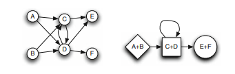
The nodes in a network may be grouped into equivalence classes according to the role they play. Two basic concepts have been developed to formalize the assignments of roles individuals play in social networks: structural and regular equivalence. Both are illustrated in Fig. 2.1. Two nodes are called structurally equivalent if they have the exact same neighbors [12]. This means that in the adjacency matrix of the network, the rows and columns of the corresponding nodes are exactly equal. The idea behind this type of equivalence is that two nodes which have the exact same interaction partners can only perform the exact same function in the network. In Fig. 2.1, only nodes $A$ and $B$ are structurally equivalent while all other nodes are structurally equivalent only to themselves.

To relax this very strict criterion, regular equivalence was introduced [13, 14]. Two nodes are regularly equivalent if they are connected in the same way to equivalent others. Clearly, all nodes which are structurally equivalent must also be regularly equivalent, but not vice versa. The seemingly circular definition of regular equivalence is most easily understood in the following way: Every class of regularly equivalent nodes is represented by a single node in an “image graph”. The nodes in the image graph are connected (disconnected), if connections between nodes in the respective classes exist (are absent) in the original network. In Fig. $2.1$, nodes $A$ and $B, C$ and $D$ as well as $E$ and $F$ form three classes of regular equivalence. If the network in Fig. $2.1$ represents the trade interactions on a market, we may interpret these three classes as producers, retailers and consumers, respectively. Producers sell to retailers, while retailers may sell to other retailers and consumers, which in turn only buy from retailers. The image graph (also “block” or “role model”) hence gives a bird’s-eye view of the network by concentrating on the roles, i.e., the functions, only. Note that no two nodes in the image graph may be structurally equivalent, otherwise the image graph is redundant.

统计代写|复杂网络代写complex networks代考|Block Modeling

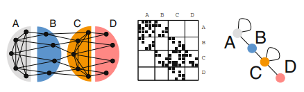
Let us consider the larger example from Fig. 2.2. The network consists of 18 nodes in 4 designed roles. Nodes of type A connect to other nodes of type $A$ and to nodes of type $B$. Those of type $B$ connect to nodes of type $A$ and $C$, Fig. 2.2. An example network and two possible block models. The nodes in this network can be grouped into four classes of regular equivalence ( $A, B, C$ and D). Ordering the rows and columns of the adjacency matrix according to the four classes of regular equivalence makes a block structure apparent (there are 16 blocks from the 4 classes), which is efficiently represented by an image graph.

acting as a kind of intermediary. Nodes of type C have connections to nodes of type $B$, others of type $C$ and of type $D$. Finally, nodes of type $D$ form a kind of periphery to nodes of type C. An ordering of rows and columns according to the types of nodes makes a block structure in the adjacency matrix apparent. Hence the name “block model”. The image graph effectively represents the 4 roles present in the original network and the 16 blocks in the adjacency matrix. Every edge present in the network is represented by an edge in the image graph and all edges absent in the image graph are also absent in the original network.

Regular equivalence, though a looser concept than structural equivalence, is still very strict as it requires the nodes to play their roles exactly, i.e., each node must have at least one of the connections required and may not have any connection forbidden by the role model. In Fig. 2.2, a link between two nodes of type A may be removed without changing the image graph, but an additional link from a node of type $A$ to a node of type $C$ would change the role model completely. Clearly, this is unsatisfactory in situations where the data are noisy or only approximate role models are desired for a very large data set.

复杂网络代写

统计代写|复杂网络代写complex networks代考|Patterns of Link Structure

上述讨论表明了研究现实世界网络中链接结构的重要性。人们可以将此问题视为一种模式检测。模式通常被视为某种规律性的表达。然而，这种规律性可能是什么，通常仍然是一个模糊的概念。将所有内容定义为非随机的规则可能是明智的。
本专着所关注的结构是复杂网络中一种特殊类型的非随机结构，与上述相关性密切相关。关于相关性的部分已经表明，如果网络中不同类型的节点是已知的，则网络的链接结构可能会显示特定的签名。然而，在大多数情况下，不同类型节点的存在只是假设，每个节点的类型是未知的。这项工作的目的是开发方法来检测网络中不同类型节点的存在并找到每个节点的推定类型。来自各个领域的许多可能的应用将再次激发这个问题。

假设我们有一个企业的通信网络。节点是雇员，链接表示它们之间的通信，例如通过电子邮件。然后，我们可能会寻找“实践社区”——彼此之间联系特别紧密的员工，即具有高度丰富的群体内交流。然后可以将这些实践社区与企业的组织结构进行比较，并可能将结果用于未来项目的团队组装。Tyler 等人已经在这个方向进行了研究。[26]。

来自生物学的新实验技术允许自动提取生物体产生的所有蛋白质。蛋白质是生物功能的核心组成部分，但通常，蛋白质不会单独发挥作用，而是相互结合形成复合物，这些复合物又能够执行特定功能，例如启动特定 DNA 片段的转录。现在可以以自动化的方式研究大量蛋白质的成对结合相互作用[27]. 这种研究的结果是一个蛋白质相互作用网络，其中的链接代表蛋白质之间的成对相互作用。蛋白质功能应该反映在这样的网络中。例如，构成复合物一部分的蛋白质现在应该可以作为此类网络中密集互连的节点组进行检测 [28]。分析蛋白质相互作用或其他生物网络的结构

因此，由自动化实验创建是规划未来实验的第一步 [29]。

科学文章的集合代表了一个高度分散的科学知识库[30,31]. 在线数据库使得以自动方式研究这些成为可能，例如以共同作者网络或引文网络的形式。在前者中，节点是研究人员，而链接代表一篇或多篇文章的共同作者。对该网络结构的分析可能会提供有关不同科学家之间合作的宝贵信息，并有助于评估资助政策或影响未来的资助决策。在后者中，网络中的节点是科学文章，链接表示对另一个的引用。分析这个网络的结构可能会深入了解特定科学领域的不同研究领域。

统计代写|复杂网络代写complex networks代考|Positions, Roles and Equivalences

通过调查来自包括生命科学、生态学、信息和社会科学以及经济学在内的广泛来源的数据，研究人员表明，网络拓扑与该网络中节点的功能之间确实存在密切关系[ 1-9]。一个中心思想是具有相似连接模式的节点将执行相似的功能。了解网络的拓扑结构将是了解单个节点功能以及最终了解任何网络动态的第一步。

和以前一样，我们可以将我们的分析建立在社会科学领域所做的工作上。在社交网络的背景下，连接模式与网络中代理的功能相关的想法被称为扮演“角色”或假设“位置”[10,11]. 在这里，我们将赞同这个想法。

网络中的节点可以根据它们所扮演的角色分为等价类。已经开发了两个基本概念来正式确定个人在社会网络中所扮演角色的分配：结构对等和常规对等。两者都如图 2.1 所示。如果两个节点具有完全相同的邻居，则称它们为结构等效的 [12]。这意味着在网络的邻接矩阵中，对应节点的行和列是完全相等的。这种等效性背后的想法是，具有完全相同交互伙伴的两个节点只能在网络中执行完全相同的功能。在图 2.1 中，只有节点一种和乙在结构上等价，而所有其他节点仅在结构上与其自身等价。

为了放宽这个非常严格的标准，引入了正则等价[13, 14]。如果两个节点以相同的方式连接到等价的其他节点，则它们通常是等价的。显然，所有结构等价的节点也必须定期等价，但反之则不然。正则等价看似循环的定义最容易理解为：每类正则等价节点都由“图像图”中的单个节点表示。如果原始网络中各个类中的节点之间存在（不存在）连接，则图像图中的节点是连接的（断开的）。在图。2.1, 节点一种和乙,C和D也和和F形成三类正则等价。如果网络如图2.1代表市场上的贸易互动，我们可以将这三类分别解释为生产者、零售商和消费者。生产者向零售商销售产品，而零售商可能向其他零售商和消费者销售产品，而消费者又只从零售商那里购买。因此，图像图（也称为“块”或“角色模型”）通过仅关注角色（即功能）来提供网络的鸟瞰图。请注意，图像图中没有两个节点在结构上可能是等效的，否则图像图是冗余的。

统计代写|复杂网络代写complex networks代考|Block Modeling

让我们考虑图 2.2 中更大的例子。该网络由 4 个设计角色的 18 个节点组成。类型 A 的节点连接到其他类型的节点一种和类型的节点乙. 那些类型乙连接到类型的节点一种和C，图 2.2。一个示例网络和两个可能的块模型。该网络中的节点可以分为四类正则等价（一种,乙,C和 D)。根据四类正则等价对邻接矩阵的行和列进行排序，使得块结构明显（4 类中有 16 个块），它可以通过图像图有效地表示。

作为一种中介。类型 C 的节点与类型的节点有连接乙, 其他类型C和类型D. 最后，节点类型D对类型 C 的节点形成一种外围。根据节点类型对行和列的排序使得邻接矩阵中的块结构变得明显。因此得名“块模型”。图像图有效地表示了原始网络中存在的 4 个角色和邻接矩阵中的 16 个块。网络中存在的每条边都由图像图中的一条边表示，并且图像图中不存在的所有边在原始网络中也不存在。

正则等价虽然是一个比结构等价更宽松的概念，但仍然非常严格，因为它要求节点准确地发挥自己的作用，即每个节点必须至少有一个所需的连接，并且不能有任何角色模型禁止的连接. 在图 2.2 中，可以在不改变图像图的情况下删除两个 A 类型节点之间的链接，但是可以从类型 A 的节点中删除一个附加链接一种到类型的节点C将彻底改变榜样。显然，这在数据嘈杂或对于非常大的数据集只需要近似角色模型的情况下是不能令人满意的。

统计代写请认准statistics-lab™. statistics-lab™为您的留学生涯保驾护航。统计代写|python代写代考

随机过程代考

在概率论概念中，随机过程是随机变量的集合。 若一随机系统的样本点是随机函数，则称此函数为样本函数，这一随机系统全部样本函数的集合是一个随机过程。 实际应用中，样本函数的一般定义在时间域或者空间域。 随机过程的实例如股票和汇率的波动、语音信号、视频信号、体温的变化，随机运动如布朗运动、随机徘徊等等。

贝叶斯方法代考

贝叶斯统计概念及数据分析表示使用概率陈述回答有关未知参数的研究问题以及统计范式。后验分布包括关于参数的先验分布，和基于观测数据提供关于参数的信息似然模型。根据选择的先验分布和似然模型，后验分布可以解析或近似，例如，马尔科夫链蒙特卡罗 (MCMC) 方法之一。贝叶斯统计概念及数据分析使用后验分布来形成模型参数的各种摘要，包括点估计，如后验平均值、中位数、百分位数和称为可信区间的区间估计。此外，所有关于模型参数的统计检验都可以表示为基于估计后验分布的概率报表。

广义线性模型代考

广义线性模型（GLM）归属统计学领域，是一种应用灵活的线性回归模型。该模型允许因变量的偏差分布有除了正态分布之外的其它分布。

statistics-lab作为专业的留学生服务机构，多年来已为美国、英国、加拿大、澳洲等留学热门地的学生提供专业的学术服务，包括但不限于Essay代写，Assignment代写，Dissertation代写，Report代写，小组作业代写，Proposal代写，Paper代写，Presentation代写，计算机作业代写，论文修改和润色，网课代做，exam代考等等。写作范围涵盖高中，本科，研究生等海外留学全阶段，辐射金融，经济学，会计学，审计学，管理学等全球99%专业科目。写作团队既有专业英语母语作者，也有海外名校硕博留学生，每位写作老师都拥有过硬的语言能力，专业的学科背景和学术写作经验。我们承诺100%原创，100%专业，100%准时，100%满意。

机器学习代写

随着AI的大潮到来，Machine Learning逐渐成为一个新的学习热点。同时与传统CS相比，Machine Learning在其他领域也有着广泛的应用，因此这门学科成为不仅折磨CS专业同学的“小恶魔”，也是折磨生物、化学、统计等其他学科留学生的“大魔王”。学习Machine learning的一大绊脚石在于使用语言众多，跨学科范围广，所以学习起来尤其困难。但是不管你在学习Machine Learning时遇到任何难题，StudyGate专业导师团队都能为你轻松解决。

多元统计分析代考

基础数据: $N$ 个样本， $P$ 个变量数的单样本，组成的横列的数据表
变量定性: 分类和顺序；变量定量：数值
数学公式的角度分为: 因变量与自变量

时间序列分析代写

随机过程，是依赖于参数的一组随机变量的全体，参数通常是时间。 随机变量是随机现象的数量表现，其时间序列是一组按照时间发生先后顺序进行排列的数据点序列。通常一组时间序列的时间间隔为一恒定值（如1秒，5分钟，12小时，7天，1年），因此时间序列可以作为离散时间数据进行分析处理。研究时间序列数据的意义在于现实中，往往需要研究某个事物其随时间发展变化的规律。这就需要通过研究该事物过去发展的历史记录，以得到其自身发展的规律。

回归分析代写

多元回归分析渐进（Multiple Regression Analysis Asymptotics）属于计量经济学领域，主要是一种数学上的统计分析方法，可以分析复杂情况下各影响因素的数学关系，在自然科学、社会和经济学等多个领域内应用广泛。

MATLAB代写

MATLAB 是一种用于技术计算的高性能语言。它将计算、可视化和编程集成在一个易于使用的环境中，其中问题和解决方案以熟悉的数学符号表示。典型用途包括：数学和计算算法开发建模、仿真和原型制作数据分析、探索和可视化科学和工程图形应用程序开发，包括图形用户界面构建MATLAB 是一个交互式系统，其基本数据元素是一个不需要维度的数组。这使您可以解决许多技术计算问题，尤其是那些具有矩阵和向量公式的问题，而只需用 C 或 Fortran 等标量非交互式语言编写程序所需的时间的一小部分。MATLAB 名称代表矩阵实验室。MATLAB 最初的编写目的是提供对由 LINPACK 和 EISPACK 项目开发的矩阵软件的轻松访问，这两个项目共同代表了矩阵计算软件的最新技术。MATLAB 经过多年的发展，得到了许多用户的投入。在大学环境中，它是数学、工程和科学入门和高级课程的标准教学工具。在工业领域，MATLAB 是高效研究、开发和分析的首选工具。MATLAB 具有一系列称为工具箱的特定于应用程序的解决方案。对于大多数 MATLAB 用户来说非常重要，工具箱允许您学习和应用专业技术。工具箱是 MATLAB 函数（M 文件）的综合集合，可扩展 MATLAB 环境以解决特定类别的问题。可用工具箱的领域包括信号处理、控制系统、神经网络、模糊逻辑、小波、仿真等。

R语言代写	问卷设计与分析代写
PYTHON代写	回归分析与线性模型代写
MATLAB代写	方差分析与试验设计代写
STATA代写	机器学习/统计学习代写
SPSS代写	计量经济学代写
EVIEWS代写	时间序列分析代写
EXCEL代写	深度学习代写
SQL代写	各种数据建模与可视化代写

如果你也在 怎样代写复杂网络complex networks这个学科遇到相关的难题，请随时右上角联系我们的24/7代写客服。

复杂网络是由数量巨大的节点和节点之间错综复杂的关系共同构成的网络结构。

statistics-lab™ 为您的留学生涯保驾护航 在代写复杂网络complex networks方面已经树立了自己的口碑, 保证靠谱, 高质且原创的统计Statistics代写服务。我们的专家在代写复杂网络complex networks方面经验极为丰富，各种代写复杂网络complex networks相关的作业也就用不着说。

我们提供的复杂网络complex networks及其相关学科的代写，服务范围广, 其中包括但不限于:

• Statistical Inference 统计推断
• Statistical Computing 统计计算
• Advanced Probability Theory 高等楖率论
• Advanced Mathematical Statistics 高等数理统计学
• (Generalized) Linear Models 广义线性模型
• Statistical Machine Learning 统计机器学习
• Longitudinal Data Analysis 纵向数据分析
• Foundations of Data Science 数据科学基础

统计代写|复杂网络代写complex networks代考|Scale-Free Degree Distributions

With the increasing use of the Internet as a source of information and means of communication as well as the increasing availability of large online databases and repositories, more and more differences between real world networks and random graphs were discovered. Most strikingly was certainly the observation that many real world networks have a degree distribution far from Poissonian with heavy tails which rather follows a log-normal distribution or alternatively a power law.

For networks with a power-law degree distribution the notion of a “scalefree” degree distribution is often used. A scale-free degree distribution is characterized by a power law of the form
$$
P(k) \propto k^{-\gamma}
$$
with some positive exponent $\gamma$. The probability of having $k$ neighbors is inversely proportional to $k^{\gamma}$. The name “scale free” comes from the fact that there is no characteristic value of $k$. While in ER graphs, the characteristic $k$ is the average degree $\langle k\rangle$, i.e., the average is also a typical $k$, there is no typical degree in scale-free networks.

From these observations, it became clear that the assumption of equal linking probability for all pairs of nodes had to be dropped and that specific mechanisms had to be sought which could explain the link pattern of complex networks from a set of rules. Until now, many such models have been introduced which model networks to an almost arbitrary degree of detail. The starting point for this development was most likely the model by Barabási and Albert [16]. They realized that for many real world networks, two key ingredients are crucial: growth and preferential attachment, i.e., nodes that already have a large number of links are more likely to acquire new ones during the growth of the network. These two simple assumptions lead them to develop a network model which produces a scale-free degree distribution of exponent $\gamma=3$. Consequently, this model was used as a first attempt to explain the link distribution of web pages.

In order to model an ensemble of random graphs with a given degree distribution without resorting to some growth model of how the graph is knit the “configuration model” can be used. It is generally attributed to Molloy and Reed [17], who devised an algorithm for constructing actual networks, but it was first introduced by Bender and Canfield [18]. The configuration model assumes a given degree distribution $P(k)$. Every node $i$ is assigned a number of stubs $k_{i}$ according to its degree drawn from $P(k)$ and then the stubs are connected randomly. For this model, the probability that two randomly chosen nodes are connected by an edge can be well approximated by $p_{i j}=k_{i} k_{j} / 2 M$ as long as the degrees of the nodes are smaller than $\sqrt{2 M}$. The probability to find a link between two nodes is hence proportional to the product of the degrees of these two nodes. The configuration model and the ER model make fundamentally different assumptions on the nature of the objects represented by the nodes. In the ER model, fluctuations in the number of connections of a node arise entirely due to chance. In the configuration model, they represent a quality of the node which may be interpreted as some sort of “activity” of the object represented by the node.

统计代写|复杂网络代写complex networks代考|Correlations in Networks

Thus far, only models in which all nodes were equivalent have been introduced. In many networks, however, nodes of different types coexist and the probability of linking between them may depend on the types of nodes. A typical example may be the age of the nodes in a social network. Agents of the same age generally have a higher tendency to interact than agents of different ages. Let us assume the type of each node is already known. One can then ask whether the assumption holds, that links between nodes in the same class are indeed more frequent than links between nodes in different classes. Newman [19] defines the following quantities: $e_{r s}$ as the fraction of edges that fall between nodes in class $r$ and $s$. Further, he defines $\sum_{r} e_{r s}=a_{s}$ as the fraction of edges that are connected to at least one node in class $s$. Note that

$e_{r s}$ can also be interpreted as the probability that a randomly chosen edge lies between nodes of class $r$ and $s$ and that $a_{s}$ can be interpreted as the probability that a randomly chosen edge has at least one end in class $s$. Hence, $a_{s}^{2}$ is the expected fraction of edges connecting two nodes of class $s$. Comparing this expectation value with the true value $e_{s s}$ for all groups $s$ leads to the definition of the “assortativity coefficient” $r_{A}$ :
$$
r_{A}=\frac{\sum_{s}\left(e_{s s}-a_{s}^{2}\right)}{1-\sum_{s} a_{s}^{2}} .
$$
This assortativity coefficient $r_{A}$ is one, if all links fall exclusively between nodes of the same type. Then the network is perfectly “assortative”, but the different classes of nodes remain disconnected. It is zero if $e_{s s}=a_{s}^{2}$ for all classes $s$, i.e., no preference in linkage for either the same or a different class is present. It takes negative values, if edges lie preferably between nodes of different classes, in which case the network is called “disassortative”. The denominator corresponds to a perfectly assortative network. Hence, $r_{A}$ can be interpreted as the percentage to which the network is perfectly assortative.
For the classes of the nodes, any measurable quantity may be used [20]. Especially interesting are investigations into assortative mixing by degree, i.e., do nodes predominantly connect to other nodes of similar degree (assortative, $r_{A}>0$ ) or is the opposite the case (disassortative, $r_{A}<0$ ). It was found that many social networks are assortative, while technological or biological networks are generally disassortative $[20]$. Note that $r_{A}$ may also be generalized to the case where the class index $s$ takes continuous values [20]. It should be stressed that such correlation structures do not affect the degree distribution.

统计代写|复杂网络代写complex networks代考|Dynamics on Networks

Apart from these topological models mainly concerned with link structure, a large number of researchers are concerned with dynamical processes taking place on networks and the influence the network structure has on them. Among the most widely studied processes is epidemic spreading and one of the most salient results is certainly that by Cohen $[21,22]$, which shows that for scale-free topologies with exponents larger than two and low clustering, the epidemic threshold (the infectiousness a pathogen needs to infect a significant portion of the network) drops to zero. The reason for this is, in principle, the fact that for scale-free degree distributions with exponents between 2 and 3 the average number of second neighbors $\langle d\rangle$ may diverge. Liljeros showed that networks of sexual contacts do have indeed such a topology [23]. At the same time, these results brought about suggestions for new vaccination techniques such as the vaccination of acquaintances of randomly selected people which allows us to vaccinate people with higher numbers of connections with higher efficiency [24]. Consequently, a number of researchers are also studying the interplay between topology of the network and dynamic processes on networks

in models that allow dynamic rewiring of connections in accordance with, for instance, games being played on the network to gain insights into the origin of cooperation [25].

All of this research has shown the profound effect of the topology of the connections underlying a dynamical process and hence underlines the importance of thoroughly studying the topology of complex networks.

复杂网络代写

统计代写|复杂网络代写complex networks代考|Scale-Free Degree Distributions

随着互联网作为信息和通信手段的使用越来越多，以及大型在线数据库和存储库的可用性越来越高，现实世界网络和随机图之间的差异越来越大。最引人注目的当然是观察到，许多现实世界的网络的度数分布远离具有重尾的 Poissonian 分布，而是遵循对数正态分布或幂律。

对于具有幂律度分布的网络，经常使用“无标度”度分布的概念。无标度度分布的特征是幂律形式为
磷(ķ)∝ķ−C
有一些正指数C. 拥有的概率ķ邻居成反比ķC. “无标度”的名称来自于没有特征值的事实ķ. 而在 ER 图中，特征ķ是平均学位⟨ķ⟩，即平均值也是一个典型的ķ，无标度网络中没有典型度数。

从这些观察中可以清楚地看出，必须放弃所有节点对的链接概率相等的假设，并且必须寻找可以从一组规则中解释复杂网络的链接模式的特定机制。到目前为止，已经引入了许多这样的模型，它们对网络进行了几乎任意程度的详细建模。这一发展的起点很可能是 Barabási 和 Albert [16] 的模型。他们意识到，对于许多现实世界的网络来说，两个关键因素至关重要：增长和优先连接，即已经拥有大量链接的节点更有可能在网络增长期间获得新的链接。这两个简单的假设导致他们开发了一个网络模型，该模型产生指数的无标度度分布C=3. 因此，该模型被用作解释网页链接分布的第一次尝试。

为了对具有给定度分布的随机图的集合进行建模，而无需求助于图如何编织的一些增长模型，可以使用“配置模型”。它通常归功于 Molloy 和 Reed [17]，他们设计了一种用于构建实际网络的算法，但它首先由 Bender 和 Canfield [18] 引入。配置模型假设给定度数分布磷(ķ). 每个节点一世分配了一些存根ķ一世根据其程度从磷(ķ)然后随机连接存根。对于这个模型，两个随机选择的节点被一条边连接的概率可以很好地近似为p一世j=ķ一世ķj/2米只要节点的度数小于2米. 因此，在两个节点之间找到链接的概率与这两个节点的度数的乘积成正比。配置模型和 ER 模型对节点表示的对象的性质做出了根本不同的假设。在 ER 模型中，节点连接数的波动完全是偶然性的。在配置模型中，它们代表了节点的质量，可以解释为节点所代表的对象的某种“活动”。

统计代写|复杂网络代写complex networks代考|Correlations in Networks

到目前为止，仅引入了所有节点都等效的模型。然而，在许多网络中，不同类型的节点共存，它们之间链接的概率可能取决于节点的类型。一个典型的例子可能是社交网络中节点的年龄。同年龄的代理人通常比不同年龄的代理人有更高的互动倾向。让我们假设每个节点的类型是已知的。然后人们可以询问是否存在这样的假设，即同一类中节点之间的链接确实比不同类中节点之间的链接更频繁。Newman [19] 定义了以下量：和rs作为落在类中节点之间的边的分数r和s. 此外，他定义∑r和rs=一种s作为连接到类中至少一个节点的边的分数s. 注意

和rs也可以解释为随机选择的边位于类节点之间的概率r和s然后一种s可以解释为随机选择的边在类中至少有一个端点的概率s. 因此，一种s2是连接两个类节点的边的预期分数s. 将此期望值与真实值进行比较和ss对于所有组s导致“分类系数”的定义r一种 :
r一种=∑s(和ss−一种s2)1−∑s一种s2.
这个分类系数r一种是一，如果所有链接都只落在相同类型的节点之间。然后网络是完全“分类的”，但不同类别的节点保持断开连接。如果是零和ss=一种s2所有班级s，即不存在对相同或不同类的链接偏好。如果边最好位于不同类的节点之间，则它取负值，在这种情况下，网络被称为“不分类”。分母对应于完美分类网络。因此，r一种可以解释为网络完全匹配的百分比。
对于节点的类别，可以使用任何可测量的数量[20]。特别有趣的是按程度对分类混合的研究，即节点是否主要连接到相似程度的其他节点（分类，r一种>0) 或者是相反的情况 (disassortative,r一种<0）。发现许多社交网络是分类的，而技术或生物网络通常是不分类的[20]. 注意r一种也可以推广到类索引的情况s取连续值 [20]。需要强调的是，这种相关结构不会影响度数分布。

统计代写|复杂网络代写complex networks代考|Dynamics on Networks

除了这些主要关注链接结构的拓扑模型外，还有大量研究人员关注网络上发生的动态过程以及网络结构对它们的影响。研究最广泛的过程之一是流行病传播，最显着的结果之一当然是科恩的[21,22]，这表明对于指数大于 2 和低聚类的无标度拓扑，流行阈值（病原体感染大部分网络所需的传染性）降至零。其原因原则上是，对于指数在 2 到 3 之间的无标度度分布，第二个邻居的平均数量⟨d⟩可能会发散。Liljeros 表明，性接触网络确实具有这样的拓扑结构 [23]。同时，这些结果为新的疫苗接种技术带来了建议，例如对随机选择的人的熟人进行疫苗接种，这使我们能够以更高的效率为具有更多联系数的人接种疫苗[24]。因此，许多研究人员也在研究网络拓扑与网络动态过程之间的相互作用。

例如，在允许根据网络上正在玩的游戏动态重新布线连接的模型中，以深入了解合作的起源[25]。

所有这些研究都表明了动态过程背后的连接拓扑的深远影响，因此强调了深入研究复杂网络拓扑的重要性。

统计代写请认准statistics-lab™. statistics-lab™为您的留学生涯保驾护航。统计代写|python代写代考

随机过程代考

在概率论概念中，随机过程是随机变量的集合。 若一随机系统的样本点是随机函数，则称此函数为样本函数，这一随机系统全部样本函数的集合是一个随机过程。 实际应用中，样本函数的一般定义在时间域或者空间域。 随机过程的实例如股票和汇率的波动、语音信号、视频信号、体温的变化，随机运动如布朗运动、随机徘徊等等。

贝叶斯方法代考

贝叶斯统计概念及数据分析表示使用概率陈述回答有关未知参数的研究问题以及统计范式。后验分布包括关于参数的先验分布，和基于观测数据提供关于参数的信息似然模型。根据选择的先验分布和似然模型，后验分布可以解析或近似，例如，马尔科夫链蒙特卡罗 (MCMC) 方法之一。贝叶斯统计概念及数据分析使用后验分布来形成模型参数的各种摘要，包括点估计，如后验平均值、中位数、百分位数和称为可信区间的区间估计。此外，所有关于模型参数的统计检验都可以表示为基于估计后验分布的概率报表。

广义线性模型代考

广义线性模型（GLM）归属统计学领域，是一种应用灵活的线性回归模型。该模型允许因变量的偏差分布有除了正态分布之外的其它分布。

statistics-lab作为专业的留学生服务机构，多年来已为美国、英国、加拿大、澳洲等留学热门地的学生提供专业的学术服务，包括但不限于Essay代写，Assignment代写，Dissertation代写，Report代写，小组作业代写，Proposal代写，Paper代写，Presentation代写，计算机作业代写，论文修改和润色，网课代做，exam代考等等。写作范围涵盖高中，本科，研究生等海外留学全阶段，辐射金融，经济学，会计学，审计学，管理学等全球99%专业科目。写作团队既有专业英语母语作者，也有海外名校硕博留学生，每位写作老师都拥有过硬的语言能力，专业的学科背景和学术写作经验。我们承诺100%原创，100%专业，100%准时，100%满意。

机器学习代写

随着AI的大潮到来，Machine Learning逐渐成为一个新的学习热点。同时与传统CS相比，Machine Learning在其他领域也有着广泛的应用，因此这门学科成为不仅折磨CS专业同学的“小恶魔”，也是折磨生物、化学、统计等其他学科留学生的“大魔王”。学习Machine learning的一大绊脚石在于使用语言众多，跨学科范围广，所以学习起来尤其困难。但是不管你在学习Machine Learning时遇到任何难题，StudyGate专业导师团队都能为你轻松解决。

多元统计分析代考

基础数据: $N$ 个样本， $P$ 个变量数的单样本，组成的横列的数据表
变量定性: 分类和顺序；变量定量：数值
数学公式的角度分为: 因变量与自变量

时间序列分析代写

随机过程，是依赖于参数的一组随机变量的全体，参数通常是时间。 随机变量是随机现象的数量表现，其时间序列是一组按照时间发生先后顺序进行排列的数据点序列。通常一组时间序列的时间间隔为一恒定值（如1秒，5分钟，12小时，7天，1年），因此时间序列可以作为离散时间数据进行分析处理。研究时间序列数据的意义在于现实中，往往需要研究某个事物其随时间发展变化的规律。这就需要通过研究该事物过去发展的历史记录，以得到其自身发展的规律。

回归分析代写

多元回归分析渐进（Multiple Regression Analysis Asymptotics）属于计量经济学领域，主要是一种数学上的统计分析方法，可以分析复杂情况下各影响因素的数学关系，在自然科学、社会和经济学等多个领域内应用广泛。

MATLAB代写

MATLAB 是一种用于技术计算的高性能语言。它将计算、可视化和编程集成在一个易于使用的环境中，其中问题和解决方案以熟悉的数学符号表示。典型用途包括：数学和计算算法开发建模、仿真和原型制作数据分析、探索和可视化科学和工程图形应用程序开发，包括图形用户界面构建MATLAB 是一个交互式系统，其基本数据元素是一个不需要维度的数组。这使您可以解决许多技术计算问题，尤其是那些具有矩阵和向量公式的问题，而只需用 C 或 Fortran 等标量非交互式语言编写程序所需的时间的一小部分。MATLAB 名称代表矩阵实验室。MATLAB 最初的编写目的是提供对由 LINPACK 和 EISPACK 项目开发的矩阵软件的轻松访问，这两个项目共同代表了矩阵计算软件的最新技术。MATLAB 经过多年的发展，得到了许多用户的投入。在大学环境中，它是数学、工程和科学入门和高级课程的标准教学工具。在工业领域，MATLAB 是高效研究、开发和分析的首选工具。MATLAB 具有一系列称为工具箱的特定于应用程序的解决方案。对于大多数 MATLAB 用户来说非常重要，工具箱允许您学习和应用专业技术。工具箱是 MATLAB 函数（M 文件）的综合集合，可扩展 MATLAB 环境以解决特定类别的问题。可用工具箱的领域包括信号处理、控制系统、神经网络、模糊逻辑、小波、仿真等。

R语言代写	问卷设计与分析代写
PYTHON代写	回归分析与线性模型代写
MATLAB代写	方差分析与试验设计代写
STATA代写	机器学习/统计学习代写
SPSS代写	计量经济学代写
EVIEWS代写	时间序列分析代写
EXCEL代写	深度学习代写
SQL代写	各种数据建模与可视化代写

如果你也在 怎样代写复杂网络complex networks这个学科遇到相关的难题，请随时右上角联系我们的24/7代写客服。

复杂网络是由数量巨大的节点和节点之间错综复杂的关系共同构成的网络结构。

statistics-lab™ 为您的留学生涯保驾护航 在代写复杂网络complex networks方面已经树立了自己的口碑, 保证靠谱, 高质且原创的统计Statistics代写服务。我们的专家在代写复杂网络complex networks方面经验极为丰富，各种代写复杂网络complex networks相关的作业也就用不着说。

我们提供的复杂网络complex networks及其相关学科的代写，服务范围广, 其中包括但不限于:

• Statistical Inference 统计推断
• Statistical Computing 统计计算
• Advanced Probability Theory 高等楖率论
• Advanced Mathematical Statistics 高等数理统计学
• (Generalized) Linear Models 广义线性模型
• Statistical Machine Learning 统计机器学习
• Longitudinal Data Analysis 纵向数据分析
• Foundations of Data Science 数据科学基础

统计代写|复杂网络代写complex networks代考|Graph Theoretical Notation

Mathematically, a network is represented as a graph $\mathcal{S}(V, E)$, i.e., an object that consists of a set of nodes or vertices $V$ representing the objects or agents in the network and a set $E$ of edges or links or connections representing the interactions or relations of the nodes. The cardinality of these sets, i.e, the number of nodes and edges, is generally denoted by $N$ and $M$, respectively. One may assign different values $w_{i j}$ to the links between nodes $i$ and $j$ in $E$, rendering an edge weighted or otherwise non-weighted ( $w_{i j}=1$ by convention, if one is only interested in the presence or absence of the relation). The number of connections of node $i$ is denoted by its degree $k_{i}$. One can represent the set of edges conveniently in an $N \times N$ matrix $A_{i j}$, called the adjacency matrix. $A_{i j}=w_{i j}$ if an edge between node $i$ and $j$ is present and zero otherwise. Relations may be directed, in which case $A_{i j}$ is non-symmetric $\left(A_{i j} \neq A_{j i}\right)$ or undirected in which case $A_{i j}$ is symmetric. Here, we are mainly concerned with networks in which self-links are absent $\left(A_{i i}=0, \forall i \in V\right)$. In case of a directed network, $A_{i j}$ denotes an outgoing edge from $i$ to $j$. Hence, the outgoing links of node $i$ are found in row $i$, while the incoming links to $i$ are found in column $i$. For undirected networks, it is clear that $\sum_{j=1}^{N} A_{i j}=k_{i}$. For directed networks, $\sum_{j=1} A_{i j}=k_{i}^{\text {out }}$ is the out-degree and equivalently $\sum_{j=1} A_{j i}=k_{i}^{i n}$ is the in-degree of node $i$. It is understood that in undirected networks, the sum of degrees of all nodes in the network equals twice the number of edges $\sum_{i=1}^{N} k_{i}=2 M$. The distribution of the number of connections per node is called degree distribution $P(k)$ and denotes the probability that a randomly chosen node from the network has degree $k$. The average degree in the network is denoted by $\langle k\rangle$ and one has $N\langle k\rangle=2 M$. One can define a

probability $p=2 M / N(N-1)=\langle k\rangle /(N-1)$ as the probability that an edge exists between two randomly chosen nodes from the network.

An (induced) subgraph is a subset of nodes $v \subseteq V$ with $n$ nodes and edges $e \subseteq E$ connecting only the nodes in $v$. A path is a sequence of nodes, subsequent nodes in the sequence being connected by edges from $E$. A node $i$ is called reachable from node $j$ if there exists a path from $j$ to $i$. A subgraph is said to be connected if every node in the subgraph is reachable from every other. The number of steps (links) in the shortest path between two nodes $i$ and $j$ is called the geodesic distance $d(i, j)$ between nodes $i$ and $j$. A network is generally not connected, but may consist of several connected components. The largest of the shortest path distances between any pair of nodes in a connected component is called the diameter of a connected component. The analysis in this monograph shall be restricted to connected components only since it can be repeated on every single one of the connected components of a network. More details on graph theory may be found in the book by Bollobás $[2]$.

With these notations and terms in mind, let us now turn to a brief overview of some aspects of physicists research on networks.

统计代写|复杂网络代写complex networks代考|Random Graphs

For the study of the topology of the interactions of a complex system it is of central importance to have proper random null models of networks, i.e., models of how a graph arises from a random process. Such models are needed for comparison with real world data. When analyzing the structure of real world networks, the null hypothesis shall always be that the link structure is due to chance alone. This null hypothesis may only be rejected if the link structure found differs significantly from an expectation value obtained from a random model. Any deviation from the random null model must be explained by non-random processes.

The most important model of a random graph is due to Erdös and Rényi (ER) [12]. They consider the following two ensembles of random graphs: $\mathcal{G}(N, M)$ and $\mathcal{G}(N, p)$. The first is the ensemble of all graphs with $N$ nodes and exactly $M$ edges. A graph from this ensemble is created by placing the $M$ edges randomly between the $N(N-1) / 2$ possible pairs of nodes. The second ensemble is that of all graphs in which a link between two arbitrarily chosen nodes is present with probability $p$. The expectation value for the number of links of a graph from this ensemble is $\langle M\rangle=p N(N-1) / 2$. In the limit of $N \rightarrow \infty$, the two ensembles are equivalent with $p=2 M / N(N-1)$. The typical graph from these ensembles has a Poissonian degree distribution
$$
P(k)=e^{-\langle k\rangle} \frac{\langle k\rangle^{k}}{k !} .
$$
Here, $\langle k\rangle=p(N-1)=2 M / N$ denotes the average degree in the network.

The properties of ER random graphs have been studied for considerable time and an overview of results can be found in the book by Bollobás [13]. Note that the equivalence of the two ensembles is a remarkable result. If all networks with a given number of nodes and links are taken to be equally probable, then the typical graph from this ensemble will have a Poissonian degree distribution. To draw a graph with a non-Poissonian degree distribution from this ensemble is highly improbable, unless there is a mechanism which leads to a different degree distribution. This issue will be discussed below in more detail.

Another aspect of random networks is worth mentioning: the average shortest path between any pair of nodes scales only as the logarithm of the system size. This is easily seen: Starting from a randomly chosen node, we can visit $\langle k\rangle$ neighbors with a single step. How many nodes can we explore with the second step? Coming from node $i$ to node $j$ via a link between them, we now have $d_{j}=k_{j}-1$ options to proceed. Since we have $k_{j}$ possible ways to arrive at node $j$, the average number of second step neighbors is hence $\langle d\rangle=\sum_{k=2}^{\infty}(k-1) k P(k) /\left(\sum_{k}^{\infty} k P(k)\right)=\left\langle k^{2}\right\rangle /\langle k\rangle-1$. Hence, after two steps we may explore $\langle k\rangle\langle d\rangle$ nodes and after $m$ steps $\langle k\rangle\langle d\rangle^{m-1}$ nodes which means that the entire network may be explored in $m \approx \log N$ steps. This also shows that even in very large random networks, all nodes may be reached with relatively few steps. The number $d=k-1$ of possible ways to exit from a node after entering it via one of its links is also called the “excess degree” of a node. Its distribution $q(d)=(d+1) P(d+1) /\langle k\rangle$ is called the “excess degree distribution” and plays a central role in the analysis of many dynamical phenomena on networks. Note that our estimate is based on the assumption that in every new step we explore $\langle d\rangle$ nodes which we have not seen before! For ER networks, though, this is a reasonable assumption. However, consider a regular lattice as a counterexample. There, the average shortest distance between any pair of nodes scales linearly with the size of the lattice.

统计代写|复杂网络代写complex networks代考|Six Degrees of Separation

The question of short distances was one of the first addressed in the study of real world networks by Stanley Milgram [14]. It was known among sociologists that social networks are characterized by a high local clustering coefficient:
$$
c_{i}=\frac{2 m_{i}}{k_{i}\left(k_{i}-1\right)}
$$
Here, $m_{i}$ is the number of connections among the $k_{i}$ neighbors of node $i$. In other words, $c_{i}$ measures the probability of the neighbors of node $i$ being connected, that is, the probability that the friends of node $i$ are friends among each other. The average of this clustering coefficient over the set of nodes in the network is much higher in social networks than for ER random networks with the same number of nodes and links where $\langle c\rangle=p$. This would mean that the average shortest distance between randomly chosen nodes in social networks may not scale logarithmically with the system size. To test this, Milgram performed the following experiment: He gave out letters in Omaha, Nebraska, and asked the initial recipients of the letters to give the letters only to acquaintances whom they would address by their first name and require that those would do the same when passing the letter on. The letters were addressed to a stock broker living in Boston and unknown to the initial recipients of the letter. Surprisingly, not only did a large number of letters arrive at the destination, but the median of the number of steps it took was only 6. This means the path lengths in social networks may be surprisingly short despite the high local clustering. Even more surprisingly, the agents in this network are able to efficiently navigate messages through the entire network even though they only know the local topology. After this discovery, Duncan Watts and Steve Strogatz [15] provided the first model of a network that combines the high clustering characteristic for acquaintance networks and the short average path lengths known from ER random graphs. At the same time, it retains the fact that there is only a finite number of connections or friends per node in the network. The Watts/Strogatz model came to be known as the “small world model” for complex networks. It basically consists of a regular structure producing a high local clustering and a number of randomly interwoven shortcuts responsible for the short average path length. It was found analytically that a small number of shortcuts, added randomly, suffice to change the scaling of the average shortest path length from linear with system size to logarithmically with system size.

复杂网络代写

统计代写|复杂网络代写complex networks代考|Graph Theoretical Notation

在数学上，网络表示为图小号(在,和)，即由一组节点或顶点组成的对象在表示网络中的对象或代理和一个集合和表示节点的交互或关系的边或链接或连接。这些集合的基数，即节点和边的数量，通常表示为ñ和米， 分别。可以分配不同的值在一世j到节点之间的链接一世和j在和，渲染边缘加权或其他非加权（在一世j=1按照惯例，如果一个人只对关系的存在或不存在感兴趣）。节点的连接数一世用它的度数表示ķ一世. 可以方便地表示一组边ñ×ñ矩阵一种一世j，称为邻接矩阵。一种一世j=在一世j如果节点之间有一条边一世和j存在，否则为零。关系可以被定向，在这种情况下一种一世j是非对称的(一种一世j≠一种j一世)或在这种情况下是无向的一种一世j是对称的。在这里，我们主要关注没有自链接的网络(一种一世一世=0,∀一世∈在). 在有向网络的情况下，一种一世j表示从一世到j. 因此，节点的传出链接一世在行中找到一世，而传入的链接到一世在列中找到一世. 对于无向网络，很明显∑j=1ñ一种一世j=ķ一世. 对于有向网络，∑j=1一种一世j=ķ一世出去 是出度，等价∑j=1一种j一世=ķ一世一世n是节点的入度一世. 可以理解的是，在无向网络中，网络中所有节点的度数之和等于边数的两倍∑一世=1ñķ一世=2米. 每个节点的连接数分布称为度数分布磷(ķ)表示从网络中随机选择的节点具有度数的概率ķ. 网络中的平均度数表示为⟨ķ⟩一个有ñ⟨ķ⟩=2米. 可以定义一个

可能性p=2米/ñ(ñ−1)=⟨ķ⟩/(ñ−1)作为从网络中随机选择的两个节点之间存在边的概率。

（诱导）子图是节点的子集在⊆在和n节点和边和⊆和只连接节点在. 路径是一系列节点，序列中的后续节点由来自的边连接和. 一个节点一世被称为从节点可达j如果存在从j到一世. 如果子图中的每个节点都可以相互访问，则称该子图是连通的。两个节点之间最短路径的步数（链接）一世和j称为测地线距离d(一世,j)节点之间一世和j. 一个网络通常没有连接，但可能由几个连接的组件组成。连通分量中任意一对节点之间的最短路径距离中的最大值称为连通分量的直径。本专着中的分析应仅限于连接组件，因为它可以在网络的每个连接组件上重复。关于图论的更多细节可以在 Bollobás 的书中找到[2].

考虑到这些符号和术语，现在让我们简要概述一下物理学家对网络的研究的某些方面。

统计代写|复杂网络代写complex networks代考|Random Graphs

对于复杂系统相互作用的拓扑结构的研究，具有适当的网络随机零模型（即图如何从随机过程产生的模型）至关重要。需要这样的模型来与现实世界的数据进行比较。在分析现实世界网络的结构时，零假设应始终是链接结构仅由偶然性引起。仅当发现的链接结构与从随机模型获得的期望值显着不同时，才能拒绝该零假设。任何与随机零模型的偏差都必须用非随机过程来解释。

随机图最重要的模型归功于 Erdös 和 Rényi (ER) [12]。他们考虑以下两个随机图集合：G(ñ,米)和G(ñ,p). 第一个是所有图的集合ñ节点和准确米边缘。通过放置米边缘之间随机ñ(ñ−1)/2可能的节点对。第二个集合是所有图的集合，其中两个任意选择的节点之间的链接以概率存在p. 来自该集成的图的链接数的期望值为⟨米⟩=pñ(ñ−1)/2. 在限度内ñ→∞, 这两个集合等价于p=2米/ñ(ñ−1). 这些集合的典型图具有泊松度分布
磷(ķ)=和−⟨ķ⟩⟨ķ⟩ķķ!.
这里，⟨ķ⟩=p(ñ−1)=2米/ñ表示网络中的平均度数。

ER 随机图的性质已经研究了相当长的时间，结果概述可以在 Bollobás [13] 的书中找到。请注意，这两个集合的等价性是一个显着的结果。如果具有给定数量的节点和链接的所有网络都被认为是等概率的，那么来自该集成的典型图将具有泊松度分布。从这个集合中绘制具有非泊松度分布的图是非常不可能的，除非有一种机制导致不同的度分布。这个问题将在下面更详细地讨论。

随机网络的另一个方面值得一提：任何一对节点之间的平均最短路径仅与系统大小的对数成比例。这很容易看出：从一个随机选择的节点开始，我们可以访问⟨ķ⟩一步到位的邻居。第二步可以探索多少个节点？来自节点一世到节点j通过它们之间的链接，我们现在有了dj=ķj−1选项继续。既然我们有ķj到达节点的可能方式j，因此第二步邻居的平均数为⟨d⟩=∑ķ=2∞(ķ−1)ķ磷(ķ)/(∑ķ∞ķ磷(ķ))=⟨ķ2⟩/⟨ķ⟩−1. 因此，经过两个步骤，我们可以探索⟨ķ⟩⟨d⟩节点及之后米脚步⟨ķ⟩⟨d⟩米−1节点，这意味着可以探索整个网络米≈日志⁡ñ脚步。这也表明，即使在非常大的随机网络中，也可以通过相对较少的步骤到达所有节点。数字d=ķ−1通过其中一个链接进入节点后退出节点的可能方式也称为节点的“过度度”。它的分布q(d)=(d+1)磷(d+1)/⟨ķ⟩被称为“过度度分布”，在分析网络上的许多动态现象中起着核心作用。请注意，我们的估计是基于这样一个假设，即在我们探索的每一个新步骤中⟨d⟩我们从未见过的节点！然而，对于 ER 网络，这是一个合理的假设。然而，考虑一个正则格作为反例。在那里，任何一对节点之间的平均最短距离与格子的大小成线性关系。

统计代写|复杂网络代写complex networks代考|Six Degrees of Separation

短距离问题是 Stanley Milgram [14] 在现实世界网络研究中首先解决的问题之一。社会学家知道，社交网络的特点是局部聚集系数很高：
C一世=2米一世ķ一世(ķ一世−1)
这里，米一世是之间的连接数ķ一世节点的邻居一世. 换句话说，C一世测量节点邻居的概率一世被连接，即节点的朋友的概率一世是彼此之间的朋友。在社交网络中，网络中节点集上的聚类系数的平均值远高于具有相同节点和链接数量的 ER 随机网络，其中⟨C⟩=p. 这意味着社交网络中随机选择的节点之间的平均最短距离可能不会与系统大小成对数关系。为了验证这一点，米尔格拉姆进行了以下实验：他在内布拉斯加州的奥马哈寄出信件，并要求最初的收信人只将信件给他们会直呼其名的熟人，并要求他们也这样做在传递这封信时。这些信件是寄给住在波士顿的一位股票经纪人的，最初的收件人不知道。令人惊讶的是，不仅有大量信件到达目的地，而且所走步数的中位数也只有 6 步。这意味着社交网络中的路径长度可能会非常短，尽管局部聚类程度很高。更令人惊讶的是，该网络中的代理能够有效地在整个网络中导航消息，即使它们只知道本地拓扑。在这一发现之后，Duncan Watts 和 Steve Strogatz [15] 提供了第一个网络模型，该模型结合了熟人网络的高聚类特性和从 ER 随机图中已知的短平均路径长度。同时，它保留了网络中每个节点只有有限数量的连接或朋友的事实。Watts/Strogatz 模型被称为复杂网络的“小世界模型”。它基本上由一个产生高局部聚类的规则结构和许多随机交织的捷径组成，这些捷径负责较短的平均路径长度。分析发现，少量的快捷方式，随机添加，

统计代写请认准statistics-lab™. statistics-lab™为您的留学生涯保驾护航。统计代写|python代写代考

随机过程代考

在概率论概念中，随机过程是随机变量的集合。 若一随机系统的样本点是随机函数，则称此函数为样本函数，这一随机系统全部样本函数的集合是一个随机过程。 实际应用中，样本函数的一般定义在时间域或者空间域。 随机过程的实例如股票和汇率的波动、语音信号、视频信号、体温的变化，随机运动如布朗运动、随机徘徊等等。

贝叶斯方法代考

贝叶斯统计概念及数据分析表示使用概率陈述回答有关未知参数的研究问题以及统计范式。后验分布包括关于参数的先验分布，和基于观测数据提供关于参数的信息似然模型。根据选择的先验分布和似然模型，后验分布可以解析或近似，例如，马尔科夫链蒙特卡罗 (MCMC) 方法之一。贝叶斯统计概念及数据分析使用后验分布来形成模型参数的各种摘要，包括点估计，如后验平均值、中位数、百分位数和称为可信区间的区间估计。此外，所有关于模型参数的统计检验都可以表示为基于估计后验分布的概率报表。

广义线性模型代考

广义线性模型（GLM）归属统计学领域，是一种应用灵活的线性回归模型。该模型允许因变量的偏差分布有除了正态分布之外的其它分布。

statistics-lab作为专业的留学生服务机构，多年来已为美国、英国、加拿大、澳洲等留学热门地的学生提供专业的学术服务，包括但不限于Essay代写，Assignment代写，Dissertation代写，Report代写，小组作业代写，Proposal代写，Paper代写，Presentation代写，计算机作业代写，论文修改和润色，网课代做，exam代考等等。写作范围涵盖高中，本科，研究生等海外留学全阶段，辐射金融，经济学，会计学，审计学，管理学等全球99%专业科目。写作团队既有专业英语母语作者，也有海外名校硕博留学生，每位写作老师都拥有过硬的语言能力，专业的学科背景和学术写作经验。我们承诺100%原创，100%专业，100%准时，100%满意。

机器学习代写

随着AI的大潮到来，Machine Learning逐渐成为一个新的学习热点。同时与传统CS相比，Machine Learning在其他领域也有着广泛的应用，因此这门学科成为不仅折磨CS专业同学的“小恶魔”，也是折磨生物、化学、统计等其他学科留学生的“大魔王”。学习Machine learning的一大绊脚石在于使用语言众多，跨学科范围广，所以学习起来尤其困难。但是不管你在学习Machine Learning时遇到任何难题，StudyGate专业导师团队都能为你轻松解决。

多元统计分析代考

基础数据: $N$ 个样本， $P$ 个变量数的单样本，组成的横列的数据表
变量定性: 分类和顺序；变量定量：数值
数学公式的角度分为: 因变量与自变量

时间序列分析代写

随机过程，是依赖于参数的一组随机变量的全体，参数通常是时间。 随机变量是随机现象的数量表现，其时间序列是一组按照时间发生先后顺序进行排列的数据点序列。通常一组时间序列的时间间隔为一恒定值（如1秒，5分钟，12小时，7天，1年），因此时间序列可以作为离散时间数据进行分析处理。研究时间序列数据的意义在于现实中，往往需要研究某个事物其随时间发展变化的规律。这就需要通过研究该事物过去发展的历史记录，以得到其自身发展的规律。

回归分析代写

多元回归分析渐进（Multiple Regression Analysis Asymptotics）属于计量经济学领域，主要是一种数学上的统计分析方法，可以分析复杂情况下各影响因素的数学关系，在自然科学、社会和经济学等多个领域内应用广泛。

MATLAB代写

MATLAB 是一种用于技术计算的高性能语言。它将计算、可视化和编程集成在一个易于使用的环境中，其中问题和解决方案以熟悉的数学符号表示。典型用途包括：数学和计算算法开发建模、仿真和原型制作数据分析、探索和可视化科学和工程图形应用程序开发，包括图形用户界面构建MATLAB 是一个交互式系统，其基本数据元素是一个不需要维度的数组。这使您可以解决许多技术计算问题，尤其是那些具有矩阵和向量公式的问题，而只需用 C 或 Fortran 等标量非交互式语言编写程序所需的时间的一小部分。MATLAB 名称代表矩阵实验室。MATLAB 最初的编写目的是提供对由 LINPACK 和 EISPACK 项目开发的矩阵软件的轻松访问，这两个项目共同代表了矩阵计算软件的最新技术。MATLAB 经过多年的发展，得到了许多用户的投入。在大学环境中，它是数学、工程和科学入门和高级课程的标准教学工具。在工业领域，MATLAB 是高效研究、开发和分析的首选工具。MATLAB 具有一系列称为工具箱的特定于应用程序的解决方案。对于大多数 MATLAB 用户来说非常重要，工具箱允许您学习和应用专业技术。工具箱是 MATLAB 函数（M 文件）的综合集合，可扩展 MATLAB 环境以解决特定类别的问题。可用工具箱的领域包括信号处理、控制系统、神经网络、模糊逻辑、小波、仿真等。

R语言代写	问卷设计与分析代写
PYTHON代写	回归分析与线性模型代写
MATLAB代写	方差分析与试验设计代写
STATA代写	机器学习/统计学习代写
SPSS代写	计量经济学代写
EVIEWS代写	时间序列分析代写
EXCEL代写	深度学习代写
SQL代写	各种数据建模与可视化代写