
如果你也在 怎样代写神经网络neural networks这个学科遇到相关的难题,请随时右上角联系我们的24/7代写客服。
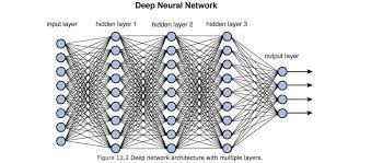
神经网络,也被称为人工神经网络(ANN)或模拟神经网络(SNN),是机器学习的一个子集,是深度学习算法的核心。它们的名称和结构受到人脑的启发,模仿了生物神经元相互之间的信号方式。
statistics-lab™ 为您的留学生涯保驾护航 在代写神经网络neural networks方面已经树立了自己的口碑, 保证靠谱, 高质且原创的统计Statistics代写服务。我们的专家在代写神经网络neural networks代写方面经验极为丰富,各种代写神经网络neural networks相关的作业也就用不着说。
计算机代写|神经网络代写neural networks代考|C alculating th e N o d e D eltas
The first step is to calculate a constant value for every node, or neuron, in the neural network. We will start with the output nodes and work our way backwards through the neural network – this is where the term, backpropagation, comes from. We initially calculate the errors for the output neurons and propagate these errors backwards through the neural network.
The value that we will calculate for each node is called the node delta. The term, layer delta, is also sometimes used to describe this value. Layer delta describes the fact that these deltas are calculated one layer at a time. The method for calculating the node deltas differs depending on whether you are calculating for an output or interior node. The output neurons are, obviously, all output nodes. The hidden and input neurons are the interior nodes. The equation to calculate the node delta is provided in Equation 4.1.
Equation 4.1: Calculating the Node Deltas
$$
\delta_i= \begin{cases}-E f_i^{\prime}, & , \text { output nodes } \ f_i^{\prime} \sum_k \omega_{h i} \delta_k & , \text { interier nodes }\end{cases}
$$
We will calculate the node delta for all hidden and non-bias neurons. There is no need to calculate the node delta for the input and bias neurons. Even though the node delta can easily be calculated for input and bias neurons using the above equation, these values are not needed for the gradient calculation. As you will soon see, gradient calculation for a weight only looks at the neuron that the weight is connected to. Bias and input neurons are only the beginning point for a connection. They are never the end point.
We will begin by using the formula for the output neurons. You will notice that the formula uses a value $\mathbf{E}$. This is the error for this output neuron. You can see how to calculate $\mathbf{E}$ from Equation 4.2.
Equation 4.2: The Error Function
$$
E=(a-i)
$$
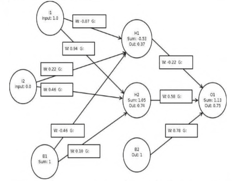
You may recall a similar equation to Equation 2.1 from Chapter 2. This is the error function. Here, we subtract the ideal from the actual. For the neural network provided in Figure 4.2, this can be written like this:
$$
E=0.75-1.00=-0.25
$$
Now that we have $\mathbf{E}$, we can calculate the node delta for the first (and only) output node. Filling in Equation 4.1, we get the following:
$$
-(-0.25) * d A(1.1254)=0.185 * 0.25=0.05
$$
计算机代写|神经网络代写neural networks代考|C alculating the Individual Gradients
We can now calculate the individual gradients. Unlike the node deltas, only one equation is used to calculate the actual gradient. A gradient is calculated using Equation 4.5.
Equation 4.5: Individual Gradient
$$
\frac{\partial E}{\partial w_{(i k)}}=\delta_k \cdot o_j
$$
The above equation calculates the partial derivative of the error (E) with respect to each individual weight. The partial derivatives are the gradients. Partial derivatives were discussed in Chapter 3. To determine an individual gradient, multiply the node delta for the target neuron by the weight from the source neuron. In the above equation, $\mathbf{k}$ represents the target neuron and $\mathbf{i}$ represents the source neuron.
To calculate the gradient for the weight from $\mathbf{H 1}$ to $\mathbf{O 1}$, the following values would be used:
$$
\begin{aligned}
& \text { output }(\mathrm{h} 1) * \text { nodeDe1ta (o1) } \
& (0.37 * 0.05)=0.01677
\end{aligned}
$$
It is important to note that in the above equation, we are multiplying by the output of hidden 1 , not the sum. When dealing directly with a derivative you should supply the sum. Otherwise, you would be indirectly applying the activation function twice. In the above equation, we are not dealing directly with the derivative, so we use the regular node output. The node output has already had the activation function applied.
Once the gradients are calculated, the individual positions of the weights no longer matter. We can simply think of the weights and gradients as single dimensional arrays. The individual training methods that we will look at will treat all weights and gradients equally. It does not matter if a weight is from an input neuron or an output neuron. It is only important that the correct weight is used with the correct gradient. The ordering of these weight and gradient arrays is arbitrary. However, Encog uses the following order for the above neural network:
Weight/Gradient 0 : Hidden $1 \rightarrow$ Output 1
Weight/Gradient 1 : Hidden $2 \rightarrow$ Output 1
Weight/Gradient 2 : Bias $2 \rightarrow$ Output 1
Weight/Gradient 3 : Input $1 \rightarrow$ Hidden 1
Weight/Gradient 4 : Input $2 \rightarrow$ Hidden 1
Weight/Gradient 5 : Bias $1->$ Hidden 1
Weight/Gradient 6 : Input $1->$ Hidden 2
Weight/Gradient 7 : Input $2 \rightarrow$ Hidden 2
Weight/Gradient $8:$ Bias $1 \rightarrow$ Hidden 2
Weight/Gradient D: Hidden 1 -> Output 1
Weight/Gradient 1: Hidden 2 -> Output 1
Weight/Gradient 2: Bias $2 \rightarrow$ Output 1
Weight/Gradient 3 : Input $1 \rightarrow$ Hidden 1
Weight/Gradient 4 : Input $2 \rightarrow$ Hidden 1
Weight/Gradient 5: Bias 1 Hidden 1
Weight/Gradient 6: Input $1->$ Hidden 2
Weight/Gradient 7: Input $2 \rightarrow$ Hidden 2
Weight/Gradient 8: Bias $1 \rightarrow$ Hidden 2
神经网络代写
计算机代写|神经网络代写neural networks代考|C alculating th e N o d e D eltas
第一步是为神经网络中的每个节点或神经元计算一个恒定值。我们将从输出节点开始,通过神经网络往回走——这就是反向传播这个术语的由来。我们首先计算输出神经元的误差,并通过神经网络向后传播这些误差。
我们将为每个节点计算的值称为节点增量。术语“层增量”有时也用来描述这个值。层增量描述了这些增量一次计算一层的事实。计算节点增量的方法取决于计算的是输出节点还是内部节点。输出神经元显然是所有的输出节点。隐藏神经元和输入神经元是内部节点。节点delta的计算公式如式4.1所示。
式4.1:计算节点delta
$ $
\delta_i= \begin{cases}-E f_i^{\prime}, &, \text{输出节点}\ f_i^{\prime} \sum_k \omega_{h i} \delta_k &, \text{中间节点}\end{cases}
$ $
我们将计算所有隐藏和无偏差神经元的节点delta。不需要计算输入和偏置神经元的节点delta。尽管使用上述方程可以很容易地计算输入和偏倚神经元的节点delta,但梯度计算不需要这些值。你很快就会看到,权重的梯度计算只关注与该权重相连的神经元。偏差和输入神经元只是连接的起点。它们永远不是终点。
我们将从使用输出神经元的公式开始。您将注意到公式使用了一个值$\mathbf{E}$。这是输出神经元的误差。您可以从公式4.2中看到如何计算$\mathbf{E}$。
式4.2:误差函数
$ $
E =(ⅰ)
$ $
你可能还记得第2章中类似的方程2.1。这是误差函数。这里,我们用实际减去理想。对于图4.2所提供的神经网络,可以这样写:
$ $
E = 0.75 – -1.00 = -0.25
$ $
现在我们有了$\mathbf{E}$,我们可以计算第一个(也是唯一一个)输出节点的节点增量。代入式4.1,可得:
$ $
-(-0.25) * d A(1.1254)=0.185 * 0.25=0.05
$ $
计算机代写|神经网络代写neural networks代考|C alculating the Individual Gradients
现在我们可以计算单个梯度了。与节点delta不同,只使用一个方程来计算实际的梯度。梯度由式4.5计算。
方程4.5:个体梯度
$ $
\压裂{\部分E}{\部分w_ {(k)}} = \ delta_k \ cdot o_j
$ $
上面的方程计算误差(E)相对于每个单独的权重的偏导数。偏导数是梯度。第三章讨论偏导数。为了确定单个梯度,将目标神经元的节点增量乘以源神经元的权重。在上式中,$\mathbf{k}$表示目标神经元,$\mathbf{i}$表示源神经元。
要计算从$\mathbf{H 1}$到$\mathbf{O 1}$的权重梯度,将使用以下值:
$ $
开始{对齐}
& \text {output}(\ mathm {h} 1) * \text {nodeDe1ta (o1)} \
& (0.37 * 0.05)=0.01677
结束{对齐}
$ $
重要的是要注意,在上面的等式中,我们乘以隐藏1的输出,而不是总和。当直接处理导数时,应该给出和。否则,您将间接地应用激活函数两次。在上面的方程中,我们没有直接处理导数,所以我们使用常规的节点输出。节点输出已经应用了激活函数。
一旦计算出梯度,权重的单个位置就不再重要了。我们可以简单地把权重和梯度看作是单维数组。我们将看到的个别训练方法将平等地对待所有权重和梯度。权重是来自输入神经元还是输出神经元并不重要。重要的是,正确的权重与正确的梯度一起使用。这些权重和梯度数组的顺序是任意的。然而,Encog对上述神经网络使用以下顺序:
权重/梯度0:隐藏$1 \右箭头$输出1
权重/梯度1:隐藏$2 \右箭头$输出1
权重/梯度2:偏置$2 \右移$输出1
权重/梯度3:输入$1 \右箭头$隐藏1
权重/梯度4:输入$2 \右箭头$隐藏1
权重/梯度5:偏差$1->$隐藏1
权重/梯度6:输入$1->$ Hidden 2
权重/梯度7:输入$2 \右箭头$隐藏2
权重/梯度$8:$ Bias $1 \右箭头$隐藏2
权重/梯度D:隐藏1 ->输出1
权重/梯度1:隐藏2 ->输出1
权重/梯度2:偏置$2 \右移$输出1
权重/梯度3:输入$1 \右箭头

统计代写请认准statistics-lab™. statistics-lab™为您的留学生涯保驾护航。
金融工程代写
金融工程是使用数学技术来解决金融问题。金融工程使用计算机科学、统计学、经济学和应用数学领域的工具和知识来解决当前的金融问题,以及设计新的和创新的金融产品。
非参数统计代写
非参数统计指的是一种统计方法,其中不假设数据来自于由少数参数决定的规定模型;这种模型的例子包括正态分布模型和线性回归模型。
广义线性模型代考
广义线性模型(GLM)归属统计学领域,是一种应用灵活的线性回归模型。该模型允许因变量的偏差分布有除了正态分布之外的其它分布。
术语 广义线性模型(GLM)通常是指给定连续和/或分类预测因素的连续响应变量的常规线性回归模型。它包括多元线性回归,以及方差分析和方差分析(仅含固定效应)。
有限元方法代写
有限元方法(FEM)是一种流行的方法,用于数值解决工程和数学建模中出现的微分方程。典型的问题领域包括结构分析、传热、流体流动、质量运输和电磁势等传统领域。
有限元是一种通用的数值方法,用于解决两个或三个空间变量的偏微分方程(即一些边界值问题)。为了解决一个问题,有限元将一个大系统细分为更小、更简单的部分,称为有限元。这是通过在空间维度上的特定空间离散化来实现的,它是通过构建对象的网格来实现的:用于求解的数值域,它有有限数量的点。边界值问题的有限元方法表述最终导致一个代数方程组。该方法在域上对未知函数进行逼近。[1] 然后将模拟这些有限元的简单方程组合成一个更大的方程系统,以模拟整个问题。然后,有限元通过变化微积分使相关的误差函数最小化来逼近一个解决方案。
tatistics-lab作为专业的留学生服务机构,多年来已为美国、英国、加拿大、澳洲等留学热门地的学生提供专业的学术服务,包括但不限于Essay代写,Assignment代写,Dissertation代写,Report代写,小组作业代写,Proposal代写,Paper代写,Presentation代写,计算机作业代写,论文修改和润色,网课代做,exam代考等等。写作范围涵盖高中,本科,研究生等海外留学全阶段,辐射金融,经济学,会计学,审计学,管理学等全球99%专业科目。写作团队既有专业英语母语作者,也有海外名校硕博留学生,每位写作老师都拥有过硬的语言能力,专业的学科背景和学术写作经验。我们承诺100%原创,100%专业,100%准时,100%满意。
随机分析代写
随机微积分是数学的一个分支,对随机过程进行操作。它允许为随机过程的积分定义一个关于随机过程的一致的积分理论。这个领域是由日本数学家伊藤清在第二次世界大战期间创建并开始的。
时间序列分析代写
随机过程,是依赖于参数的一组随机变量的全体,参数通常是时间。 随机变量是随机现象的数量表现,其时间序列是一组按照时间发生先后顺序进行排列的数据点序列。通常一组时间序列的时间间隔为一恒定值(如1秒,5分钟,12小时,7天,1年),因此时间序列可以作为离散时间数据进行分析处理。研究时间序列数据的意义在于现实中,往往需要研究某个事物其随时间发展变化的规律。这就需要通过研究该事物过去发展的历史记录,以得到其自身发展的规律。
回归分析代写
多元回归分析渐进(Multiple Regression Analysis Asymptotics)属于计量经济学领域,主要是一种数学上的统计分析方法,可以分析复杂情况下各影响因素的数学关系,在自然科学、社会和经济学等多个领域内应用广泛。
MATLAB代写
MATLAB 是一种用于技术计算的高性能语言。它将计算、可视化和编程集成在一个易于使用的环境中,其中问题和解决方案以熟悉的数学符号表示。典型用途包括:数学和计算算法开发建模、仿真和原型制作数据分析、探索和可视化科学和工程图形应用程序开发,包括图形用户界面构建MATLAB 是一个交互式系统,其基本数据元素是一个不需要维度的数组。这使您可以解决许多技术计算问题,尤其是那些具有矩阵和向量公式的问题,而只需用 C 或 Fortran 等标量非交互式语言编写程序所需的时间的一小部分。MATLAB 名称代表矩阵实验室。MATLAB 最初的编写目的是提供对由 LINPACK 和 EISPACK 项目开发的矩阵软件的轻松访问,这两个项目共同代表了矩阵计算软件的最新技术。MATLAB 经过多年的发展,得到了许多用户的投入。在大学环境中,它是数学、工程和科学入门和高级课程的标准教学工具。在工业领域,MATLAB 是高效研究、开发和分析的首选工具。MATLAB 具有一系列称为工具箱的特定于应用程序的解决方案。对于大多数 MATLAB 用户来说非常重要,工具箱允许您学习和应用专业技术。工具箱是 MATLAB 函数(M 文件)的综合集合,可扩展 MATLAB 环境以解决特定类别的问题。可用工具箱的领域包括信号处理、控制系统、神经网络、模糊逻辑、小波、仿真等。