如果你也在 怎样代写数值分析numerical analysis这个学科遇到相关的难题,请随时右上角联系我们的24/7代写客服。
数值分析是数学的一个分支,使用数字近似法解决连续问题。它涉及到设计能给出近似但精确的数字解决方案的方法,这在精确解决方案不可能或计算成本过高的情况下很有用。
statistics-lab™ 为您的留学生涯保驾护航 在代写数值分析numerical analysis方面已经树立了自己的口碑, 保证靠谱, 高质且原创的统计Statistics代写服务。我们的专家在代写数值分析numerical analysis代写方面经验极为丰富,各种代写数值分析numerical analysis相关的作业也就用不着说。
我们提供的数值分析numerical analysis及其相关学科的代写,服务范围广, 其中包括但不限于:
- Statistical Inference 统计推断
- Statistical Computing 统计计算
- Advanced Probability Theory 高等概率论
- Advanced Mathematical Statistics 高等数理统计学
- (Generalized) Linear Models 广义线性模型
- Statistical Machine Learning 统计机器学习
- Longitudinal Data Analysis 纵向数据分析
- Foundations of Data Science 数据科学基础
数学代写|数值分析代写numerical analysis代考|Constructing interpolants in the Lagrange basis
The monomial basis gave us a linear system (1.1) of the form Ac $=\mathbf{f}$ in which A was a dense matrix: all of its entries are nonzero. The Newton basis gave a simpler system (1.4) in which A was a lower triangular matrix. Can we go one step further, and find a set of basis functions for which the matrix in (1.3) is diagonal?
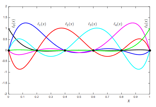
For the matrix to be diagonal, the $j$ th basis function would need to have roots at all the other interpolation points $x_k$ for $k \neq j$. Such func-tions, denoted $\ell_j$ for $j=0, \ldots, n$, are called Lagrange basis polynomials, and they result in the Lagrange form of the interpolating polynomial.
We seek to construct $\ell_j \in \mathcal{P}_n$ with $\ell_j\left(x_k\right)=0$ if $j \neq k$, but $\ell_j\left(x_k\right)=1$ if $j=k$. That is, $\ell_j$ takes the value one at $x_j$ and has roots at all the other $n$ interpolation points.
What form do these basis functions $\ell_j \in \mathcal{P}n$ take? Since $\ell_j$ is a degree- $n$ polynomial with the $n$ roots $\left{x_k\right}{k=0, k \neq j^{\prime}}^n$ it can be written in the form
$$
\ell_j(x)=\prod_{k=0, k \neq j}^n \gamma_k\left(x-x_k\right)
$$
for appropriate constants $\gamma_k$. We can force $\ell_j\left(x_j\right)=1$ if all the terms in the above product are one when $x=x_j$, i.e., when $\gamma_k=1 /\left(x_j-\right.$ $\left.x_k\right)$, so that
$$
\ell_j(x)=\prod_{k=0, k \neq j}^n \frac{x-x_k}{x_j-x_k} .
$$
This form makes it clear that $\ell_j\left(x_j\right)=1$. With these new basis functions, the constants $\left{c_j\right}$ can be written down immediately. The interpolating polynomial has the form
$$
p_n(x)=\sum_{k=0}^n c_k \ell_k(x)
$$
数学代写|数值分析代写numerical analysis代考|Convergence theory for polynomial interpolation
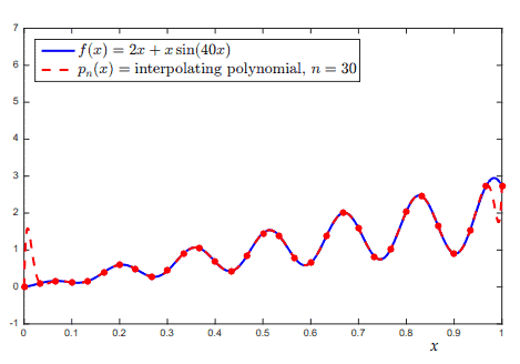
Interpolation can be used to generate low-degree polynomials that approximate a complicated function over the interval $[a, b]$. One might assume that the more data points that are interpolated (for a fixed $[a, b]$ ), the more accurate the resulting approximation. In this lecture, we address the behavior of the maximum error
$$
\max _{x \in[a, b]}\left|f(x)-p_n(x)\right|
$$
as the number of interpolation points-hence, the degree of the interpolating polynomial-is increased. We begin with a theoretical result.
Unfortunately, we do not have time to prove this in class. ${ }^{\text {As }}$ stated, this theorem gives no hint about what the approximating polynomial looks like, whether $p_n$ interpolates $f$ at $n+1$ points, or merely approximates $f$ well throughout $[a, b]$, nor does the Weierstrass theorem describe the accuracy of a polynomial for a specific value of $n$ (though one could gain insight into such questions by studying the constructive proof).
On the other hand, for the interpolation problem studied in the preceding lectures, we can obtain a specific error formula that gives a bound on $\max {x \in[a, b]}\left|f(x)-p_n(x)\right|$. From this bound, we can deduce if interpolating $f$ at increasingly many points will eventually yield a polynomial approximation to $f$ that is accurate to any specified precision. For any $\hat{x} \in[a, b]$ that is not of the interpolation points, we seek to measure the error $$ f(\widehat{x})-p_n(\widehat{x}), $$ where $p_n \in \mathcal{P}_n$ is the interpolant to $f$ at the distinct points $x_0, \ldots, x_n \in$ $[a, b]$. We can get a grip on this error from the following perspective. Extend $p_n$ by one degree to give a new polynomial that additionally interpolates $f$ at $\widehat{x}$. This is easy to do with the Newton form of the interpolant; write the new polynomial as $$ p_n(x)+\lambda \prod{j=0}^n\left(x-x_j\right)
$$ for constant $\lambda$ chosen so that
$$
f(\widehat{x})=p_n(\widehat{x})+\lambda \prod_{j=0}^n\left(\widehat{x}-x_j\right)
$$
数值分析代考
数学代写|数值分析代写numerical analysis代考|Constructing interpolants in the Lagrange basis
单项式基础为我们提供了 $A C$ 形式的线性系统 (1.1)= f其中 $A$ 是一个密集矩阵: 它的所有条目都是非零的。牛 顿基础给出了一个更简单的系统 (1.4),其中 $\mathrm{A}$ 是下三角矩阵。我们能不能更进一步,找到一组基函数,使得 (1.3) 中的矩阵是对角线的?
对于对角矩阵, $j$ th 基函数需要在所有其他揷值点都有根 $x_k$ 为了 $k \neq j$. 这样的功能,记为 $\ell_j$ 为了 $j=0, \ldots, n$ ,被称为拉格朗日基多项式,它们导致揷值多项式的拉格朗日形式。
我们寻求构建 $\ell_j \in \mathcal{P}n$ 和 $\ell_j\left(x_k\right)=0$ 如果 $j \neq k$ ,但 $\ell_j\left(x_k\right)=1$ 如果 $j=k$. 那是, $\ell_j$ 取值一 $x_j$ 并在所有其 他地方扎根 $n$ 揷值点。 这些基函数的形式是什么 $\ell_j \in \mathcal{P} n$ 拿? 自从 $\ell_j$ 是学位 $n$ 多项式与 $n$ 根 $\backslash$ \eft ${\mathrm{x}$ $\backslash \backslash$ right $}\left{\mathrm{k}=0, \mathrm{k} \backslash \ln \mathrm{j}^{\wedge}{\backslash \mathrm{prime}}\right}^{\wedge} \mathrm{n}$ 它可以写成这样
$$
\ell_j(x)=\prod_{k=0, k \neq j}^n \gamma_k\left(x-x_k\right)
$$
对于适当的常数 $\gamma_k$. 我们可以强制 $\ell_j\left(x_j\right)=1$ 如果上述产品中的所有条款都是一个时 $x=x_j$ ,即,当 $\gamma_k=1 /\left(x_j-x_k\right)$ ,以便
$$
\ell_j(x)=\prod_{k=0, k \neq j}^n \frac{x-x_k}{x_j-x_k}
$$
这个表格清楚地表明 $\ell_j\left(x_j\right)=1$. 有了这些新的基函数,常数 $\backslash$ 左 ${\mathrm{c}$ j右 $}$ 可以立即写下来。揷值多项式具有以下 形式
$$
p_n(x)=\sum_{k=0}^n c_k \ell_k(x)
$$
数学代写|数值分析代写numerical analysis代考|Convergence theory for polynomial interpolation
揷值可用于生成在区间内逼近复杂函数的低次多项式 $[a, b]$. 人们可能会假设揷值的数据点越多 (对于固定的 $[a, b]$ ),得到的近似值越准确。在本讲中,我们将讨论最大误差的行为
$$
\max {x \in[a, b]}\left|f(x)-p_n(x)\right| $$ 随着揷值点的数量一一因此,揷值多项式的次数一一增加。我们从一个理论结果开始。 不幸的是,我们没有时间在课堂上证明这一点。As 声明,这个定理没有给出近似多项式的暗示,无论是 $p_n$ 内揷 $f$ 在 $n+1$ 点,或仅仅是近似值 $f$ 贯穿始终 $[a, b]$ , Weierstrass 定理也没有描述特定值的多项式的精度 $n$ (尽管可 以通过研究建设性证据来深入了解伩些问题)。 另一方面,对于前几讲研究的揷值问题,我们可以得到一个特定的误差公式,它给出了一个边界 $\max x \in[a, b]\left|f(x)-p_n(x)\right|$. 从这个界限,我们可以推断出如果揷值 $f$ 在越来越多的点最终会产生多项式 近似 $f$ 准确到任何指定的精度。对于任何 $\hat{x} \in[a, b]$ 那不是揷值点,我们试图测量误差 $$ f(\widehat{x})-p_n(\widehat{x}), $$ 在哪里 $p_n \in \mathcal{P}_n$ 是揷值到 $f$ 在不同的点 $x_0, \ldots, x_n \in[a, b]$. 我们可以从以下角度来把握这个错误。延长 $p_n$ 增 加一个度数以给出一个新的多项式,该多项式另外揷值 $f$ 在 $\widehat{x}$. 使用揷值的牛顿形式很容易做到这一点; 将新多项 式写为 $$ p_n(x)+\lambda \prod j=0^n\left(x-x_j\right) $$ 对于常量 $\lambda$ 选择这样 $$ f(\widehat{x})=p_n(\widehat{x})+\lambda \prod{j=0}^n\left(\widehat{x}-x_j\right)
$$

统计代写请认准statistics-lab™. statistics-lab™为您的留学生涯保驾护航。
金融工程代写
金融工程是使用数学技术来解决金融问题。金融工程使用计算机科学、统计学、经济学和应用数学领域的工具和知识来解决当前的金融问题,以及设计新的和创新的金融产品。
非参数统计代写
非参数统计指的是一种统计方法,其中不假设数据来自于由少数参数决定的规定模型;这种模型的例子包括正态分布模型和线性回归模型。
广义线性模型代考
广义线性模型(GLM)归属统计学领域,是一种应用灵活的线性回归模型。该模型允许因变量的偏差分布有除了正态分布之外的其它分布。
术语 广义线性模型(GLM)通常是指给定连续和/或分类预测因素的连续响应变量的常规线性回归模型。它包括多元线性回归,以及方差分析和方差分析(仅含固定效应)。
有限元方法代写
有限元方法(FEM)是一种流行的方法,用于数值解决工程和数学建模中出现的微分方程。典型的问题领域包括结构分析、传热、流体流动、质量运输和电磁势等传统领域。
有限元是一种通用的数值方法,用于解决两个或三个空间变量的偏微分方程(即一些边界值问题)。为了解决一个问题,有限元将一个大系统细分为更小、更简单的部分,称为有限元。这是通过在空间维度上的特定空间离散化来实现的,它是通过构建对象的网格来实现的:用于求解的数值域,它有有限数量的点。边界值问题的有限元方法表述最终导致一个代数方程组。该方法在域上对未知函数进行逼近。[1] 然后将模拟这些有限元的简单方程组合成一个更大的方程系统,以模拟整个问题。然后,有限元通过变化微积分使相关的误差函数最小化来逼近一个解决方案。
tatistics-lab作为专业的留学生服务机构,多年来已为美国、英国、加拿大、澳洲等留学热门地的学生提供专业的学术服务,包括但不限于Essay代写,Assignment代写,Dissertation代写,Report代写,小组作业代写,Proposal代写,Paper代写,Presentation代写,计算机作业代写,论文修改和润色,网课代做,exam代考等等。写作范围涵盖高中,本科,研究生等海外留学全阶段,辐射金融,经济学,会计学,审计学,管理学等全球99%专业科目。写作团队既有专业英语母语作者,也有海外名校硕博留学生,每位写作老师都拥有过硬的语言能力,专业的学科背景和学术写作经验。我们承诺100%原创,100%专业,100%准时,100%满意。
随机分析代写
随机微积分是数学的一个分支,对随机过程进行操作。它允许为随机过程的积分定义一个关于随机过程的一致的积分理论。这个领域是由日本数学家伊藤清在第二次世界大战期间创建并开始的。
时间序列分析代写
随机过程,是依赖于参数的一组随机变量的全体,参数通常是时间。 随机变量是随机现象的数量表现,其时间序列是一组按照时间发生先后顺序进行排列的数据点序列。通常一组时间序列的时间间隔为一恒定值(如1秒,5分钟,12小时,7天,1年),因此时间序列可以作为离散时间数据进行分析处理。研究时间序列数据的意义在于现实中,往往需要研究某个事物其随时间发展变化的规律。这就需要通过研究该事物过去发展的历史记录,以得到其自身发展的规律。
回归分析代写
多元回归分析渐进(Multiple Regression Analysis Asymptotics)属于计量经济学领域,主要是一种数学上的统计分析方法,可以分析复杂情况下各影响因素的数学关系,在自然科学、社会和经济学等多个领域内应用广泛。
MATLAB代写
MATLAB 是一种用于技术计算的高性能语言。它将计算、可视化和编程集成在一个易于使用的环境中,其中问题和解决方案以熟悉的数学符号表示。典型用途包括:数学和计算算法开发建模、仿真和原型制作数据分析、探索和可视化科学和工程图形应用程序开发,包括图形用户界面构建MATLAB 是一个交互式系统,其基本数据元素是一个不需要维度的数组。这使您可以解决许多技术计算问题,尤其是那些具有矩阵和向量公式的问题,而只需用 C 或 Fortran 等标量非交互式语言编写程序所需的时间的一小部分。MATLAB 名称代表矩阵实验室。MATLAB 最初的编写目的是提供对由 LINPACK 和 EISPACK 项目开发的矩阵软件的轻松访问,这两个项目共同代表了矩阵计算软件的最新技术。MATLAB 经过多年的发展,得到了许多用户的投入。在大学环境中,它是数学、工程和科学入门和高级课程的标准教学工具。在工业领域,MATLAB 是高效研究、开发和分析的首选工具。MATLAB 具有一系列称为工具箱的特定于应用程序的解决方案。对于大多数 MATLAB 用户来说非常重要,工具箱允许您学习和应用专业技术。工具箱是 MATLAB 函数(M 文件)的综合集合,可扩展 MATLAB 环境以解决特定类别的问题。可用工具箱的领域包括信号处理、控制系统、神经网络、模糊逻辑、小波、仿真等。